Abstract
A better understanding of mixing times for mixed solvent systems in laboratory-scale vessels is crucial for improving mixing-sensitive processes such as antisolvent crystallisation. Whilst mixing in agitated vessels has been extensively studied using solutions of additives in the same solvent, there is very limited literature on the mixing of different miscible solvents and none which would be relevant to antisolvent crystallisation processes. In this work, the mixing times of water–ethanol systems in a 1 litre vessel, agitated by a pitched blade impeller with probes used as baffles, were investigated in the transitional flow regime using both experimental and computational fluid dynamics (CFD) approaches. We studied two scenarios: adding sodium chloride tracer to premixed water–ethanol solutions and adding ethanol containing a tracer to water. Mixing was investigated experimentally through conductivity measurements and computationally using large eddy simulations with the M-Star CFD software package. Empirical correlations from the Dynochem engineering toolbox were also used for comparison. The results showed significant run-to-run variability in the mixing times from both experiments and CFD simulations, with experimental ranges being notably wider than CFD ones under the given conditions. While the CFD simulations showed consistent mixing times across different solvent compositions, the experimental mixing times decreased with increasing ethanol content. The mixing times were approximately inversely proportional to the impeller speed. The CFD simulations indicated that 25–40 impeller rotations were required for homogenisation, while the experiments needed 25–100 rotations. The Dynochem correlations predicted 40 rotations, independent of speed, but could not capture the inherent variability of the mixing times.
1. Introduction
In chemical and pharmaceutical manufacturing, heat and mass transfer significantly influence the performance of the manufacturing process steps, such as synthesis or crystallisation. These transport phenomena are influenced by agitation in vessels with mixing conditions varying widely across development stages and process steps; thus, mixing is an important aspect of process design. Crystallisation processes are particularly sensitive to mixing, as temperature or concentration gradients can produce inhomogeneity in the prevailing level of supersaturation. This can result in regions of high supersaturation close to the walls of the vessel in cooling crystallisation or at the addition location for antisolvent or reactive crystallisation processes. This affects crystallisation outcomes and can lead to scaling on vessel walls or inlet ports.
The mixing time is considered as one of the most important factors in assessing the performance of agitated systems. The mixing time can be defined as the time required for achieving a certain degree of homogeneity of tracer inserted in a stirred vessel [1]. Computational fluid dynamics (CFD) can be used to estimate mixing times and provide further insight into how different mixing configurations influence supersaturation gradients within a crystallisation vessel. CFD can be used to develop strategies for the rational scale up of processes involving the mixing of miscible liquids, such as antisolvent crystallisation. However, these models require validation to assess the reliability and accuracy of the predicted outcomes. This can be achieved by comparing the models to the relevant experimental data. Previously, Oblak et al. performed a digital twinning process for stirred tank reactors through tandem experimental and CFD simulations to evaluate mixing in baffled and unbaffled vessels. A single liquid system of distilled water was used [2]. In their work, it was found that the system geometry influenced the mixing time: irregular flow distribution can lead to local stagnation zones, thereby increasing the time needed to achieve the homogenisation of the liquid phase composition. It was also found that measuring local, point-wise concentrations can lead to an underestimation of the global mixing time required for the homogenisation of the entire vessel. In another paper, the mixing times were predicted for miscible solvents using a CFD approach, which was qualitatively compared to experimental work [3]. The characterisation of mixing from the pilot to manufacturing scale using an experimental and CFD hybrid approach was developed by Martinetz et al. [4]. This approach enabled the mixing times to be correlated to the vessel filling volume and vessel-averaged energy dissipation rate for single-phase systems.
There are many experimental techniques that can be used to characterise mixing times in agitated vessels, with varying degrees of accuracy and reproducibility. When categorising mixing characterisation techniques, they can be divided into two groups based on the volume of fluid represented by the measurement [5]. The first of these are local techniques, in which only localised measurement using fixed probes is provided. The mixing times are then estimated based on a set homogenisation criteria, for example, a property such as the conductivity to reach 95% of the fully mixed value. Whilst they are simple to implement, provide direct measurements, and can be used for transparent and opaque fluids, they are intrusive and disturb the measured flow fields. Additionally, the resulting mixing time is dependent on the probe position, and care must be taken in selecting a location that is representative of the mixing times [6,7]. To obtain more spatial information on the process, multiple probes can be used together. Another characterisation technique is the application of planar laser-induced fluorescence (pLIF) combined with image analysis. Here, the measurements are made on the laser plane, and only a limited spatial resolution is provided. Advantages of this technique include the non-intrusiveness with regard to the fluid, as well as the provision of detailed visualisation of the fluid structures and mixing patterns of the systems. The applications of pLIF are limited by the difficulty in calibrating, as well as the high laser power/costs associated with large volumes or opaque fluids [8,9].
Global mixing characterisation methods offer spatial information on the whole vessel, can provide quantitative information on the global flow structures, and highlight regions of poor mixing. One such method is colourimetry, in which colour changes are used to determine mixing times. One example is fast acid–base reactions involving colour changes [5,10]. Further advantages of this method are its non-intrusiveness, simple implementation, and limited calibration requirements [6,11]. The accuracy of this method can be improved when combined with image analysis technique to quantify the colour change process and define individual RBG model criteria to define the end of mixing [5,12]. Liquid crystal thermography can be used to induce colour changes in vessels [6,12,13]. Thermochromic liquid crystals are suspended in the liquid, and the thermal pulse is given. The resulting mixing of this pulse leads to the crystals exhibiting a different colour depending on the local temperature. The temperature profile of the vessel is then determined using the crystal colours and is used as the scalar to characterise the mixing. Image processing is typically used to analyse the results to more accurately quantify the evolution of colour change.
Electrical resistance tomography (ERT) is a non-invasive method based on conductivity that is typically used for solutions that have a distinct conductivity change upon mixing [5,14]. Through capturing a series of 2D tomograms, ERT is capable of proving a visualisation of 3D flow fields, allowing for good spatial and temporal resolution of the system to be obtained. The cost and complexity in setting up ERT is considerable and as such is mainly used for applications in which detailed flow fields are required, for example, for mixing characterisation in concentrated slurries [15] or to determine gas/liquid flow patterns [16], as opposed to characterising the mixing times of vessels.
Whilst optical methods such as colourimetry are relatively simple, they can only be applied to optically transparent vessels and fluids, significantly limiting their industrially relevant geometries [17]. Although tomography can provide detailed information on flow patterns, it has several practical drawbacks when using manufacturing equipment, such as the limited space for sensor installation, waste material treatment, and strict regulations for equipment in a GMP environment [17]. Local mixing characterisation techniques such as probe-based methods are an attractive option due to the relative easiness of application to industrial vessels, i.e., the insertion of the probe being straightforward in most cases. The main disadvantage of using a probe is that only local flow properties are measured, leading to limited spatial and temporal information being provided on the measured quantity. To account for this during measuring mixing time determination, careful consideration must be taken on deciding the placement of the probe. A position should be used that gives a good representation of the global mixing time within the vessel. The probe sensor response time should be fast in comparison to mixing kinetics, and a data measurement frequency of at least once per second is recommended [4]. The mixing times in agitated vessels can be determined using tracer tests, with probes being used to provide information on the measured variable, such as Ph or conductivity. In this work, we use the conductivity method, which involves the addition of a salt tracer and measuring the conductivity increase within the vessel. The mixing time can be determined once the conductivity fluctuations are less than 5% of the homogenised value, referred to as the 95% mixing assumption [18].
Antisolvent crystallisation involves the mixing of miscible liquids with different viscosities and densities, which can influence mixing phenomenology and kinetics in agitated vessels. Bouwmans et al. presented work on the influence of viscosity and density differences on mixing times in stirred vessels [19]. To vary the viscosity and density independently, mixtures of water, ethanol, and glycerol were used in which Poly-Vinyl-Pyrrolidone (PVP) was dissolved to achieve the desired viscosity allowing for systems ranging from 1 mPas to 200 mPas and 900 kg/m3 to 1100 kg/m3, respectively. Under certain conditions, they found that the mixing time can be unpredictable due to the turbulent nature of flow, leading to mixing time standard deviations of over 50%. Their conclusions were based on the case of a less dense liquid being added to the surface of a bulk liquid and can be summarised as follows: relatively short mixing times with a large relative standard deviation were found at high stirrer speeds, whilst longer mixing times with small relative standard deviation were found at low stirrer speeds. In the transitional region, both mechanisms were at work, giving low mixing time predictability and large relative standard deviations.
Whilst mixing in agitated vessels has been extensively studied using solutions of various additives in the same solvent to modify viscosities and densities, for example [19,20,21], there is only very limited CFD simulation literature on the mixing of different miscible solvents [3,22,23], and none of them would be relevant to antisolvent crystallisation processes. We address this gap by investigating the mixing times in water–ethanol systems for the first time using both experimental and computational approaches. We quantify the mixing time variability in the transitional flow regime, which is particularly relevant for lab-scale antisolvent crystallisation. Several techniques for characterising the mixing times are compared, including conductivity measurements, computational tracer concentration tracking, and empirical correlations. The combined use of experimental measurements, CFD simulations, and empirical correlations enables direct comparison of these methods for characterising both mixing times and their intrinsic uncertainties in transitional flow regimes. This approach provides a deeper understanding of the inherent variability of mixing processes, offering practical insights for laboratory-scale mixing processes.
The remainder of this paper will be organised as follows. In the methods section, we describe the experimental methods and CFD. The results and discussion section is divided into three subsections: mixing time characterisation, mixing times in premixed water/ethanol solvent mixtures, and the addition of ethanol to water. The main outcomes of the work are then summarised in the conclusion section.
2. Methods
This section presents the methodology used in this research. It is organised into four distinct components: Section 2.1 describes the experimental setup and procedures; Section 2.2 outlines the computational fluid dynamics (CFD) simulations; Section 2.3 explains the implementation of the empirical software toolbox Dynochem; and Section 2.4 defines the analytical approaches used to characterise mixing times.
2.1. Experimental
In this article, we investigate mixing times of miscible solvent systems in a 1 L stirred vessel. The miscible liquids were selected to represent a common antisolvent pair: water and ethanol. Two distinct cases were considered, one in which the solvents were ‘premixed’ and the other where we investigated the addition of ethanol to water. For the former, water and ethanol were mixed prior to the salt tracer being added, with sufficient time given to ensure a fully homogenised solution. Salt tracer was then injected as a concentrated aqueous solution at the surface of the solvent mixture. In the latter, salt tracer was added to either the solvent or antisolvent before mixing the solvents. Conductivity as a function of time was measured during the mixing process, allowing for mixing times to to be determined. The subsequent section will describe the experimental procedure and setup used in this work.
2.1.1. Mixing Vessel Setup
The Mettler Toledo Optimax 1001 Thermostat System (Columbus, OH, USA) was utilised for all experiments without the use of baffles. The total volume was kept constant at 1 L. A metal downward pitched-blade impeller (Mettler Toledo 103504) with four blades at 45° was used. The impeller had a 45 mm outer diameter and was positioned 19 mm above the bottom of the vessel. Two probes (conductivity and temperature) were placed 38 mm from the bottom of the vessel and positioned at 30° angles. The conductivity probe (Mettler Toledo InPro 7100(i) Series) was connected to an external logger to record measurements every 0.1 s. The temperature probe measured the temperature of the vessel contents. The vessel jacket temperature was also recorded. Figure 1 shows a schematic of the vessel setup.
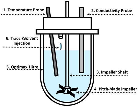
Figure 1.
Schematic of the Mettler Toledo Optimax 1001 system. A metal downward pitched-blade impeller with 4 blades with OD of 45 mm was placed 19 mm above the bottom of the vessel. Two probes (conductivity and temperature) were placed 38 mm from the bottom of the vessel and positioned at 30° angles. Numbers correspond to components in Table 1, where geometries used in the experimental work are summarised.
2.1.2. Tracer Tests
Sodium chloride (NaCl) was dissolved in distilled water to prepare 1 M salt tracer solution. Solvent mixtures used in all experiments comprised of water and ethanol, with relative ratio of water to ethanol varied.
Premixed solutions: The vessel was filled with 1 L of premixed water/ethanol solution, and steady state was achieved in terms of temperature (20 °C) and velocity field/vortex formation. A total of 10 mL of tracer solution was then injected at the liquid surface, with care taken to ensure that the addition location was consistent across each run. Figure 1 indicates the approximate tracer injection location. Injection of the tracer was repeated four times to determine the variability of mixing times within the vessel. This procedure was followed for a range of water/ethanol compositions as shown in Table 2, which details the solution compositions investigated, along with relevant physical properties given. Each set of conditions was repeated for RPM values ranging from 150 to 750 in increments of 50. The chosen RPM range of 150–750 is appropriate for the 1 L vessel and represents typical conditions used in lab-scale experiments. The corresponding ranges of impeller Reynolds numbers for each solvent composition are shown as well, where impeller Reynolds number is defined in Equation (A4), where is density (kg/m3), N is impeller rotation speed (s−1), D is impeller diameter (m), and is dynamic viscosity of the liquid phase:

Table 2.
Table of solution compositions investigated for premixed experiments. Density and viscosity were calculated by fitting a cubic spline to the literature data. Note that each composition was performed for a range of RPM values ranging from 150 to 750 in increments of 50.
The range of RPMs used here provided valuable insights into mixing behaviour in common lab-scale crystallisation experiments and resulted in transitional flow conditions in all cases investigated here.
Mixing solvents: The vessel was initially filled with 800 mL of water before the impeller was started, and temperature was set to 20 °C. After steady state was reached, 200 mL of ethanol was added at the liquid surface. Extra precaution was taken during the ethanol addition to minimise the variance between trials. Once more, each condition was run for RPM values ranging from 150 to 750 RPM in increments of 50. Three repetitions per RPM value were performed. The salt tracer solution was added to the ethanol prior to mixing of the solvents. For each RPM, a single experiment was performed with the salt tracer initially being in the water prior to mixing. This was done to determine the effect of initial tracer location on mixing time determination. For both tracer locations, the amount of NaCl tracer solution added to the antisolvent was 0.05 vol %. Once more, local conductivity was measured by the probe and used to determine mixing times.
2.2. Computational
2.2.1. CFD Geometry
The experimental setup was modelled using M-star, with vessel dimensions corresponding to those shown in Table 1. Figure 2 shows the corresponding CFD geometry. Probe and tracer locations were based on those used in the experimental setup. Tracers were added in the CFD simulations as scalar quantities, where it is assumed that the tracers do not interact with the fluid and follow local fluid streamlines. To model the conductivity probe sensor in the CFD simulation, a virtual ‘probe’ was attached at the end of the conductivity probe. This allows for fluid properties such as tracer concentration to be measured at that local position.
Table 1.
Summary of vessel and components details used in experimental section of this work. Component number relates to Figure 1. O.D. is outer diameter. I.D. is inner diameter.
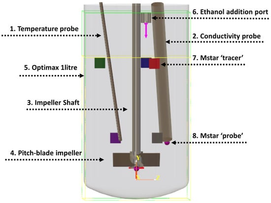
Figure 2.
Representation of the mixing vessel and probes used for M-star modelling. Probe and tracer injection locations correspond to those used experimentally. Dimensions correspond to those detailed in Table 1. The coloured squares represent tracer injection locations used in the simulations to investigate the effect of tracer addition location on mixing time. These are labelled as follows: 1. green, 2. blue, 3. red, 4. purple, and 5. grey. Note that tracer injection location 2 was used for all premixed simulations. Ethanol addition port refers to the addition of 200 mL of ethanol to the water in the solvent mixing simulations. Yellow line shows initial liquid height for a volume of 1 L, which was used for the premixed simulations. The light green box indicates the simulated geometry volume.
Five tracer injection locations (shown as coloured squares in Figure 2) were added to evaluate whether mixing time variance was more sensitive to spatial differences at the additional point or to temporal variations in the local velocity field at a fixed position. These locations were chosen to give a good sample, with three positions at the surface (green, blue, and red) and two near the impeller (purple and grey). The additional time-delayed injection at location 3 (red) allowed a assessment of how the temporally fluctuating flow patterns characteristic of transitional regimes affect mixing times at an identical spatial position.
To investigate the effect of tracer injection location, additional simulations were run which included five tracers being injected at various locations. These are shown as squares in Figure 2, with the colour relating to the location of the tracer. These locations were chosen to represent typical regions where liquid feeds may enter the vessels, with three positions at the surface and two near the impeller. The additional time-delayed injection at location 3 allowed a determination of how changing flow patterns over time affect mixing at the same position. For all other simulations, tracer location 2 (red) was used to match that used experimentally. In the solvent mixing experiments, ethanol was poured into the vessel. To approximate this in the CFD model, we took the diameter of the ethanol stream to be 1 cm at an addition time of 4 s. The volumetric flow rate of ethanol was therefore 50 mL/s.
2.2.2. CFD Simulations
CFD simulations were performed using the commercial software package M-star CFD (3.3.96) [24]. M-Star CFD uses a Lattice–Boltzmann approach to solve the time-dependent Naiver–Stokes equation [25,26]. Here, the Boltzmann transport equation is solved to model the time-dependent molecular probability density function () in phase space . This is expressed through Equation (2).
where are the molecular velocity vectors, K denotes any external forces acting on the particles, and is the collision operator. describes the rate of change over time in the molecular probability density function for species f with respect to collisions with species f. This becomes complicated for an n-body system; however, it can be argued that the result of multi-body collisions is for local distributions to tend to an equilibrium distribution (). Equation (2) is then expressed through
where represents the relaxation time, which describes how quickly the local distribution relaxes to its equilibrium state. Viscosity is therefore related to the relaxation time, with a larger relaxation time corresponding to a higher viscosity. Macroscopic properties such as density or momentum can be calculated from the moments of the distribution function. In M-star, the molecular velocities were discretised into the velocity vector set D3Q19 [24], as this gave the best balance between stability and speed of solver.
For all simulations, the free surface model was selected. In this model, a free-slip boundary condition is imposed at the fluid surface, whilst the vessel walls are assumed to have no-slip boundary conditions. Fluid–impeller interactions are modelled using the immersed boundary method, which enforces a no-slip velocity along the surface of the impeller. The turbulence model used was the large eddy simulation (LES) model with the default Smagorinsky coefficient of 0.1. To ensure lattice density fluctuations were kept within 1%, time steps were chosen to obtain a Courant number of 0.01. A lattice spacing of 0.65 mm was used.
Viscosity of the fluid mixture was calculated through a user-defined function. This was in the form of a polynomial which was fitted to the literature data [27]. M-star assumes volume averaged density, which for our system gives a reasonable approximation with a maximum error of around 5%. Figure 3 shows the properties of the fluid mixtures used here as a function of composition. Surface tension was taken from the literature for the solvent mixtures used [27].
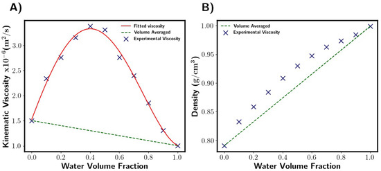
Figure 3.
Fluid properties as function of liquid composition [27]. (A) Viscosity. Fitted viscosity values are given by this polynomial: . M-star uses fitted viscosity function, whilst DynoChem uses volume-averaged (green dashed line). Note that Kinematic viscosity is shown. (B) Density. Both software packages assume density is volume-averaged. This gives a reasonable approximation with a maximum error of around 5% when compared to the experimental points (blue crosses).
2.3. Dynochem
We also used a mixing and heat transfer engineering toolbox from Dynochem, commonly used in industry, which is a spreadsheet-based software that employs empirical equations to estimate mixing times. The calculated mixing time is based on the time required to blend a tracer into the bulk such that it is 95% homogenised. The empirical correlations [28,29,30,31,32] used have been tested over a wide range of scales under different operating conditions with various impellers, and the typical error in the correlation under turbulent conditions is +/−14% [30]. For solvent mixtures, Dynochem assumes fluid properties, such as viscosity and density, are volume-averaged based on the solvent mixture composition used. In the transitional regime, this can lead to errors in systems such as water–ethanol mixtures, as viscosity is seen to significantly deviate from non-linear dependence on the solvent mixture fraction. See Appendix A for more details on Dynochem.
2.4. Mixing Time Characterisation
2.4.1. Experimental
Premixed solutions: We considered three mixing time estimation methods based on the conductivity profiles obtained from the probes, the 95% homogenisation method, and fitting exponential and first-order plus dead time models to the probe data. In all methods, conductivity profiles obtained from the tracer tests were used to characterise mixing times under varying conditions. Figure 6 demonstrates the mixing time definitions. In the 95% homogenisation method, the end of mixing was when the conductivity value was within +/−5% of the final steady state value. The final steady state value was taken as the plateau of the conductivity profile. The start of mixing was taken as the time in which the conductivity increase was first detected by the probe. To do this, a Savitzky–Golay filter was fitted to the conductivity data, and the first derivative with respect to time was calculated. This was then used to quantify the rate of change of conductivity within the system, allowing for the start of mixing to be estimated. The start of mixing was taken as when the derivative became greater than 0.1 , as this indicated a rapid increase in conductivity. For the other two methods of mixing time estimation, two equations were fitted to the conductivity profiles, the first of which was the exponential model:
where A is a fitted constant and represents the steady state conductivity value, and K is the time constant. A higher value of K corresponds to faster mixing time. The exponential function was fitted from the start of mixing. With the start of mixing being defined as described in the 95% homogenisation method.
The conductivity probes only detect the local conductivity at the probe location, resulting in a delay between the tracer being injected at the surface and an increase in conductivity being realised. In order to account for this and avoid estimating the start of mixing, a first-order plus dead time model (FOPDT) was fitted to the conductivity profiles.
In Equation (5), A is a fitted constant, again representing the steady state conductivity. is the delay time, whilst K is the time constant. From both of these equations, the time for 95% homogenisation was calculated, allowing for comparison with the 95% homogenisation method.
Mixing Solvents: We used the same approach as for premixed solvents with one additional consideration. When solvents are mixed together, heat is released due to enthalpy of mixing, which leads to a temperature increase of the solvent mixture. Although the vessel was temperature controlled, temperature measurements indicated an increase during mixing. Conductivity is a function of temperature, and thus, this was accounted for through a temperature calibration model. Details are shown in Appendix B.
2.4.2. Computational
Premixed solvents: Mixing times obtained by M-star were characterised using two different mixing indexes, with both being based on the tracer concentration. Firstly, the relative standard deviation (RSD) of the tracer concentration (mol/litre) was calculated to measure the overall degree of mixing within the vessel. In this work, we considered the system to be fully homogenised when the RSD value dropped below 5% [2,18]. Figure 4A shows RSD as a function of time, with the green dashed line highlighting when mixing was determined to be complete.
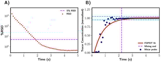
Figure 4.
Mixing time determination for premixed solvents using CFD. (A) Determination through relative standard deviation (RSD). Mixing was complete when the RSD of tracer concentration (% RSD) fell below 5%. This is indicated by magenta dashed line. (B) Determination via tracer concentration at probe location. Mixing time taken as the point in tracer concentration where values were within +/−5% of final steady state values. The +/−5% region is highlighted by blue dashed lines. The red line shows the FOPDT model fitted to the probe data. Magenta dashed line indicates the end point of mixing. Note that data were normalised with reference to the final tracer concentration after addition.
Although the RSD gives an good indication of the degree of mixing in a vessel, it does not offer a direct comparison to experimental results from this work. Experimentally, tracer concentration was measured using a conductivity probe, resulting in only localised conductivity profiles being readily available. In order to directly compare computational and experimental results, a probe was added to the CFD geometry in a position to match the experimental setup. This recorded the local tracer concentration every 0.1 s. The data were normalised with respect to the final fully mixed concentration of vessel. Mixing time was obtained when the variation in local concentration was within 5% of the final uniform concentration, i.e., 95% homogenisation. An exponential model (4) was fitted to the M-star probe data. Mixing time was then calculated for when this exponential fit would reach 0.95, i.e., 95% mixed.
To measure the variance of mixing times associated with each RPM and solvent mixture, four tracers were added during each simulation. The first of these was injected once the fluid flow in the vessel reached steady state. This time was based on preliminary simulation results. Subsequent tracers were then added at 3 s intervals. The injection location was kept constant for all tracers.
The effect of tracer addition location on mixing time was then investigated by adding five tracers to the vessel once steady state had been reached. This was location 3 at the fluid surface and location 2 close to the impeller. Tracer addition locations are shown in Figure 2.
Mixing of solvents: The same approach used as described above for premixed solvents. In place of tracer concentration, the volume fraction of ethanol was used to calculate RSD and the variation in the probe method. Addition of ethanol was assumed to take place over 4 s to match the experimental procedure.
3. Results and Discussion
3.1. Mixing Times in Water
3.1.1. Computational
In this section, we detail the mixing time characterisation techniques used in this work, which were applied to pure water systems. Firstly, we discuss the M-star CFD simulations, in which we considered two indicators of tracer homogeneity within the vessel: the relative standard deviation (RSD) of the tracer concentration and the local concentration values at the probe. In all analyses of the probe concentrations, we normalised the data with respect to the fully mixed tracer concentration. Figure 4 shows a representation of these mixing characterisation techniques applied to typical results obtained from M-star, %RSD, and M-star probe data. A first-order plus dead time model (Equation (5)) was fitted to the probe data, as shown by the red line in Figure 4B. The fitted FOPDT function was used to calculate the time required for mixing to be 95% complete. Mixing times were determined for all simulations using these three characterisation techniques, allowing for a comparison between the different methods.
A summary of the mixing times from M-star is shown in Figure 5. For these examples, we considered a pure water system. To investigate the variance in mixing times, tracer addition was repeated four times for each RPM simulated, with the injection location kept constant. The first tracer was added after a steady state had been reached, with subsequent additions taking place at 3 s intervals. To focus on variability between trials, only one method is shown in Figure 5A,B. Although we present this figure using % RSD, the same variability between trials was seen regardless of the estimation method used.
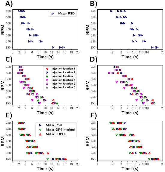
Figure 5.
Summary of mixing times calculated from M-star CFD for the pure water system. (A,B) Mixing times as characterised by the RSD method. Variance in mixing times highlighted by the spread of mixing times obtained at each RPM. (C,D) Effect of tracer injection location on determined mixing times. Location numbers are shown in the CFD geometry section. Injection location 3 refers to the same location as 2, but the injection of tracer was delayed by 3 s. Mixing times were determined using the RSD method. (E,F) Comparison of the three mixing time characterisation methods. The methods were used to determine mixing times for the same CFD simulations.
Inspecting the mixing times, the expected trend was observed, with an approximately inverse relationship between the mixing times and the impeller. Upon comparing the mixing times for individual trials, a variance between trials was revealed. From this, it becomes clear that the time required for homogenisation should not be considered as a single, deterministic time but rather as a range of values. This highlights the necessity in using multiple repeats of tracer addition to accurately capture the variability and spread of mixing times for the given process conditions.
The variance in mixing times can be explained by considering the local velocity profiles and flow pattern at the time and location of the tracer injection. In both the transitional and turbulent regime, the localised flow was significantly different at the same location in the vessel but a second apart. Thus, dispersion of the tracer within the fluid can be influenced by both the tracer location and time of addition. These effects were investigated by repeating the simulations performed previously, but with five different tracer addition locations used. A sixth tracer was added, at location 3, but with a two-second time delay. Tracer location 2 refers to the experimental location and that used for all other simulations. The exact locations for the tracer injections are shown in Figure 2. In the simulations, the tracer did not interact with the solvent mixture and followed the local fluid streamlines. Figure 5C,D summarises the results of this study.
The experiments revealed a similar variability in the mixing times across different tracer injection locations comparable to the variability observed in tracer repeat tests (see Figure 5A). This suggests that in the system studied, the injection location does not strongly affect the variance in mixing times. Notably, the mixing times for injections at the surface and close to the impeller were indistinguishable, although we note that only one trial was conducted for each location. This further demonstrates that the mixing time depends on the vessel fluid velocity field, which was inherently unstable under the transitional flow regime studied here. This instability explains the variability in the mixing behaviour across the vessel, regardless of the specific injection point.
Three methods were used to characterise mixing, which are compared in Figure 5E,F. Blue is the tracer RSD, green is the 95% homogenisation method, and red is the FOPDT model fitted to the M-star probe data. Using the % RSD provides an indication of the overall degree of tracer homogeneity within the vessel, whilst the probe only provides localised information. It can be argued that the % RSD gives a better representation of global mixing times, as probe measurements are influenced by position and as such do not take into account the homogeneity throughout the vessel. For example, regions in which mixing is poor within a vessel might suggest longer mixing times. It is not practical to measure the % RSD of the tracer experimentally, and so probes are regularly employed. From the simulations, we found that the average times calcuated by the % RSD method seem to be marginally longer than those determined from the M-star probe. This suggests that the probe may slightly underestimate the global mixing time, as reported in the work by Oblak [2] and discussed in Section 1. Although if we consider the distribution of mixing times, we see that both characterisation methods showed a similar variance in determined mixing times under the given conditions. This indicates that the distribution of calculated mixing times are consistent across the characterisation methods used. Assuming that a representative location is chosen for the probe, that despite only measuring localised variables, the probes are capable of capturing the global variability of the system to a reasonable extent.
3.1.2. Experimental
Similarly to the M-star CFD simulations, the three mixing time estimation methods were applied to the data obtained from the tracer experiments; see Figure 6. Figure 6A represents the typical conductivity profile of the tracer tests in premixed solvent mixtures. The green lines indicate when the probe detected the change in local conductivity. This was taken to be the start of mixing. One limitation of using probes is that the time between tracer addition and probe detection is not considered. The magenta lines indicate the end of the mixing using the 95% homogenisation method. The steady state conductivity value was taken as the plateau value of the conductivity. Although the majority of conductivity profiles behaved as shown in Figure 6A, there were a few where the conductivity did not settle to a uniform value. In these cases, the end of mixing was defined as when the oscillations were within 5% of the peak value of the increase in conductivity upon addition of the tracer.


Figure 6.
Experimental mixing time characterisation. (A) Typical conductivity profile obtained from the tracer experiments. (B) Example of conductivity profile which did not reach a steady state plateau. Green and magenta lines indicate the detection of tracer addition and the determined end of mixing. (C) Example of an exponential decay function being fitted to the experimental data. (D) Example of the first-order plus dead time model being fitted to experimental data. Both (C,D) were fitted to data at 450 RPM.
Figure 6C,D show that the exponential and first-order plus dead time (FOPDT) models fit to the experimental conductivity data. The exponential model was fitted to the increase in conductivity, with the start being defined as when the derivative of the conductivity with respect to time was greater than 0.1 . This corresponds to the steady state conductivity value and was taken as a fitted parameter alongside the time constant. As previously mentioned, the 95% homogenisation method did not account for the time delay between tracer injection and detection. To account for this, a FOPDT model was fitted to the data, with the time delay () used as a fitted parameter. As with the exponential model, the time constant and the steady state conductivity value were fitted parameters as well.
The experimental mixing times were characterised using the 95% homogenisation method using the conductivity profiles obtained from the probes. This is shown in Figure 7. As with the CFD simulations, variance was recorded across repetitions at all RPM values. The mixing times can be seen to clearly decrease as the RPM was raised from 150 to 350 RPM. Further increases in the RPM did not seem to significantly effect the mixing times, and a large variance was observed. A sodium chloride solution was used as the tracer, and the mixing times could potentially be limited by the break-up and dispersion of the tracer solution droplet in the vessel. A larger relative variance was observed at higher RPMs in comparison to lower RPMs. The calculated impeller Reynolds numbers indicated that for all RPMs used here, the vessels were in the transitional regime or the lower end of the turbulent regime, with Re numbers ranging from 5000 to 25,000. At these Reynolds numbers, the flow structures were highly unstable and small experimental perturbations, such as minor variations in the addition of the tracer, could have some impact on the mixing time measurement results. On the other hand, the computational investigation of the effect of the injection location reported in Figure 5C seems to indicate that the corresponding variability in the estimated mixing times is relatively small.
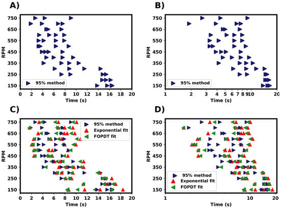
Figure 7.
Summary of mixing times determined from the experimental results for pure water. (A,B) Mixing times determined from the 95% homogenisation method. (C,D) Comparison of mixing time estimation methods from the same experimental results.
The fitted exponential and FOPDT models were compared to the 95% homogenisation method, as in Figure 7C,D. All three methods produced a similar spread of mixing times. For both fitted equations, the final steady state conductivity was taken as a fitted parameter. With the 95% based on this value, there would be differences in the end definition of mixing. In most cases, the difference between these were minimal. In the FOPDT model, the start of mixing was taken as a fitted parameter via the time delay constant (). This accounts for the delay in tracer addition and probe detection. These were found to be typically in the magnitude of 0.1–1 s. The inclusion of time delay can assist in relating the localised mixing time to the global mixing time of the vessel. The mixing times estimated by the FOPDT model seem to be marginally longer than those measured by the 95% homogenisation method. However, the overall distribution of mixing times was similar for all the three methods used and comparable to the results from the CFD simulations.
3.1.3. Comparison of Computational and Experimental Mixing Times
Figure 8 shows a comparison of the mixing times for the 1 L vessel as determined by the M-star CFD simulations, experimental tracer tests, and Dynochem calculations. Dynochem uses empirical equations based on the vessel geometry and fluid properties and, as a consequence, gives a single value for a given set of conditions and variability that therefore cannot be represented. Despite this, Dynochem gave a reasonable estimation of the mixing time in comparison with those determined experimentally and predicted by CFD simulations. Both the experimental and CFD results showed a significant variability in mixing times; however, two differences can be seen: larger variances and longer mixing times were seen in the experimental compared to the simulation results. A factor that may influence variability across experiments is the reproducibility of the tracer addition. In the CFD simulations, the tracer was added identically each time. One effect not captured by the CFD is the physical injection of the tracer, i.e., the tracer hitting the surface of the liquid, and the initial dispersion and breaking up of the tracer solution (sodium chloride in water). In the CFD simulation, the tracer was added just beneath the surface of the fluid, i.e., there were no surface tension effects. The tracer addition was perfectly reproduced across every simulated run, and consequently, there was no variability in the addition presented. In the simulations, the tracer used assumes no interaction between tracer and fluid, and its dispersion is only dependent on local fluid streamlines. We also note that values of tracer concentration measured by the simulated probe may not always accurately represent the experimental conductivity probe. For example, the interaction between sodium chloride and a physical probe is likely to differ from a simulated probe that measures the exact concentration at a point in the CFD system. These factors can result in the underestimation of the mixing times seen in our simulation results. Nonetheless, the simulated probe provides a reasonable approximation of the mixing times the under conditions investigated here.
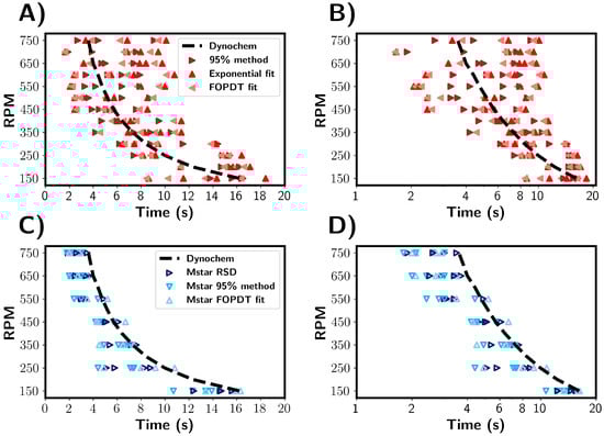
Figure 8.
Comparison of mixing times estimated from experimental and simulated data across a range of RPM values. (A,B) Mixing times estimated from experimental results. (C,D) Mixing times estimated from CFD simulations. The black dashed line depicts mixing times predicted by Dynochem.
To further investigate the tracer behaviour, we compared the local tracer concentration from the CFD simulations and the experimental conductivity as determined by their respective probes. We normalised these values to provide a better comparison between the two variables, and we define the time scales in terms of the number of impeller rotations. In Figure 9, the experimental and CFD data are depicted in red and blue shades respectively, with trial referring to the tracer addition repetition. The conductivity profiles from the experimental tracer tests were found to follow a distinct pattern. Initially, the conductivity gradually increased before a further sharper rise was observed. This was followed by one or more kinks in the conductivity profile until the final plateau was reached. This can be qualitatively related to the physical mixing process, as the tracer is injected at the liquid surface and starts to disperse into the vessel, corresponding to the initially slow increase in conductivity. The tracer was then drawn towards the impeller, the rate of dispersion increases, and a sharp rise in conductivity is seen. As the tracer moves to the liquid surface, dispersion rate reduces. Subsequently, the tracer will be drawn back into the impeller and the process continues until the homogenisation of tracer within the vessel is achieved. Some of the normalised concentration values exceeded unity, which is expected, since a small amount of highly concentrated tracer fluid is injected into the vessel, and regions of fluid with a higher tracer concentration may pass by the probe during the mixing process before homogenisation is completed.
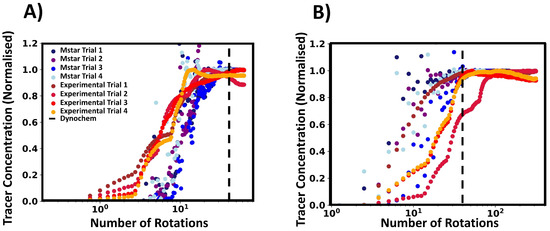
Figure 9.
Conductivity and tracer profiles (both normalised) plotted against number of impeller rotations. Red shades indicate experimental results, and blue shades show M-star probe data. (A) is for 150 RPM and (B) is for 750 RPM. The black dashed line indicates the number of rotations estimated by Dynochem. Note that Dynochem esimated an approximate constant number of rotations regardless of RPM.
The M-star probe shows that the tracer in the simulations behaves in a different manner than the tracer behaviour observed experimentally. Figure 9 gives a representative example of data at low RPMs (A) and high RPMs (B). At low RPMs, the tracer concentration increased in a exponential manner, with slight overshoots before reaching a steady state value. For higher RPMs, the data increased in an oscillatory way and then settled down to the steady state concentration. The contrast between the probe measurements and simulated tracer behaviour may offer a possible explanation for the differences in measured mixing times and the associated variances.
Following the comparison of the simulated and experimental probe tracer measurements, we present the estimated mixing times in terms of the number of impeller rotations in Figure 10. We can see that approximately the same number of impeller rotation was required for 95% homogenisation for each RPM. As expected from the mixing correlations from Dynochem, the mixing time was found to be inversely proportional to the rotational rate. For the CFD simulations (Figure 10C,D), we see a similar result, with the range of rotations being approximately 20–40 across all RPMs. This indicates that there is a small range of impeller rotations required to disperse the tracer throughout the vessel and achieve homogenisation of the tracer. Experimentally, the variance in impeller rotations was observed to widen with increasing RPM. Table 3 summarises the range of impeller rotations required to achieve reactor homogeneity within the vessel.
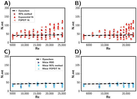
Figure 10.
Mixing times represented as the number of impeller rotations expressed as N.mt. Mixing times (mt) are shown as a function of impeller Reynolds number (A,B) Mixing times estimated from experimental results. (C,D) Mixing times estimated through CFD simulations. The black dashed lines depict mixing times predicted by Dynochem.
Table 3.
Mean mixing times expressed as number of impeller rotations for experimental and M-star CFD methods, along with Dynochem predictions. The brackets indicate the standard deviations for the corresponding number of rotations. Exp fit and FOPDT refer to exponential and first-order plus dead time model, respectively. Note that Dynochem gives single value for mixing time, and therefore, no standard deviation is given.
3.2. Premixed Water/Ethanol Solvent Mixtures
In the previous section, the mixing times for the pure water system were investigated in detail using a combined CFD and experimental approach. Multiple characterisation and estimation techniques were compared and discussed. Here, a comparison was made between premixed water/ethanol solvent mixtures of varying compositions. By premixed, we refer to the solutions being fully mixed prior to tracer addition. Regarding the characterisation method, the mixing times estimated from the experimental and CFD probe measurements were compared with those estimated from Dynochem in Figure 11. Firstly, the mixing times calculated by Dynochem (black dashed line) are shown in Figure 11. They reveal that a small increase in the mixing time occurred with increasing ethanol concentration at low RPMs due to increased solution viscosity. At higher RPMs, the Reynolds number became greater, and role of viscosity was diminished. Consequently, there was little effect on the calculated mixing times generated by Dynochem.
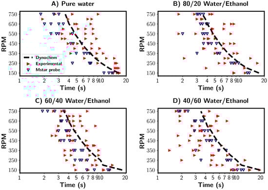
Figure 11.
Summary of mixing times for four different solvent compositions. (A) Pure water, (B) 80/20% v/v water/ethanol, (C) 60/40% v/v water/ethanol, (D) 40/60% v/v water/ethanol. Blue and red triangles depict mixing times from M-star probe and experimental probe, respectively. Both used the 95% homogenisation characterisation method. The black lines indicate mixing times calculated by Dynochem.
The experimental results are depicted by the red triangles in Figure 11. Across all solvent compositions, we see a relevantly large variance between the measured mixing times. The mixing times were longest for the pure water system, whilst they were shortest for the 40/60 water/ethanol % v/v mixtures. The calculated Reynolds numbers were found to be highest for pure water and lower for water/ethanol mixtures for the same RPM. This corresponds to increased viscosity in the water/ethanol mixtures. We thus see the unexpected trend of increased mixing times with higher Reynolds numbers. One possible explanation for this that the density of the solvent mixture decreased as ethanol volume fraction increased. With the tracer composition being constant, the density difference between the tracer and solvent increases with increasing ethanol content. A higher difference may lead to the tracer being pulled towards the impeller and broken up quicker, reducing the mixing time. Tracer/solvent interactions could also play a role in the mixing times.
The CFD simulations (blue triangles) showed no clear trends between the mixing time and solvent composition. Variations in the mixing times were seen for all solvent compositions, and a similar trend to those discussed in the previous sections was found. In comparison to the experimental results, where tracer/solvent density differences were the suggested possible explanation, this would not be taken into account in the simulations in which the tracer is a passive participant in the mixing process.
3.3. Solvent Mixing
To investigate the injection of the antisolvent into a solution as occurs in antisolvent crystallisation processes, the mixing times were estimated for the addition of ethanol to water. The results are summarised in Figure 12. Firstly, the mixing times are discussed in units of seconds, as shown in Figure 12A,B. Experimentally, the ethanol was added rapidly through a vessel inlet port, and it was estimated that this process took about 4 s. In the times predicted by the CFD simulations, a plateau was reached at around 4 s, suggesting that the ethanol addition was the rate-limiting step. Experimentally, mixing times shorter than 4 s were observed, indicating that the assumed time for ethanol may have been shorter than 4 s. This makes the comparison between the computational and experimental results more qualitative than quantitative. As with premixed solutions, the simulated probe tended to underestimate the global mixing, as described by the RSD. Note that instead of the tracer concentration, the ethanol volume fraction was used to estimate the mixing time for the CFD simulations.
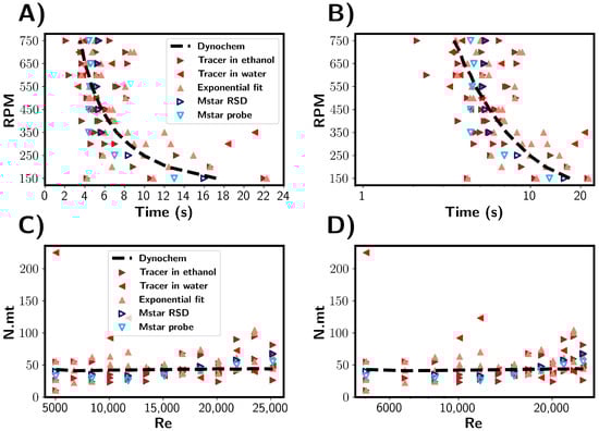
Figure 12.
(A,B) Comparison of experimental and CFD estimated mixing times for the addition of ethanol/tracer mixtures to water. Blue and red symbols depict experimental and simulated results, respectively. (C,D) Mixing times corresponding to (A,B) shown in number of rotations, expressed as N.mt. Mixing times are shown as a function of impeller Reynolds number.
During the experimental tracer tests, the salt tracer location was varied. Three repeats per RPM were performed in which the tracer was initially located in ethanol, and one experiment per RPM was performed in which the salt tracer was located in water prior to ethanol addition. At RPMs above 350 RPM, we found the mixing times to fall approximately within the 2–10 s band, with the variance similar across the RPMs. With 200 mL of ethanol being added as opposed to 10 mL of tracer, there is a greater potential for variability in the tracer injection process, e.g., injection time, location, and ethanol stream diameter. The minimum mixing time would be limited by the time taken for ethanol to be added, so it can be expected that above a certain RPM there would be no further decrease in the mixing time, as can be seen in Figure 10. However, the mixing times were found not to be dependent on the initial tracer location.
Figure 12C,D show mixing times in reference to the number of rotations. Experimentally, the rotations needed was in the range 25–60, which is comparable to the premixed solvent systems discussed above. In the CFD simulations where the mixing time was limited by the ethanol addition, it is seen that 0 rotations were required for mixing to achieved. This increased because the minimum time was limited by the ethanol addition rate; thus, more rotations occur at higher RPMs.
The conductivity profiles recorded by the conductivity probe are shown in Figure 13. The data shown are representative of typical data acquired for (A) high RPMs and (B) low RPMs. For high RPMs, the conductivity profile followed a similar pattern to the premixed systems, with kinks observed in the profile. Again, this can be attributed to the ethanol/tracer mixture initially dispersing at the fluid surface. As it is drawn towards the impeller, it is dispersed into the water rapidly, and a sharp conductivity increase is observed. At low RPMs, the initial conductivity profiles look similar to those at higher values. However, a plateau was not reached, and it was not possible to accurately determine the end of mixing due to conductivity oscillations. At very long time scales, the observed oscillations reduced; however, a steady state value was not achieved within the recorded time frame. From the mixing times characterised in the premixed systems, we can infer that the approximate times for lower RPMs would be lower than 30 s, and one would not expect the long mixing times indicated by the probe data.
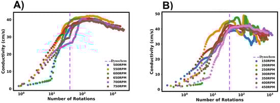
Figure 13.
Conductivity vs. number of impeller rotations for the addition of ethanol to water. (A) shows high RPMs, whilst (B) shows low RPMs.
This study highlights the fundamental variability of flow fields in the transitional regime, demonstrating that variations in mixing times are inherently part of the mixing process rather than being just due to methodological limitations. The significant run-to-run variability observed across both the experimental and simulation approaches reflects the stochastic nature of transitional flow, where fluid structures fluctuate unpredictably between more laminar-like and turbulent-like states.
3.4. Limitations and Future Works
Some limitations should be taken into account when considering the results of this study. On the computational side, tracers for water and premixed water–ethanol solutions were modelled as ideal volumes being dispersed by following local fluid streamlines, while the addition of ethanol to water was modelled as a dispersion of ethanol in water, where the salt tracer was assumed to disperse alongside the ethanol. The modelled tracers for water and premixed water–ethanol solutions were added just beneath the fluid surface, eliminating possible droplet breakage and surface tension effects present in experiments, where the tracer solution was injected from above at the solution surface. Furthermore, probe implementation in CFD simulations may not fully represent the responses of the conductivity probe to the local salt tracer concentration. These simplifications may have contributed to underestimation of the mixing times and their variability compared to experimental measurements.
On the experimental side, the reliance on a single conductivity probe in the experimental setup provided only local concentration measurements that may not fully represent the global mixing state within the vessel. While single-probe-based methods are commonly used for practical reasons, they inherently sacrifice spatial resolution and can underestimate the actual mixing times if placed in regions that mix more rapidly than others. Interestingly, the CFD simulations showed that the RSD-based mixing times (representing global mixing) were slightly longer than the probe-based measurements, though the uncertainty ranges overlapped substantially, suggesting that suitably positioned single-point measurements can provide reasonable approximations of global mixing times.
While some degree of variability in mixing time is inherent due to the stochastic nature of flow fields in the transitional regime, future work could focus on reducing potential methodological uncertainties. The tracer addition process could be automated to ensure consistent delivery in terms of injection location, volume, speed. and direction. Multiple conductivity probe positions throughout the vessel could be explored to provide a more representative picture of global mixing patterns compared to the single-point measurements employed in this study. CFD model refinements could include incorporating more realistic tracer–fluid interactions and surface tension effects to better represent experimental conditions.
From a scale-up perspective, the approach presented here shows good potential for scale up using established chemical engineering principles. For example, expressing mixing times in terms of impeller rotations and Reynolds numbers provides a basis for scaling equations that could be applied across different vessel sizes. The combined experimental and CFD approach demonstrates that while reasonable predictions of mean mixing times can be made by various methods, the inherent variability in mixing times can be expected to persist at larger scales and should be accounted for in process design. Future work should include validation at different scales to confirm the applicability of these findings in other systems.
4. Conclusions
The mixing times were estimated for a miscible liquid systems in a one-litre agitated vessel utilising a combined experimental and CFD approach. Experimentally, tracer tests were performed using sodium chloride tracer and measuring conductivity profiles using a conductivity probe. Three characterisation methods were applied to the measured conductivity profiles, namely, the 95% homogenisation method, fitting exponential, and first-order plus dead time models. This was then simulated using CFD, with the mixing times also estimated using the % relative standard deviation of the tracer within the vessel. An M-star probe was simulated to represent the physical measurement, with the 95% homogenisation method being applied to the tracer concentration profiles obtained. Lastly, Dynochem was used to estimate the mixing times using empirical correlations. Across all mixing characterisation methods, the estimated times were found to be within 1–20 s, with higher impeller RPMs corresponding to shorter mixing times. The mixing time were found to be approximately inversely proportional to the impeller RPM, as expected from empirical correlations.
Multiple tracer additions allowed for the variability in the mixing times to be quantified. Both the experimental and CFD methods showed a wide variance in mixing times. A larger variance in the mixing times was observed experimentally in comparison to those predicted by CFD. This could be due to more variance being involved in the physical addition of the experimental tracer or the CFD not fully capturing other physical effects. Nevertheless, all characterisation methods point to variability being inherent to mixing processes. One implication of this is that although empirical correlations such as those used in the Dynochem empirical correlations can give a reasonable estimation of the mixing times, they do not capture their inherent variability.
By noting that mixing times are inversely proportional to impeller speed, we can express the mixing time in terms of the number of impeller rotations required for solution homogenisation. For M-star CFD, it was found that a narrow range of impeller rotations (5–40) was required for blending, with this being independent of the RPM. Experimentally, a larger range of impeller rotation was needed (25–100). In comparison, Dynochem predicted 0 impeller rotations for homogenisation, independent of the RPM.
The effect of solvent composition on the mixing time was investigated by repeating simulated and experimental tracer tests for various water/ethanol mixtures. The simulated mixing times did not show a significant difference between solvent compositions, whilst experimentally, the mixing times were found to decrease with increased ethanol content in the solvent mixture. Lastly, the mixing times for antisolvent addition were estimated by injecting 200 mL of ethanol into 800 mL of water. Experimentally, the mixing time was determined to plateau at RPMs above 350 RPM, with the measured variance being consistent. The mixing times appeared to be limited by the ethanol addition rate; thus, further increasing the RPM would have little effect on the resulting mixing times.
This study demonstrated and quantified the inherent variability of mixing times in the transitional flow regime in a mixed solvent system relevant for antisolvent crystallisation. Despite some limitations in both the experimental and computational approaches, including simplified tracer behaviour in the CFD simulations and localised probe measurements, the findings provide valuable insight into water–ethanol mixing within the transitional flow regime at the one-litre scale. Future research could focus on the validation of these findings at other scales and enhancement of CFD model fidelity through incorporation of realistic tracer–fluid interactions and surface tension effects to better represent experimental conditions.
Author Contributions
Conceptualisation, J.S., N.N. and L.L.; methodology, J.S., N.N., R.M. and L.L.; software, R.M.; validation, J.S., N.N. and L.L.; formal analysis, R.M. and I.C.B.; investigation, R.M. amd I.C.B.; resources, J.S. and N.N.; data curation, R.M. and I.C.B.; writing—original draft preparation, R.M. and I.C.B.; writing—review and editing, J.S. and R.M.; visualisation, R.M. and J.S.; supervision, J.S., N.N. and L.L.; project administration, J.S. and N.N.; funding acquisition, J.S. and N.N. All authors have read and agreed to the published version of the manuscript.
Funding
This research was funded by the EPSRC and the Future Manufacturing Research Hub in Continuous Manufacturing and Advanced Crystallisation (Grant ref: EP/P006965/1).
Data Availability Statement
The data are confidential.
Acknowledgments
The authors would like to thank Chris Mitchel for his contribution in providing assistance with the experimental work.
Conflicts of Interest
The authors declare no conflicts of interest.
Appendix A. Dynochem
A mixing and heat transfer toolbox and a spreadsheet-based software from Dynochem were used to estimate the mixing time. The calculated mixing time is based on the time required to blend a tracer into the bulk such that the additive is 95% homogenised. The mixing time correlations for the turbulent (Equation (A1)) and transitional (Equation (A2)) regime are given as such [28,29,30,31,32]:
where is the mixing time (s), is the power per unit volume (kW/m3), T is the tank diameter (m), D is the impeller diameter (m), is the liquid viscosity (Pa s), H is the liquid height (m), V is the liquid volume (m3), and is the liquid density (kg/m3). N represents the impeller rotational speed (1/s). The power input P (W) is calculated using Equation (A3), with a power number () dependent on the impeller choice. From this, the power per unit volume () is calculated, i.e., . In the turbulent regime, it is seen that the mixing time () is inversely proportional to N, the impeller speed. In the transitional regime, () is inversely proportional N2.
DynoChem assumes that the tracer has similar physical properties (i.e., density and viscosity) to the bulk. The correlations are valid for both turbulent and transitional phases, but not for the laminar phase. Note that Re is the impeller Reynolds number given by Equation (A4), where is the density (kg/m3), N is the impeller rotation speed (s−1), D is the impeller diameter (m), and is the dynamic viscosity of the liquid phase.
The correlations used have been tested over a wide range of scales at different operating conditions with different impellers, and the typical error in the turbulent correlation is +/−14% [30]. For solvent mixtures, Dynochem assumes fluid properties are a volume average of the solvents used—in this case, water and ethanol. Figure 3 (main article) shows the viscosity and density used. Table A1 shows the parameters used within the Dynochem toolbox.
Table A1.
Table of parameters used in Dynochem calculations. The range corresponds to the various water/ethanol compositions.
Table A1.
Table of parameters used in Dynochem calculations. The range corresponds to the various water/ethanol compositions.
| Parameter | Nomenclature | Value |
|---|---|---|
| Tank diameter | T | 101 mm |
| Impeller diameter | D | 45 mm |
| Dynamic Viscosity | 1.14–1 mPas | |
| Impeller speed | N | 150–750 RPM |
| Liquid density | 914–1000 kg/m3 | |
| Liquid height | H | 0.135 m |
| Liquid Volume | V | 1 L |
| Power number | Po | 1 |
Appendix B. Temperature Calibration for Conductivity Probe
During the mixing of 200 mL of ethanol with water, enthalpy due to mixing is released, resulting in a temperature increase of the system. Although the reactor had temperature control, a temperature increase was noticed. Conductivity is a function of temperature, and it is therefore dependent on the temperature of the vessel. To account for this, a calibration model was fitted. Conductivity was measured at five temperatures; 15, 20, 25, 30, and 35 °C. Figure A1 shows the obtained conductivity profile.

Figure A1.
Conductivity profile obtained during temperature calibration of the conductivity probe. Left and right y axes show temperature and conductivity, respectively.
Figure A1.
Conductivity profile obtained during temperature calibration of the conductivity probe. Left and right y axes show temperature and conductivity, respectively.

After each temperature increase, a conductivity increase followed before it reached the new equilibrium value. Oscillation were found to occur, which increased with the temperature of the water. An average value was taken as an estimation of the conductivity. A straight line function was found to describe the system well and was selected for the calibration model. The conductivity was then corrected before the mixing times were calculated.
Appendix C. Mixing Time Characterisation—Typical Data
The mixing times were calculated using the definition given in the Methods section. Figure A2 shows typical data acquired. (A) depicts the conductivity profile. The green dashed line indicates the start of mixing, which is defined as when the derivative of conductivity increases above 0.1. The corresponding derivatives are shown below in (B). The end of mixing is is when the conductivity value is within 5% of the final steady state value. This is depicted by the purple dashed line. Temperature correction was done using the temperature calibration model developed in the previous section.

Figure A2.
Mixing determination for experimental data. (A) The criteria for ‘fully’ mixed is the same as for premixed solvents, i.e., when the step increase is within +/−5% of the final value (conductivity). The green and magenta line indicate the start and end of mixing, respectively. (B) Mixing profile plotted on conductivity vs number of impeller rotations. (C) First derivative of conductivity profile with respect to time. This was calculated from Savitzky–Golay filter fitted to data from (A). (D) Temperature calibration curve was calculated using experimental data. This accounts for temperature differences during mixing.

Appendix D. Premixed Solvent Comparison—Averaged Mixing Times
The average mixing times are shown for different water/ethanol mixtures. We see that the experiential mixing time decreased with increasing ethanol fraction, whilst the simulated results were found to be largely independent of the solvent composition.

Figure A3.
Average mixing time values compared for different solvent compositions. Ratios in legend are given on a percent volume basis. (A) Experimental results. (B) M-star CFD. In both, magenta line represents Dynochem calculations calculated for pure water.
Figure A3.
Average mixing time values compared for different solvent compositions. Ratios in legend are given on a percent volume basis. (A) Experimental results. (B) M-star CFD. In both, magenta line represents Dynochem calculations calculated for pure water.

References
- Harnby, N.; Edwards, M.; Nienow, A. Mixing in the Process Industries; Butterworth Heinemann: Oxford, UK, 1985. [Google Scholar]
- Oblak, B.; Babnik, S.; Erklavec-Zajec, V.; Likozar, B.; Pohar, A. Processes Digital Twinning Process for Stirred Tank Reactors/Separation Unit Operations through Tandem Experimental/Computational Fluid Dynamics (CFD) Simulations. Processes 2020, 8, 1511. [Google Scholar] [CrossRef]
- Al-Qaessi, F.; Abu-Farah, L. Prediction of Mixing Time for Miscible Liquids by CFD Simulation in Semi-Batch and Batch Reactors. Eng. Appl. Comput. Fluid Mech. 2009, 3, 135–146. [Google Scholar] [CrossRef][Green Version]
- Martinetz, M.C.; Kaiser, F.; Kellner, M.; Schlosser, D.; Lange, A.; Brueckner-Pichler, M.; Brocard, C.; Šoóš, M. Hybrid Approach for Mixing Time Characterization and Scale-Up in Geometrical Nonsimilar Stirred Vessels Equipped with Eccentric Multi-Impeller Systems-An Industrial Perspective. Processes 2021, 9, 880. [Google Scholar] [CrossRef]
- Cabaret, F.; Bonnot, S.; Fradette, L.; Tanguy, P.A. Mixing Time Analysis Using Colorimetric Methods and Image Processing. Ind. Eng. Chem. Res. 2007, 46, 5032–5042. [Google Scholar] [CrossRef]
- Ascanio, G. Mixing Time in Stirred Vessels: A Review of Experimental Techniques. Chem. Eng. Res. Des. 2015, 23, 1065–1076. [Google Scholar] [CrossRef]
- Holmes, D.B.; Voncken, R.M.; Dekker, J.A. Fluid Flow in Turbine-Stirred, Baffled Tanks-I. Circulation Time. Chem. Eng. Sci. 1964, 19, 201–208. [Google Scholar] [CrossRef]
- Arratia, P.E.; Muzzio, F.J. Planar Laser-Induced Fluorescence Method for Analysis of Mixing in Laminar Flows. Ind. Eng. Chem. Res. 2004, 43, 6557–6568. [Google Scholar] [CrossRef]
- Kling, K.; Mewes, D. Two-Colour Laser Induced Fluorescence for the Quantification of Micro- and Macromixing in Stirred Vessels. Chem. Eng. Sci. 2004, 59, 1523–1528. [Google Scholar] [CrossRef]
- Delaplace, G.; Bouvier, L.; Moreau, A.; Guérin, R.; Leuliet, J.C. Determination of Mixing Time by Colourimetric Diagnosis—Application to a New Mixing System. Exp. Fluids 2004, 36, 437–443. [Google Scholar] [CrossRef]
- Kraume, M.; Zehner, P. Experience with Experimental Standards for Measurements of Various Parameters in Stirred Tanks: A Comparative Test. Chem. Eng. Res. Des. 2001, 79, 811–818. [Google Scholar] [CrossRef]
- Lee, K.C.; Yianneskis, M. A Liquid Crystal Thermographic Technique for the Measurement of Mixing Characteristics in Stirred Vessels. Chem. Eng. Res. Des. 1997, 75, 746–754. [Google Scholar] [CrossRef]
- Nere, N.K.; Patwardhan, A.W.; Joshi, J.B. Liquid-Phase Mixing in Stirred Vessels: Turbulent Flow Regime. Ind. Eng. Chem. Res. 2003, 42, 2661–2698. [Google Scholar] [CrossRef]
- Sardeshpande, M.V.; Kumar, G.; Aditya, T.; Ranade, V.V. Mixing Studies in Unbaffled Stirred Tank Reactor Using Electrical Resistance Tomography. Flow Meas. Instrum. 2016, 47, 110–121. [Google Scholar] [CrossRef]
- Harrison, S.T.; Stevenson, R.; Cilliers, J.J. Assessing Solids Concentration Homogeneity in Rushton-Agitated Slurry Reactors Using Electrical Resistance Tomography. Chem. Eng. Sci. 2012, 71, 392–399. [Google Scholar] [CrossRef]
- Tan, C.; Dong, F.; Hua, S. Gas-Liquid Two-Phase Flow Measurement with Dual-Plane ERT System in Vertical Pipes. AIP Conf. Proc. 2007, 914, 3. [Google Scholar] [CrossRef]
- Bach, C.; Yang, J.; Larsson, H.; Stocks, S.M.; Gernaey, K.V.; Albaek, M.O.; Krühne, U. Evaluation of Mixing and Mass Transfer in a Stirred Pilot Scale Bioreactor Utilizing CFD. Chem. Eng. Sci. 2017, 171, 19–26. [Google Scholar] [CrossRef]
- Nguyen, D.; Rasmuson, A.; Björn, I.N.; Thalberg, K. CFD Simulation of Transient Particle Mixing in a High Shear Mixer. Powder Technol. 2014, 258, 324–330. [Google Scholar] [CrossRef]
- Bouwmans, I.; Van den Akker, H. The Influence of Viscosity and Density Differences on Mixing Times in Stirred Vessels. IChemE Symp. Ser. 1990, 121, 1–12. [Google Scholar]
- Mirfasihi, S.; Basu, W.; Martin, P.; Kowalski, A.; Fonte, C.P.; Keshmiri, A. Investigation of mixing miscible liquids with high viscosity contrasts in turbulently stirred vessels using electrical resistance tomography. Chem. Eng. J. 2024, 486, 149712. [Google Scholar] [CrossRef]
- Mirfasihi, S.; Basu, W.; Martin, P.; Kowalski, A.; Fonte, C.P.; Keshmiri, A. A numerical study on the mixing time prediction of miscible liquids with high viscosity ratios in turbulently stirred vessels. Chem. Eng. Sci. 2025, 304, 120944. [Google Scholar] [CrossRef]
- Derksen, J. Blending of miscible liquids with different densities starting from a stratified state. Comput. Fluids 2011, 50, 35–45. [Google Scholar] [CrossRef]
- Madhania, S.; Cahyani, A.B.; Nurtono, T.; Muharam, Y.; Winardi, S.; Purwanto, W.W. CFD study of mixing miscible liquid with high viscosity difference in a stirred tank. IOP Conf. Ser. Mater. Sci. Eng. 2018, 316, 012014. [Google Scholar] [CrossRef]
- M-Star. M-Star CFD (Version 3.3.96). 2025. Available online: https://www.mstarcfd.com/. (accessed on 1 April 2025).
- Succi, S. The Lattice Boltzmann Equation for Fluid Dynamics and Beyond; Clarendon Press: Oxford, UK, 2001; p. 288. [Google Scholar]
- Guo, Z.; Shu, C. Lattice Boltzmann Method and Its Applications in Engineering; World Scientific: Singapore, 2013. [Google Scholar]
- Khattab, I.S.; Bandarkar, F.; Fakhree, M.A.A.; Jouyban, A. Density, viscosity, and surface tension of water+ethanol mixtures from 293 to 323 K. Korean J. Chem. Eng. 2012, 29, 812–817. [Google Scholar] [CrossRef]
- Li, J. Effect of Impeller Type and Number and Liquid Level on Turbulent Blend Time. Ph.D. Thesis, University of Dayton, Dayton, OH, USA, 2017. [Google Scholar]
- Hicks, R.; Morton, J.; Fenic, J.G. How to Design Agitators for Desired Process Response. Chem. Eng. J. 1976, 83, 102–110. [Google Scholar]
- Greenville, R.; Ruszkowski, S.; Garred, E. Blending of Miscible Liquids in the Turbulent and Transitional Regimes. In Proceedings of the Mixing XV: 15th Biennial North American Mixing Conference, Banff, AB, Canada, 18–23 June 1995. [Google Scholar]
- Zhao, D. Liquid Macro- and Micro-Mixing in Sparged and Boiling Stirred Tank Reactors. Ph.D. Thesis, University of Surrey, Guildford, UK, 2002. [Google Scholar]
- Hardy, N.; Augier, F.; Nienow, A.W.; Béal, C.; Chaabane, F.B. Scale-Up Agitation Criteria for Trichoderma Reesei Fermentation. Chem. Eng. Sci. 2017, 172, 158–168. [Google Scholar] [CrossRef]


Disclaimer/Publisher’s Note: The statements, opinions and data contained in all publications are solely those of the individual author(s) and contributor(s) and not of MDPI and/or the editor(s). MDPI and/or the editor(s) disclaim responsibility for any injury to people or property resulting from any ideas, methods, instructions or products referred to in the content. |
© 2025 by the authors. Licensee MDPI, Basel, Switzerland. This article is an open access article distributed under the terms and conditions of the Creative Commons Attribution (CC BY) license (https://creativecommons.org/licenses/by/4.0/).