1. Introduction
Computational fluid dynamics (CFD) is the solution of partial differential equations of fluid mechanics obtained by approximating them through linear algebraic equations using finite difference or finite volume methods and solving the resulting system by numerical schemes and with the aid of a computer [
1]. The methodologies employed to attain this solution are categorized into three principal groups: finite difference methods, finite volume methods, and finite element methods. Finite difference methods are employed in conjunction with structured meshes, whereas finite volume methods are utilized for unstructured meshes [
1,
2].
One field in which the application of CFD has proven particularly fruitful is the petroleum industry. The processing of crude oil necessitates the involvement of numerous processes, wherein the transfer of mass and energy and the conversion of chemical species are of utmost importance. The flow of fluids is a fundamental operation in this industry as the transformation of mass requires the flow of raw materials. These materials may be transported through a pipeline or processed into equipment that exchanges energy or transforms them into products of higher value. This transformation may occur through a change in chemical composition or the elimination of compounds for environmental reasons [
3].
The final category encompasses the catalytic hydrotreating (HDT) of petroleum distillates, which serves the purpose of eliminating sulfur, nitrogen, and oxygen compounds. Such compounds would otherwise be transformed into environmental pollutants when the fuel is burned. To enhance the efficacy of the HDT process, it is imperative to determine the flow profiles of the gas–liquid (hydrogen–hydrocarbon) mixture at the inlet disperser section above the upper distributor plate and throughout the catalytic bed.
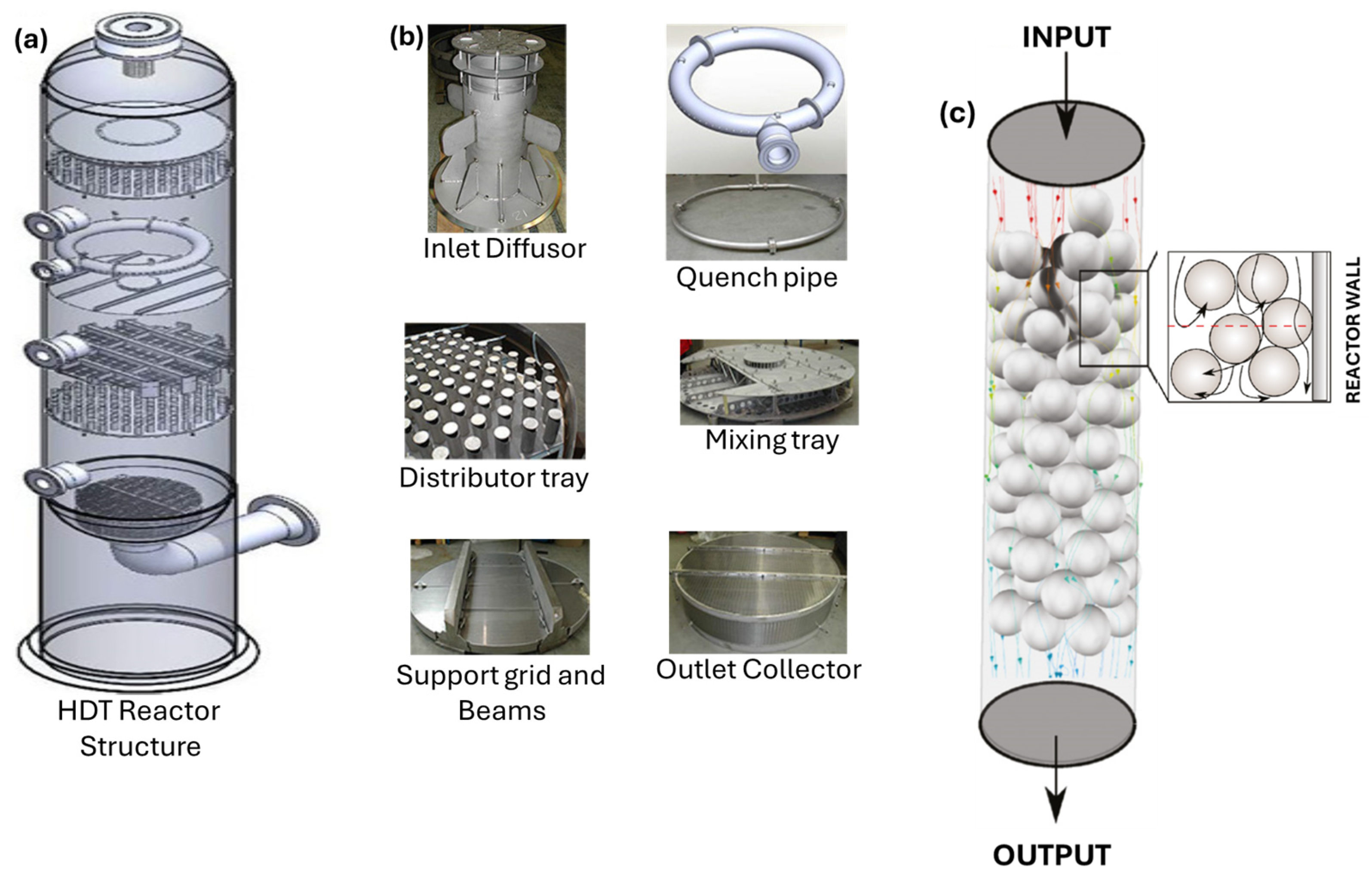
The complexity of the geometry of each component through which the gas–liquid mixture flows is a challenge to simulate using CFD, as can be seen in
Figure 1a, where the general layout of a HDT reactor is shown.
Figure 1b shows the reactor internals through which the reacting two-phase mixture flows.
Figure 1c illustrates a schematic representation of the packed bed, which shows that it is formed by a large amount of catalyst particles with an average size of 1.6 mm in diameter, placed randomly.
The inlet disperser and the upper distributor plate are more straightforward to simulate than the packed bed as their geometries feature well-defined margins that can be adequately represented in the drawings. In contrast, the catalytic bed, comprising a bed of catalyst in granular form randomly loaded into the reactor, presents a more challenging geometry for CFD simulation. However, approximations have been made using porous media or by simulating the flow through a limited group of catalyst particles [
4].
The methodologies employed in CFD simulations of HDT reactor sections vary significantly, largely due to the inherent geometric complexities of each section. Simulations of sections where the flow is through a pipe, such as the loading section, are relatively simple. This is because the flow is a two-phase gas–liquid flow through a pipe, which can be simulated without significant difficulty. The flow through the diffuser to the discharge of the load feed pipe presents a greater challenge as it is a two-phase gas–liquid flow that must traverse a series of bulkheads, which attenuate turbulence to enable the flow to reach the subsequent stage: the distributor plate. However, the staggered placement of the bulkheads represents a greater complexity of the geometry, as well as a change in the flow pattern, which transitions from a fully turbulent flow to an almost laminar flow. The subsequent structure of interest within the hydrotreating reactor is the distributor plate. This device is responsible for distributing the gas–liquid mixture in a way that ensures the downstream flow is as homogeneous as possible, which in turn improves the distribution of the mixture through the catalytic bed. As indicated by its name, the distributor plate is tasked with the distribution of the fluids. The CFD simulation of the distributor plate represents the most complex aspect of reactor structure given the considerable range of sizes involved. The discrepancy in scale between the various geometries introduces a significant challenge to the CFD simulation procedure.
In most cases where the distributor plate has been simulated, simplifications have been made to reduce the complexity of the calculations. Such techniques facilitate the design, mesh creation, and convergence of the simulation, although they may result in a certain degree of loss of rigor. Nevertheless, these approaches yield valuable insights for the analysis, design, and optimization of distributor plates.
As the packed catalytic bed represents the most crucial component of the HDT reactor, it is also the area that has been most extensively examined using CFD simulations. Nevertheless, due to its multi-scale nature, it is not feasible to conduct a comprehensive simulation of the entire geometry, at least with the techniques and computational resources currently accessible at the academic level. Accordingly, this section of the reactor has been approached by simplifying the geometry of both the bed length and the size and number of catalytic particles involved, which represents the most rigorous form of approximation. Nevertheless, the prevalent methodology for simulating a packed bed is to conceptualize it as a porous medium. A CFD simulation should be carried out with the utmost rigor, with the geometry considered at a 1:1 scale. However, the number of meshes required to define the computational domain grows exponentially, making it unfeasible to define the mesh from the outset. Furthermore, the convergence stage is characterized by an immense computational capacity due to the number of nodes to be simulated. This often results in either an unachievable convergence or an unfeasible computation time. It remains appropriate to perform representative simplifications of each of the elements of the hydrotreating reactor; however, it is essential to define the simplified geometry to ensure that the results are suitable for analysis, design, or optimization tools.
Considering the role that the HDT process plays in oil refineries, particularly in the production of ultra-low-sulfur diesel, this paper presents a comprehensive review of the latest research where CFD simulation has been employed to examine the various sections of a trickle-flow reactor. This paper describes the models applied in the CFD simulation and discusses the results obtained with respect to the available experimental data.
Although CFD has already been used for several years and has been applied to a large number of situations, both in general and in several scenarios of Science and Engineering, specifically in Process Engineering, this has not been the case for the HDT process for the production of ultra-low-sulfur diesel (ULSD), which is why an analysis and discussion of this state-of-the-art process, as reported in the literature, is necessary. From this, the procedures that were followed to implement such simulations are highlighted.
First, the main structures inside a HDT reactor are established: inlet pipe, diffusor, main distributor tray, secondary distributor tray, packed bed(s), redistributor tray, and outlet collector. Likewise, it is established that the sections that influence the development of the HDT reactions are the former five structures mentioned above; so, the present study focuses exclusively on the CFD simulation work for these sections. Different drag models are also included, as well as turbulence models applicable in general and in particular to the CFD simulation of the HDT reactor.
A background on CFD simulations applied to the ULS Diesel HDT process is provided, as well as the history of the development and theoretical foundations since the year 2000. For CFD simulation works for the HDT process, the period of the published literature is from 2015 to date. A detailed description and an analysis of the results obtained are discussed, where the benefits and limitations of the CFD simulations are established.
To date, CFD simulations of HDT reactor sections for ultra-low-sulfur diesel production have been performed through simplifications in both the size and complexity of the systems. For purely mechanical sections that do not involve considerable differences in dimensions, it is feasible to implement the simulation directly, whereas for those with large differences, special considerations must be made to allow for a transition of the discretization, which in turn permits the calculation procedure to be stable. For sections that include granular material, such as the packed catalytic bed, to date, it is necessary to simulate them as a porous medium or by only simulating a few granular particles inside a small cylinder. Fortunately, there are now models and calculation procedures that make it possible to adequately handle situations where dimensions with considerably different sizes are present, although they can also be treated by considering symmetrical systems, which simplifies the calculations.
Regarding packed beds, more research is needed to develop procedures and models that allow treatment as a formal packed bed, although due to the notable difference between the dimensions of the container and the dimensions of the catalyst particles, it is practically impossible to simulate a full-scale system, even if it were possible to count on enormous computational resources that are highly expensive and which are only normally found in large research institutes or in large companies that produce machinery and equipment for the oil industry.
CFD simulation has been used for the analysis, design, and optimization of several general and specialized situations but not for all operations, processes, and equipment of the oil industry or as a regular tool for the HDT process of oil fractions, which is why it is relevant to establish its importance to improve all aspects of this process.
Although it is true that artificial intelligence (AI) is currently emerging as an integration option for CFD simulation, it is only being used for very simple systems and situations; so, there are no CFD simulation investigations with integrated AI for the simulation of the HDT process and are thus not included in this work.
The HDT process is of great importance within the oil refining industry, and the main equipment of this process is the reactor that comprises the aforementioned sections, which are feasible to be optimized with two main objectives: to meet the specification of the impurity content of the product and to improve the utilization of the catalyst.
The optimization of these sections by carrying out experiments is impractical and costly since it is necessary to develop a prototype for each of the cases to be evaluated. This is why the use of computational tools, such as CFD, has emerged as a way of performing such optimizations since different computational prototypes can be developed in a faster and less expensive way.
This motivates the current review of the literature carried out for the analysis, design, and optimization of the different sections of the HDT reactors. Therefore, the objectives of this work are to describe the systems, models, and procedures used for such purposes and to analyze the reported results, establishing how much they reproduce the experimental results with which such studies are validated.
3. Description and Analysis of Selected Works on CFD Simulation of HDT Reactors
The HDT reactions carried out in the TBR are influenced by the operating conditions: pressure, temperature, H2/HC ratio, and space velocity. However, one of the most important physical aspects that influence both the performance of the HDT reactions and the lifetime of the catalyst is the hydrodynamic behavior of the gas–liquid flow through the main distributor plate, as well as the flow of the fluids across the catalytic bed. Nevertheless, to date, there has been a lack of research conducted on the effect of gas–liquid flow hydrodynamics on the behavior of HDT reactions. The following section presents a description of the most recent work in this field.
A Eulerian–Eulerian approximation was used in almost all the analyzed papers. Those that applied the Eulerian-Lagrangian approximation have been described in the research of Courtais et al. [
40]; the CFD-DEM approximation is mainly used to simulate a fluid–particle system, mainly those that handle a fluid–particle flow; so, it is not widely used for the simulation of gas–liquid flow in HDT reactors.
On the other hand, computational fluid dynamics (CFD) volume of fluid (VOF) theory is used to model multi-phase flows with distinct boundaries between phases. It is used in a variety of applications, including simulating the motion of bubbles, jet breakup, and liquid–gas interfaces. VOF theory is extensively employed to model multi-phase flows with distinct boundaries between phases, the motion of bubbles or large bubbles in a liquid, the motion of liquid after a dam break, the steady or transient tracking of any liquid–gas interface, free-surface laminar flows, jet disintegration phenomena, pool boiling, fluid fall (like a waterfall), and spillways.
The VOF method introduces an extra transport equation for each simulation with two fluids. This equation requires new boundary conditions and additional mesh refinements. The VOF method represents which fluid or fraction of both fluids occupies each cell in the mesh. Other applications include the modeling of bubble rising and coalescence in low holdup particle–liquid suspension systems. As can be seen, these systems do not correspond to the CFD simulation of the HDT reactors; so, this VOF theory is not applicable.
Neto et al. [
41] stated that it is necessary to know the detailed behavior of the HDT reactor to optimize its operation despite the scarcity of reports on these reactors. The research considered the mass transfer of gas–liquid and liquid–solid phases and the deactivation and quenching of the catalyst, which occur in conjunction with the plug flow observed in a diesel hydrotreater. A pseudo-component kinetic model was successfully used, and the average molar mass of each pseudo-component was obtained from the average molar mass of the feedstock.
Table 2 shows the stoichiometric coefficients of the reactions, while
Table 3 details the kinetic models and their parameters.
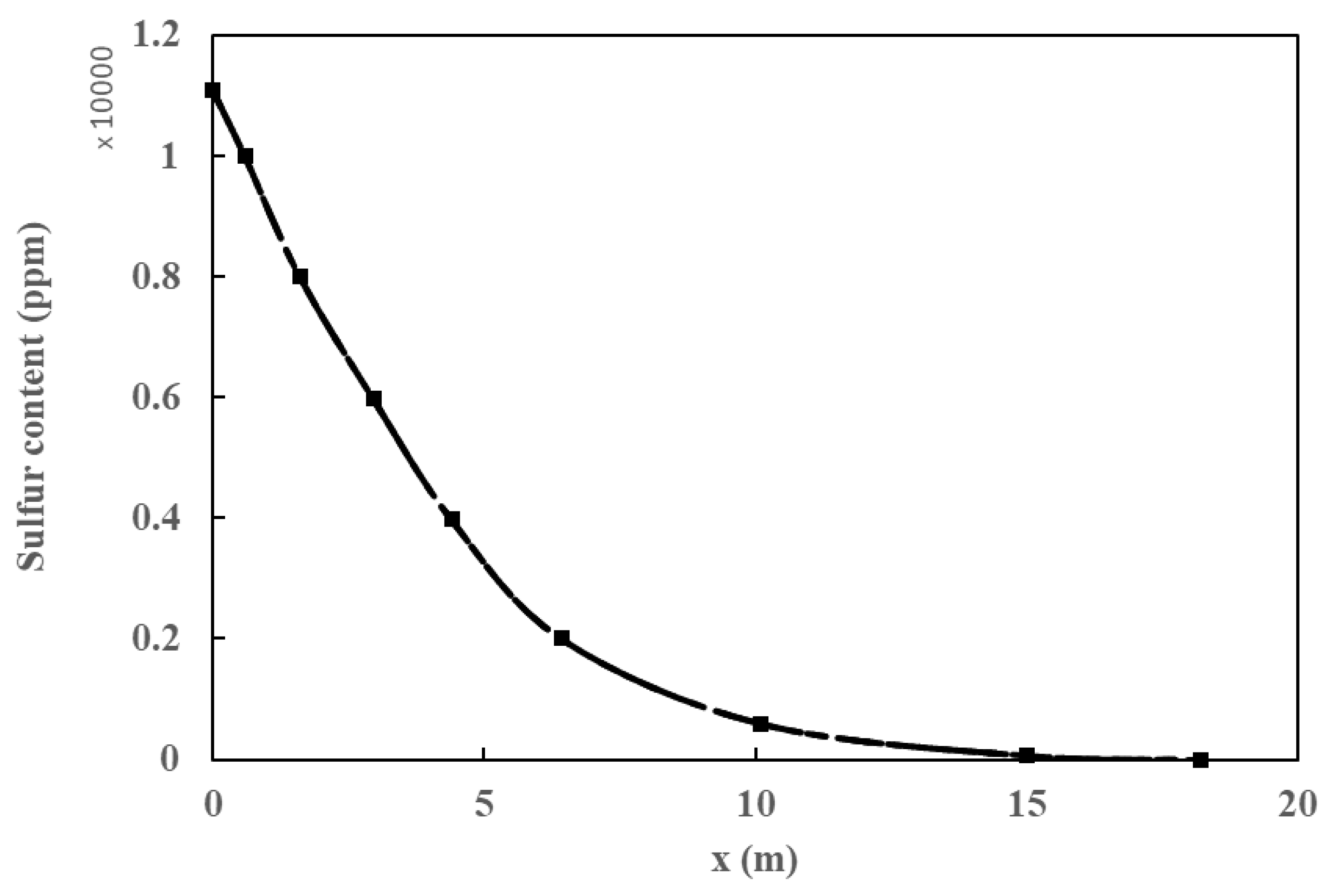
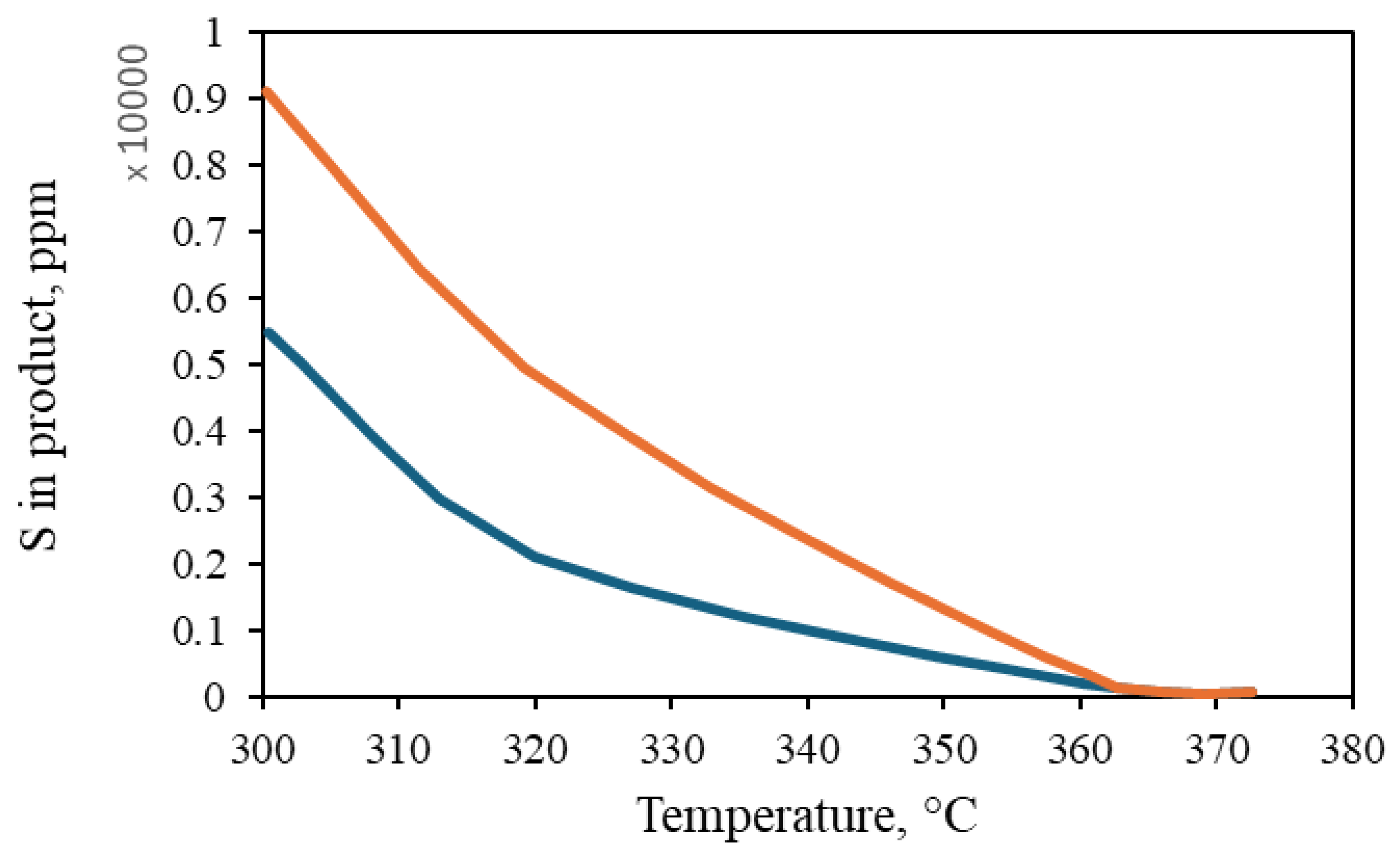
Both the plug flow model and the CFD simulation were validated with data obtained from industrial plants by analyzing the sulfur content and temperature profiles. There was a 14% deviation among simulations and experimental values (
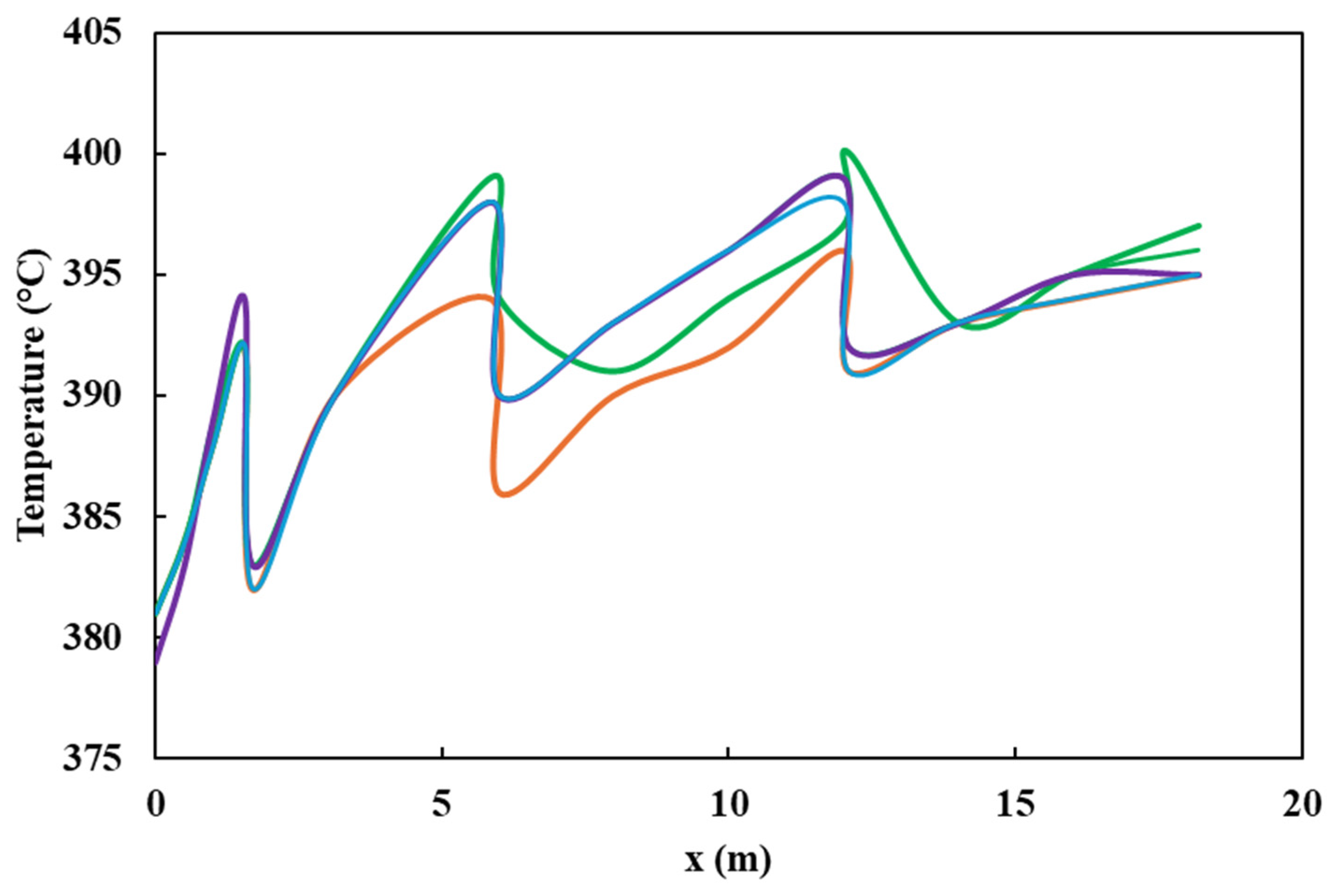
Figure 4). It is observed that both values overlap and follow the same trend. Furthermore, the impact of pressure and species distribution, in addition to the influence of inlet pressure and temperature on the ultimate sulfur content of the product, is discussed. In addition, the radial temperature profile obtained from the simulation at different heights of the HDT reactor is compared, as shown in
Figure 5, with a deviation of 1.1%. The small differences between the calculated and real data confirm that the various reactions taking place, such as hydrodesulfurization (HDS), hydrodenitrogenation of olefins (HOF), hydrodearomatization (HAD), and hydrocracking (HCC), were correctly modeled by the Langmuir–Hinshelwood kinetics model applied to an industrial reactor. The simulations were quite accurate due to the inclusion of catalyst deactivation in the prediction of the sulfur content of the products.
The main cause of catalyst deactivation is the deposition of coke, whose precursors are aromatics and olefins. In the catalyst deactivation model, each molecule of precursor consumed in the coking reaction is considered to produce one molecule of coke. Coke formation over time on the catalyst surface is given by:
where
is the molar concentration of coke on the catalyst surface and
corresponds to the molar concentration of coke precursor. This term is calculated as follows:
is the olefin concentration,
is the concentration of mono-aromatics,
is the concentration of diaromatics, and
is the concentration of poly-aromatics. A power-law model for coke formation can be established as follows:
where
is the rate constant for coke formation. In addition, the catalyst activity can be described by the following equation:
where
is the catalyst activity,
m and
n are parameters acquired from experimental data, and
is the coke amount calculated by:
represents the carbon-to-hydrogen ratio of hydrocarbon.
The injection of quench makes the temperature at the reactor outlet insensitive to catalyst activity. However, temperature does affect catalyst activity and conversion. The hydrotreating reactions are exothermic because the HDA reaction is one of the sources of heat that is used in the remaining reactions. Therefore, a complete set of reactions, including all HDT reactions, is mandatory to properly simulate the process.
Improvements in the reaction behavior are obtained when the bed is well packed with the catalyst. In their research, Courtais et al. [
40] employed geometry optimization to ascertain the optimal configuration of the packed bed in the reactor. The procedure was conducted by solving a multi-objective optimization problem, with consideration given to the concentration of products at the reactor outlet and the heat dissipation in the fluids. The equations of continuity, convection–diffusion, and Navier–Stokes were applied over an isovolumetric space and the reactor thicknesses, which were considered the constraints of the problem. The optimal reactor shape has been demonstrated to significantly enhance conversion by 12.6% in comparison to the initial geometry. Furthermore, it has been shown to facilitate a 3.5-fold increase in heat dissipation, thereby enabling more precise temperature control within the reactor. One of the most significant contributions of Courtais et al. [
40] is the clear demonstration of the necessity for a multi-objective optimization approach to the analysis of a catalytic reactor. Their findings indicated that when a single-objective methodology is employed, the optimal reactor design remains elusive. It must be acknowledged that even the multi-objective methodology has limitations that require further development, such as the thickness constraint resulting from post-processing the mesh displacement, which lacks rigor due to the Lagrangian approximation. It would be of significant interest to reformulate the constraints by penalizing the barrier functions in a manner that enables more optimal functionality, specifically through differentiability with respect to the domain. The second limitation pertains to the optimization approach of the form utilized, which precludes the formation or transformation of species within the reactor.
Another area in which computational fluid dynamics (CFD) can be employed is in the scale-up of reactors. Typically, all HDT process studies start in micro-reactors and subsequently progress to bench reactors, where the catalyst performance and operating conditions can be validated with a heightened level of confidence. Subsequently, the objective is to scale up to an industrial scale. The development of topological optimization techniques makes it possible to improve the geometry of the fixed-bed reactors.
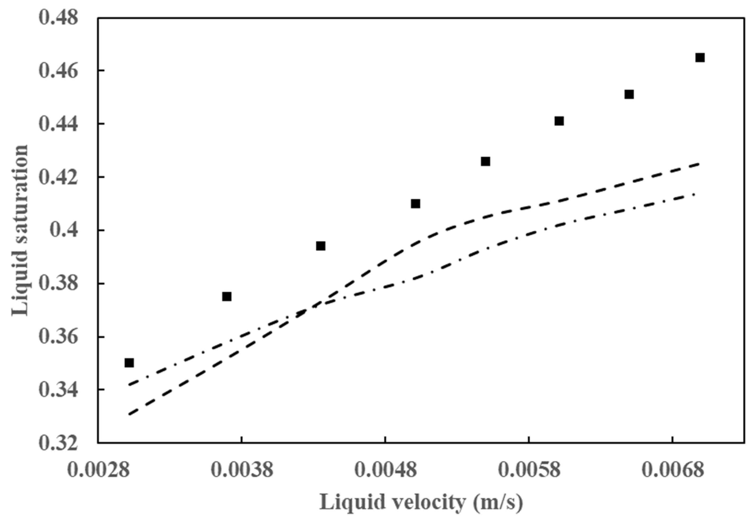
To gain insight into the behavior of a bench-scale HDT reactor, Abdolkarimi [
42] conducted a computational fluid dynamics simulation. As a primary assertion, the author posits that the scaling methodology performed via straightforward protocols frequently culminates in suboptimal reactor designs. Additionally, the fluid dynamics of trickle-flow hydrotreating reactors is intricate and highly susceptible to reactor scaling. The author employed a 2D CFD simulation based on a two-phase Eulerian model to investigate the performance of a bench HDT reactor. The packed bed was modeled using the porous media concept, and the resulting data were validated using reported data.
As has been demonstrated in numerous prior studies, a few factors, including poor flow distribution, channeling, catalyst wetting, and local temperature variation, exert control over the behavior of HDT reactors. In the analysis and design of HDT reactors, the two most crucial hydrodynamic parameters are pressure drop and liquid holdup. A comparison of the simulation results for these two parameters with experimental data is provided in
Figure 6 and
Figure 7.
Figure 6 illustrates the outcomes of the pressure drop analysis, whereas
Figure 7 depicts the mean liquid saturation values.
The application of computational fluid dynamics enables a comprehensive understanding of the fluid dynamics and its interaction with the kinetics of the process, facilitating a more rigorous analysis of the operating conditions. This, in turn, allows for the scaling up of the process with a higher degree of confidence. The pressure drop and liquid holdup for a bench reactor are predicted, and it is concluded that these results are in close agreement with the experimental data, as can be seen in
Figure 6 and
Figure 7.
In a previous study, Heidari and Hashemabadi [
44] proposed a Eulerian–Eulerian approximation to simulate the hydrotreating process (HDS and HDA) in a TBR using CFD. A tubular reactor with a length of 500 mm and a diameter of 19 mm was simulated. It consisted of a packed bed comprising three sections. Two particle sections, each with a diameter of 0.2 mm, were located at the end. The top section was 150 mm long, while the bottom section was 100 mm long. The reaction section, situated among them, had a length of 250 mm and employed trilobular catalyst particles with an average length of 3.5 mm and an average diameter of 1.6 mm. The kinetics of the HDS and HDA reactions were modified to include the influence of the porosity distribution, the non-isothermal conditions in the catalytic bed, and the effect of partial wettability on the kinetic constants of the reactions, as demonstrated in
Table 4. In addition, a gas–liquid interfacial heat transfer coefficient was employed to assess reactor behavior under isothermal conditions [
44]. The impact of the inlet temperature of the feed, gas and liquid velocities, operating pressure, and sulfur concentration in the gas phase were examined to ascertain the conversion of the reaction and the temperature distribution within the catalytic bed. The validation of the CFD model was conducted using the data reported by Chowdhury et al. [
45] at varying levels of porosity, assuming uniformity across the packed bed, fully wetted catalyst particles, and operation under isothermal conditions. These assumptions are detailed in
Table 5. The optimal values of the reaction constants for the HDS and HDA reactions, as determined through the bisection method, are presented in
Table 6. The CFD simulation results showed a discrepancy of 5.5% regarding the data published by Chowdhury et al. [
45].
The results demonstrate that the SDS prediction under adiabatic conditions is 9% higher than that predicted under isothermal conditions. Furthermore, it was observed that the prediction error of the CFD model for an SDS conversion increased by 5% with respect to the experimental data when the interfacial heat transfer coefficient was ignored. Additionally, the prediction of the flow patterns in the packed bed was also affected.
Gunjal and Ranade [
46] argued that the scaling of TBR reactors used in industry is a challenging process and that the application of simple scaling rules often results in unsuitable designs for the intended purpose; therefore, the authors used CFD to perform such scaling. Furthermore, it was demonstrated that the primary parameters governing the overall behavior of the HDT reactor were flow maldistribution, channeling, catalyst wetting, and packed bed temperature distribution. The fluid dynamics within HDT reactors is a highly complex phenomenon, exhibiting a high degree of sensitivity to the scaling procedure. Consequently, conventional modeling techniques are unable to adequately consider the key design parameters that have been previously identified. The advancement of CFD in recent years has already been recognized as a valuable technique for elucidating fluid dynamics and their impact on the chemical reactions involved in the HDT process.
In the study conducted by Gunjal and Ranade [
46], a CFD model was developed for a HDT reactor, both at the laboratory and commercial scales, in order to simulate the reactor flow field and HDT reactions. Once validated, the model was employed to elucidate the impact of catalyst bed porosity distribution, catalyst particle characteristics, and reactor scaling on the overall reactor performance. The validated model was employed to predict the behavior of the reactor at the commercial scale. The authors made a significant contribution to the knowledge of the complex interactions between hydrodynamics and chemical reactions in HDT, particularly in relation to the influence of reactor scale-ups on the behavior of the TBR reactor.
The CFD model for the TBR employed in the research conducted by Gunjal et al. [
43] comprised two distinct components: the porosity distribution within the catalytic bed, which is a function of both bed and particle characteristics, and flow model equations, which are based on the Eulerian–Eulerian multi-fluid model. The model provided information on fluid retention, pressure drop, and local fluid velocities, which is useful in reactor design and avoids uncertainties related to empirical correlations. Only the HDS and HDA reactions were considered, and the reactor conditions were previously reported by Chowdhury et al. [
45], while the kinetic equations and parameters were taken from Gunjal et al. [
43].
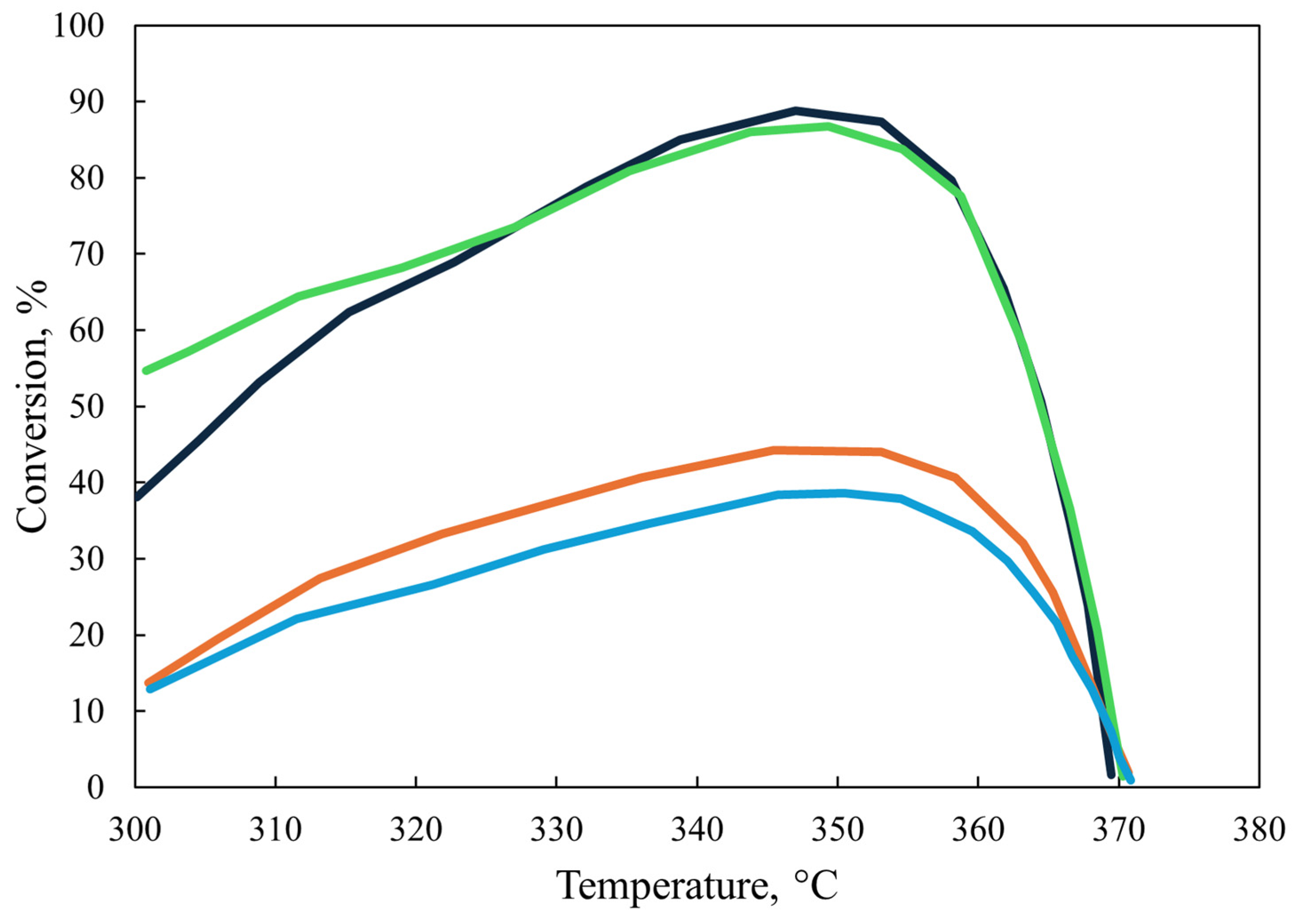
The configuration of the reactor components, including the distributor plate, reactor arrangement, bed packing method, local/total porosity distribution, catalyst particle size and shape, and plate configuration, affects the flow within the reactor. The inlet flow is uniformly distributed, while the flow of the gas–liquid mixture is primarily influenced by the shape and diameter of the catalyst particles, as well as their porosity and the diameter of the packed bed. The model is utilized to simulate the behavior of laboratory and industrial-scale reactors, with the objective of studying the influence of reactor size on reactor behavior. A comparison of the sulfur content among the laboratory and industrial reactors revealed that the concentration was lower in the laboratory-scale reactor, as illustrated in
Figure 8, whereas at higher temperatures, the behavior of the two reactors exhibited a high degree of similarity. As illustrated in
Figure 9, the conversion of poly- and mono-aromatic compounds for both reactors is nearly identical.
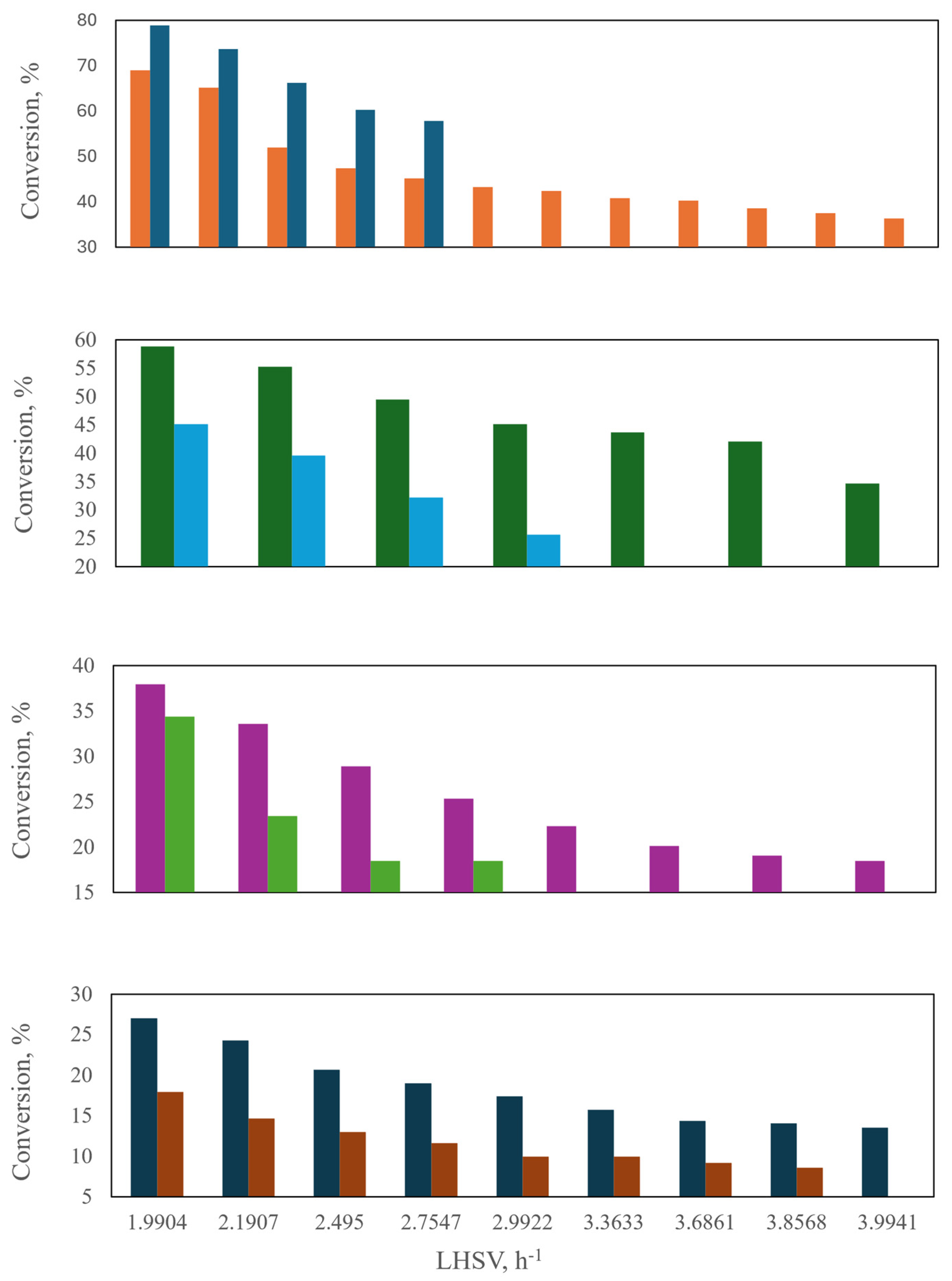
However, at 320 °C, the conversion of aromatic sulfur compounds in the two reactors exhibits a notable divergence with respect to the LHSV, as illustrated in
Figure 10. The conversion of these compounds declines in a gradual and uninterrupted manner at the laboratory scale. In contrast, the industrial reactor demonstrates a relatively constant conversion rate following an initial increase in the liquid flow rate (LHSV = 3 h
−1). This phenomenon may be attributed to the inhibition of flow caused by the elevated concentration of hydrogen sulfide in the industrial reactor, which allows for higher conversions to be attained.
Table 4.
Variation of operating parameters with respect to temperature [
4].
Table 4.
Variation of operating parameters with respect to temperature [
4].
| Cases | Tent (°C) | P(MPa) | LHSV | | |
|---|
| Sim T1 | 300 | 4 | 2 | 200 | 0.014 |
| Sim T2 | 320 | 4 | 2 | 200 | 0.014 |
| Sim T3 | 340 | 4 | 2 | 200 | 0.014 |
| Sim T4 | 380 | 4 | 2 | 200 | 0.014 |
| Sim P1 | 320 | 2 | 2 | 200 | 0.014 |
| Sim P2 | 320 | 4 | 2 | 200 | 0.014 |
| Sim P3 | 320 | 8 | 2 | 200 | 0.014 |
| Sim L1 | 320 | 4 | 1 | 200 | 0.014 |
| Sim L2 | 320 | 4 | 2 | 200 | 0.014 |
| Sim L3 | 320 | 4 | 4 | 200 | 0.014 |
| Sim Q1 | 320 | 4 | 2 | 100 | 0.014 |
| Sim Q2 | 320 | 4 | 2 | 200 | 0.014 |
| Sim Q3 | 320 | 4 | 2 | 300 | 0.014 |
| Sim Q4 | 320 | 4 | 2 | 500 | 0.014 |
| Sim H S12 | | 4 | 2 | 200 | 0 |
| Sim H2 S2 | | 4 | 2 | 200 | 0.014 |
| Sim H2 S3 | | 4 | 2 | 200 | 0.030 |
| Sim H2 S4 | | 4 | 2 | 200 | 0.080 |
Table 5.
Optimum values of reaction constants for HDS and HDA [
4].
Table 5.
Optimum values of reaction constants for HDS and HDA [
4].
| Reactions | Isothermal and Fully Wet Catalyst | Adiabatic and Partially Wet Catalyst |
|---|
| 2.5 × 10¹² | 7.166 × 10¹² |
| ) | 2.66 × 10⁵ | 4.23 × 10⁵ |
| ) | 8.5 × 10² | 1.33 × 10³ |
| ) | 6.04 × 10² | 9.62 × 10² |
Table 6.
Parameters of the case studies of Subramanian et al. [
47].
Table 6.
Parameters of the case studies of Subramanian et al. [
47].
| Case No. | Foam | Liquid Surface Velocity (ms)−1 | Surface Gas Velocity (ms)−1 |
|---|
| 1 | 20 ppi | 0.02 | 0.2 |
| 2 | 20 ppi | 0.03 | 0.2 |
| 3 | 20 ppi | 0.02 | 0.4 |
| 4 | 30 ppi | 0.02 | 0.2 |
| 5 | 30 ppi | 0.03 | 0.2 |
| 6 | 30 ppi | 0.02 | 0.4 |
At low liquid flow, the performance of both reactors for the hydrogenation of aromatic compounds is observed to be highly similar, as depicted in
Figure 11. The same trend is observed at high pressure, indicating that the effect of the gas concentration on the conversion of aromatic compounds is negligible. Nevertheless, at elevated liquid flow rates, reactor size has a significant influence, with the industrial reactor demonstrating superior performance compared to the laboratory-scale reactor, as observed in
Figure 12. The data presented in
Figure 8,
Figure 9,
Figure 10,
Figure 11 and
Figure 12 indicate that the performance of the industrial reactor is superior to that of the laboratory reactor. This phenomenon is particularly evident in the conversion of aromatic sulfur compounds, as observed in the study conducted by Rodriguez and Ancheyta [
48].
The direct interpretation of the results obtained presents a significant challenge. However, the use of CFD simulation offers a more direct and effective approach to analyzing and interpreting these results. It is therefore evident that CFD simulation is useful in visualizing the behavior of the reactors, thus enabling a deeper analysis of the data to perform the optimal configuration of the HDT reactor.
Uribe et al. [
49] conducted an analysis and optimization of the HDT process using a multi-physics and multi-scale approach. According to their criteria, this approach should be applied in many engineering cases and processes, representing a significant challenge in analysis and optimization tasks. Computational fluid dynamics offers a multi-scale approach that enables the precise establishment, understanding, and quantification of local and micro-scale phenomena, which significantly influence the overall behavior of the HDT reactor. The authors studied three cases: (i) a heterogeneous micropore model (HMM), (ii) a pseudo-homogeneous catalyst particle model (PCM), and (iii) a reactor scale model (RSM).
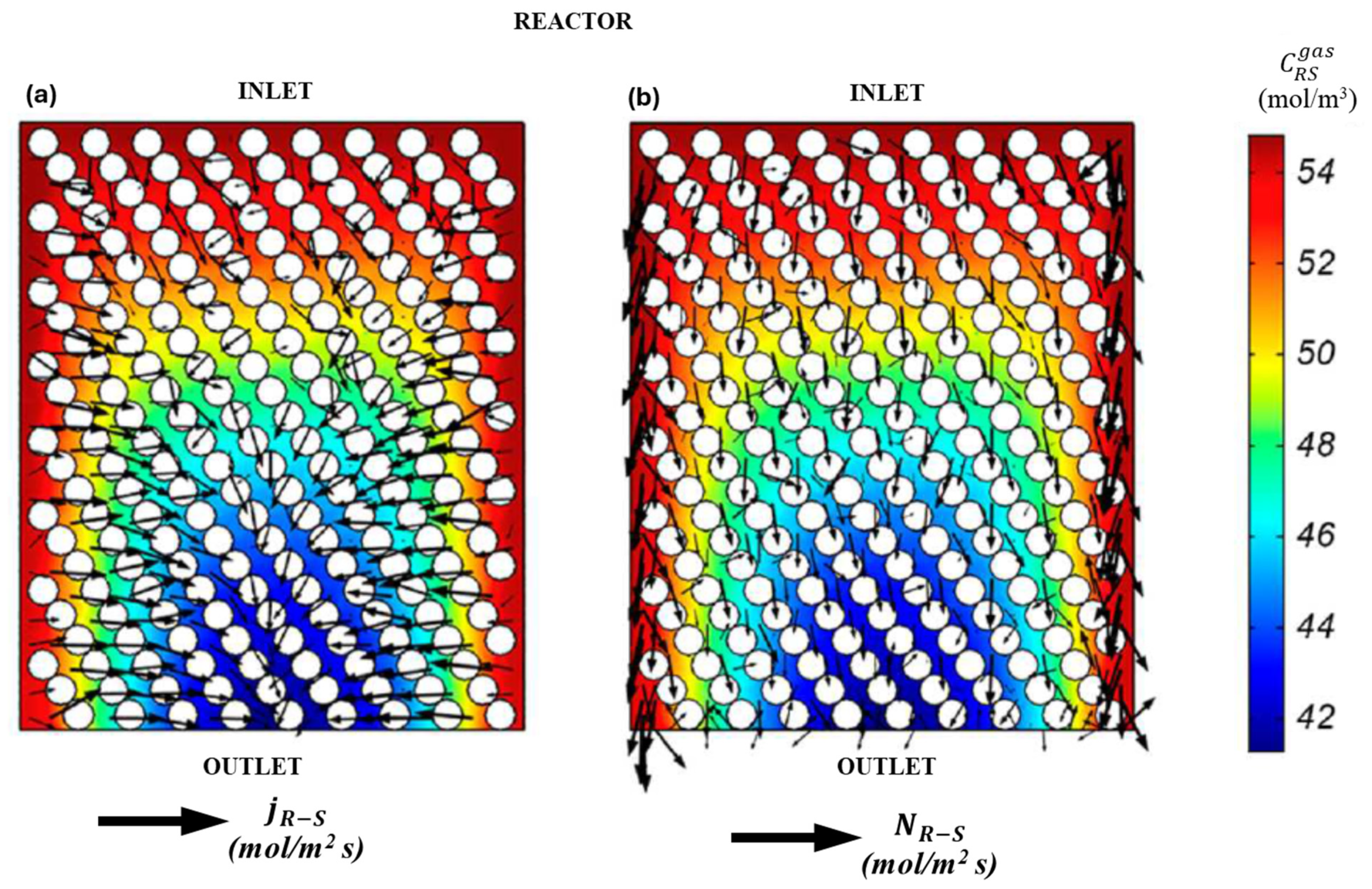
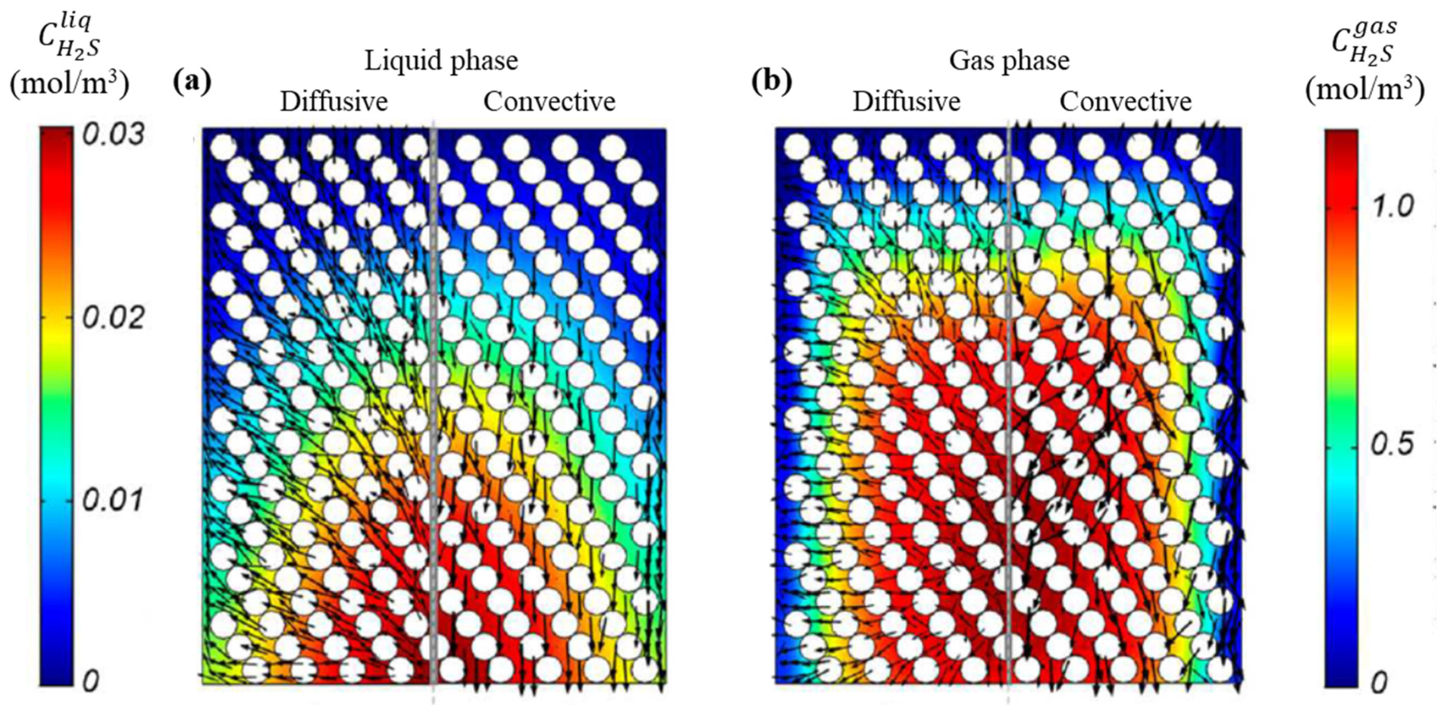
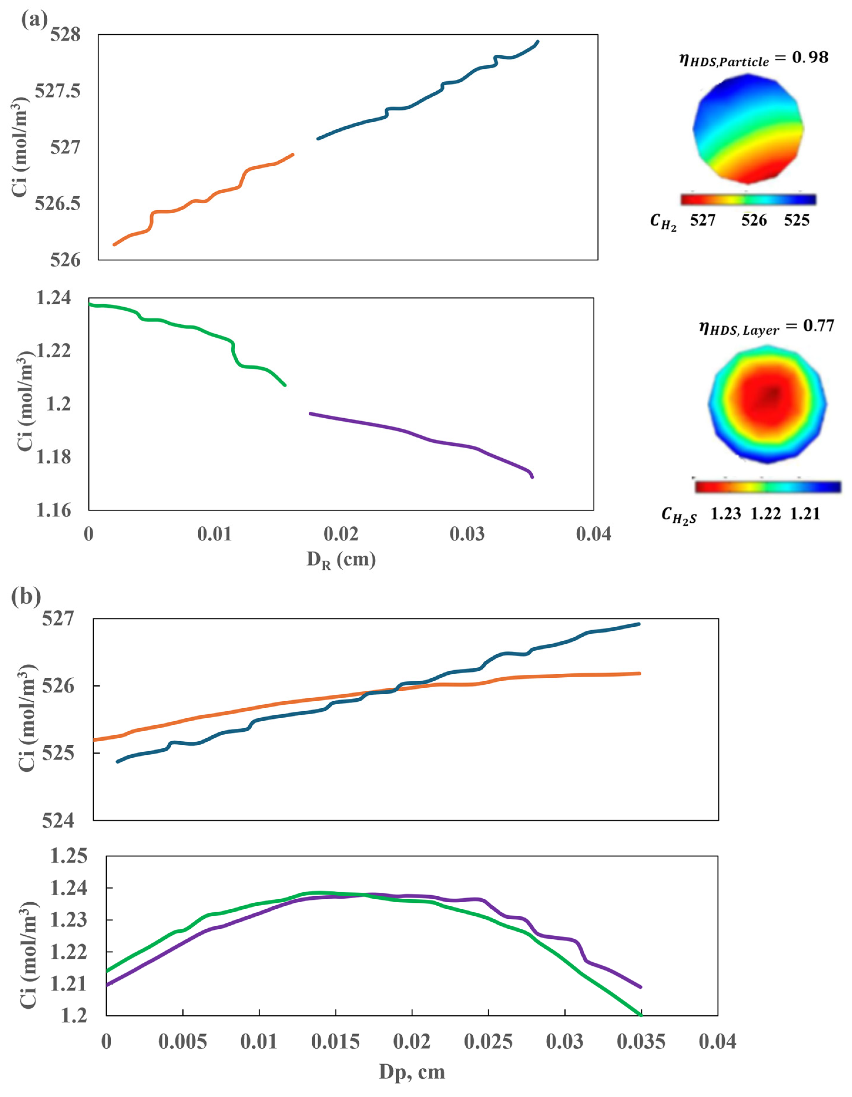
To interpret the global transport phenomena in the RMS model, a comparison is made between the dominant transport mechanisms in different sections of the reactor.
Figure 13a,b and
Figure 14a,b illustrate a plane cut in the axial direction in the reactor’s mid-section, wherein the concentrations and fields of diffusive and convective fluxes are depicted. The first of these is the wall region, in which the channeling of approximately 1-5-2 catalyst diameters is observable. The second is the central region, in which convective transport is found to be insignificant.
The convective transport fluxes for the two reaction species, R-S and H
2S, as illustrated in
Figure 14 and
Figure 15, exhibit a pronounced dominant transport behavior in the axial direction. Additionally, the flux at the walls is observed to be up to 10
5 times higher than at the reactor center. Conversely, the diffusive flux of R-S and H
2S species evidences a discernible transport trend in the radial direction. It is noteworthy that for H
2S, the diffusive flux path vectors represent a countercurrent transport. This is because H
2S is produced within the central region, resulting in concentration gradients that extend from the outlet to the inlet and from the center to the walls. Similarly, the wall effects have a significant influence in regions of the RSM model, as illustrated in
Figure 13 and
Figure 14.
A discontinuity in the H
2S flux is evident in the vicinity of the liquid–solid interface. It should be noted that the proposed model incorporates an additional resistance for the transport of H
2S at the catalyst–liquid interface.
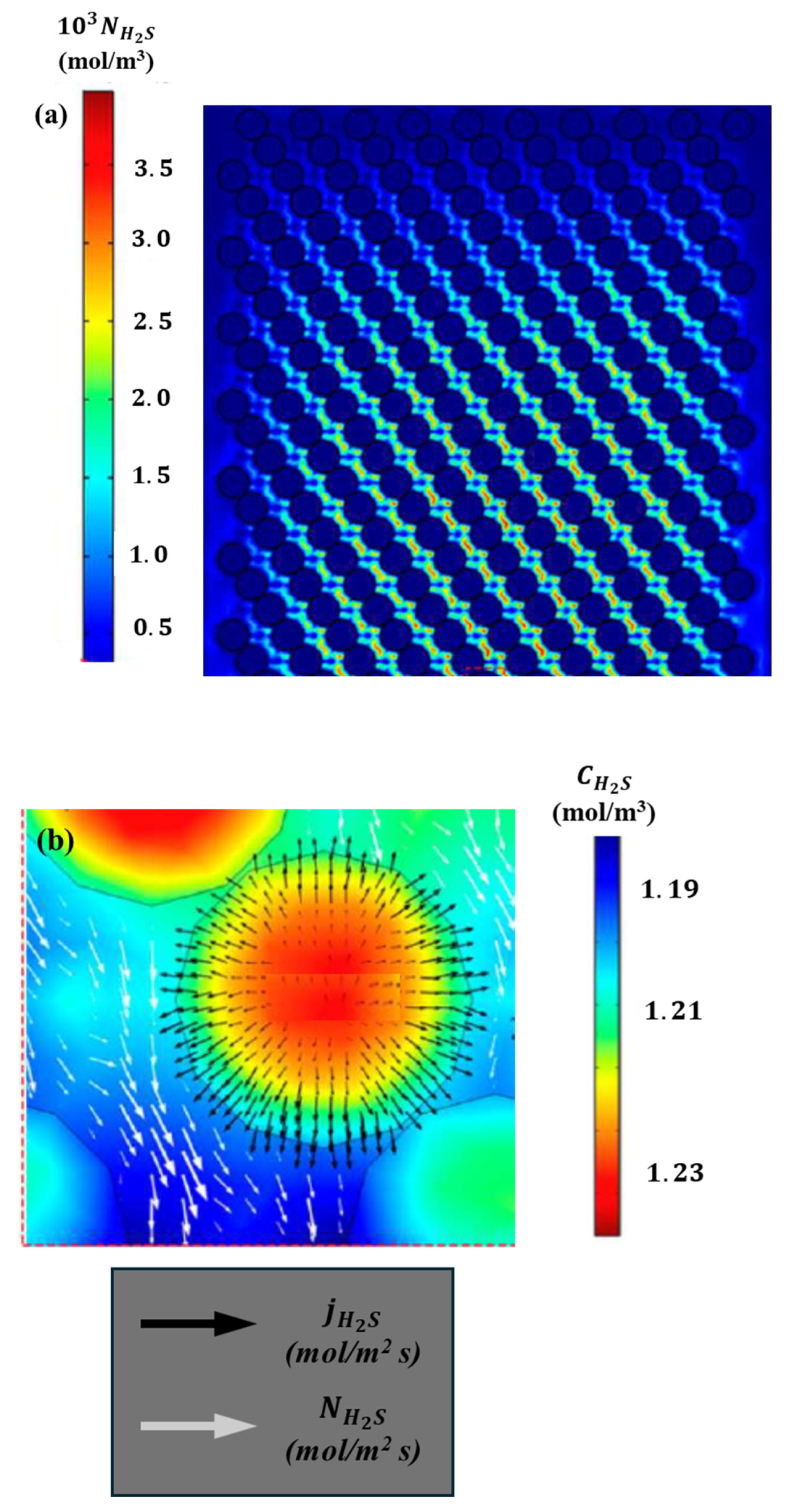
Figure 15b illustrates the detailed profiles, which show a close-up of the H
2S concentration field in the catalyst particle at the central cut-off line of the diameter. The direction of H
2S transport is also indicated by the flux vector arrows in the catalyst particle and the liquid surrounding the particle. As illustrated in
Figure 15b, the total flux of H
2S exhibits significant fluctuations along the radius. The proposed CFD model is analogous to an experimental reactor utilized to ascertain kinetic parameters under a plug flow pattern, which is devoid of radial gradients.
The results presented in
Figure 15b indicate that this assumption may be insufficient and that the kinetic outcomes may be unreliable. The results of the hydrodynamic and kinetic analysis conducted for other chemical species are comparable, which underscores the importance of considering effects in the radial direction. These findings can be validated by examining the concentration fields depicted in
Figure 13 and
Figure 14. At the interface between the liquid and the catalyst surface, the flux field exhibits a discontinuity, which can be attributed to the incorporation of resistance terms associated with the boundary conditions employed. The concentration field for H
2S in both the solid and the surrounding liquid is markedly asymmetrical, exhibiting a considerable range of concentration variability
) given that the diameter of the catalyst particle is 0.35 mm. Furthermore, the remaining chemical species exhibit asymmetries in the fields and substantial variations in the radial and axial coordinates, as illustrated in
Figure 16. The proposed multi-scale model reveals notable discrepancies in the behavior and distribution of concentration fields within the catalytic bed. These differences have a significant impact on the kinetic behavior of the reactor, which is a consequence of the coupling of transport phenomena at different scales.
In a laboratory-scale TBR reactor, Silva et al. [
50] conducted an analysis of the HDT of diesel, including HDS and HDA reactions. To investigate the proposed reactions, a three-dimensional multi-phase Eulerian–Eulerian approximation was developed, taking into account interfacial interaction. Furthermore, a porosity distribution model for trilobular catalyst particles and mass transfer was incorporated into the kinetic model to account for these effects. Considering the relatively modest dimensions of the reactor under examination, the simulation was conducted under the assumption of isothermal and transient conditions, in addition to the full wetting of the catalyst. Two distinct flow configurations were subjected to analysis: countercurrent and co-current. The analysis encompassed the examination of conversion, pressure drop, and liquid holdup, with a particular focus on the changes in pressure, temperature, flow, and velocity of the gas and liquid streams. Additionally, the impact of porosity on fluid velocity and liquid volume fraction was examined. Furthermore, the impact of the velocity–velocity space (LHSV), temperature, gas–liquid ratio, and partial pressure of H
2S was also examined. The kinetic parameters utilized in that study were derived from Gunjal et al. [
43] The outcomes of the CFD model simulations regarding temperature fluctuations are illustrated in
Figure 17a–c. As illustrated in
Figure 17a, the conversion of sulfur compounds is observed to increase with increasing temperature. These findings are in accordance with the experimental results reported by Chowdhury et al. [
45].
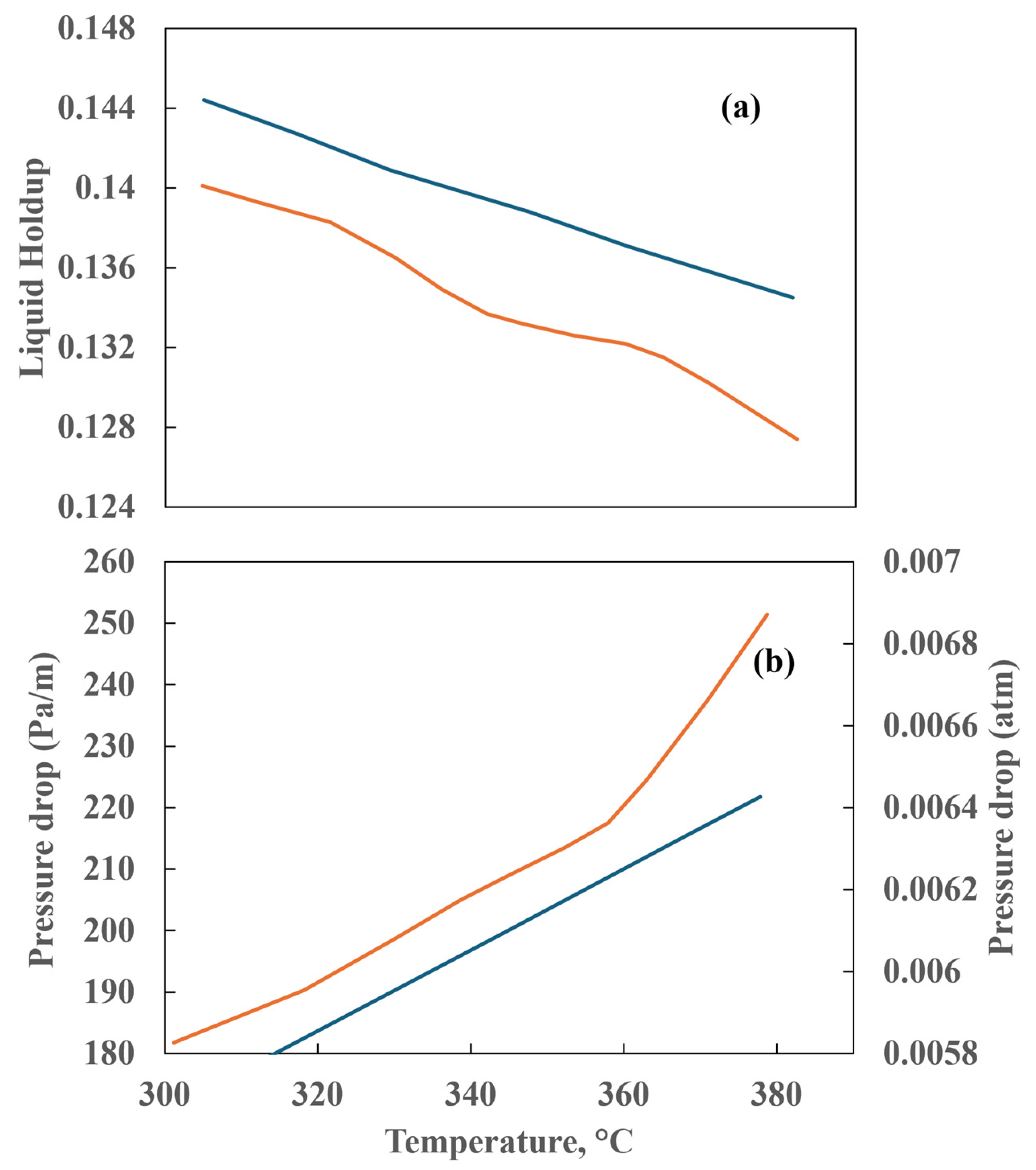
The results of the liquid holdup and pressure drop at varying temperatures are illustrated in
Figure 18a,b.
Figure 18a shows that the countercurrent reactor exhibits a higher liquid holdup than the co-current reactor. Additionally, the data demonstrate an inverse tendency between liquid holdup and temperature. In a countercurrent configuration, in which the two fluids flow in opposite directions, the gas is observed to retain a greater quantity of liquid in the reactor. While the temperature rises, the liquid viscosity diminishes, resulting in an increase in velocity. This leads to a reduction in the accumulation of liquid within the reactor, which is reflected in a lower liquid holdup. Conversely, the pressure drop increases with temperature, as observed in
Figure 18b, due to the liquid’s role as a barrier. As the temperature increases, the density and viscosity of the liquid phase decline, allowing it to occupy a greater volume flowing at higher velocity against the gas phase.
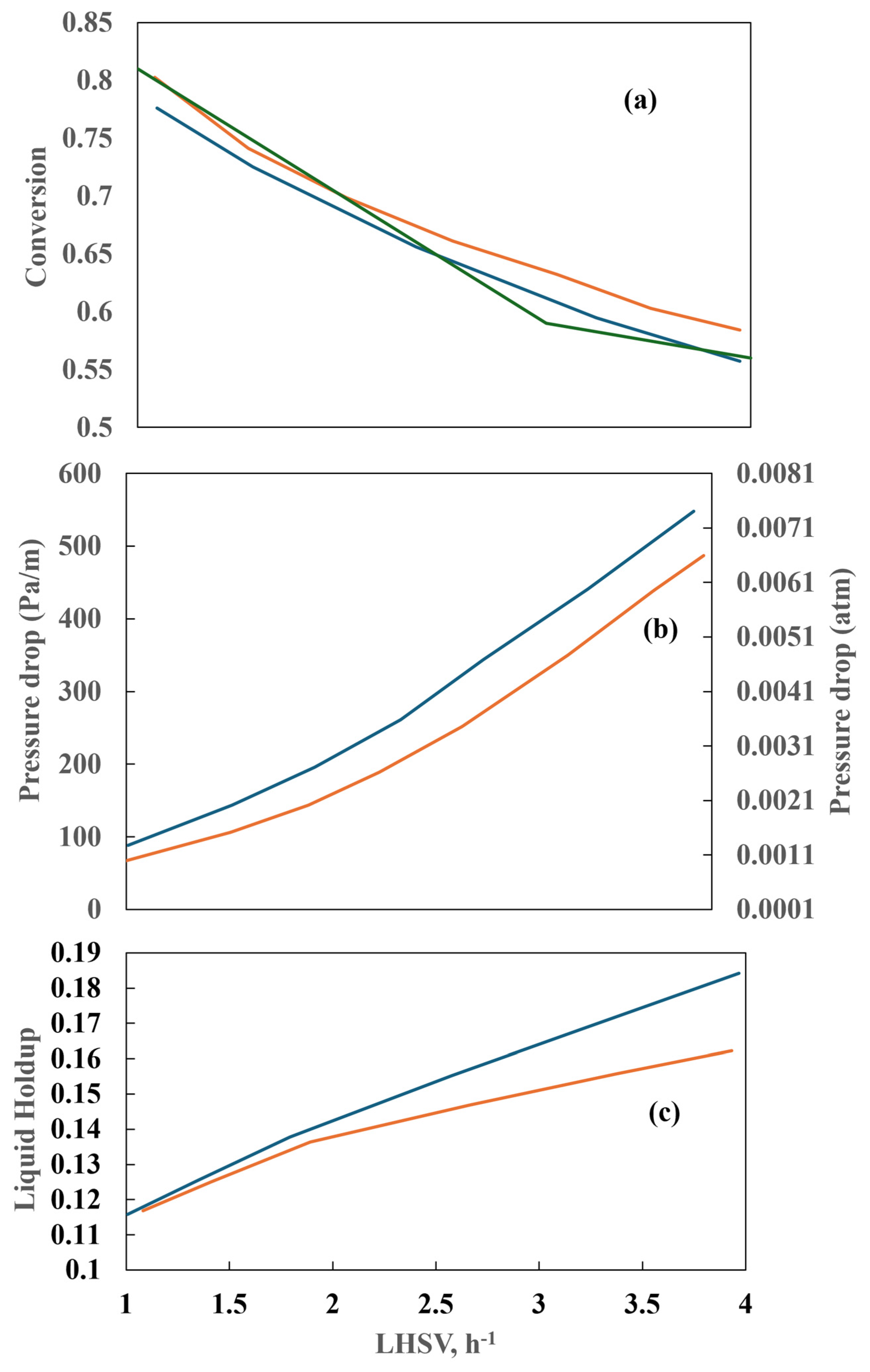
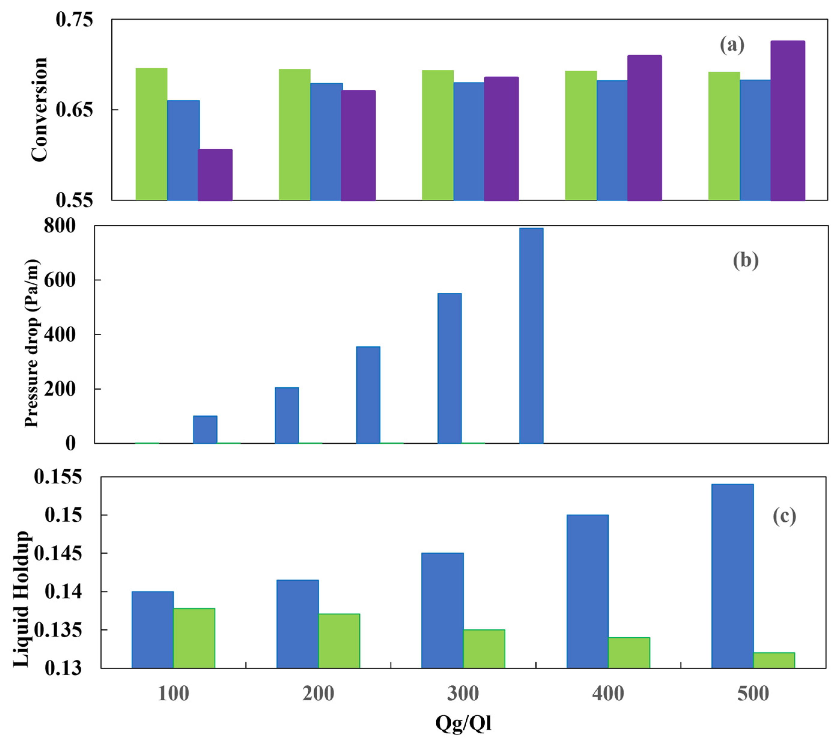
By varying the LHSV while keeping the other parameters at a constant value, the conversion shows an asymptotic behavior, as shown in
Figure 19a. On the other hand, the conversion decreases as the LHSV increases, and the LHSV also influences the pressure drop (
Figure 19b). The pressure drop for bench reactors is commonly neglected. For a low liquid diesel flow, the pressure drop is identical for both the countercurrent and co-current flows, but it differs at high liquid flows. The higher-pressure drop in the countercurrent reactor is explained by the fact that both phases flowing in opposite directions have greater interaction.
Figure 20a depicts the conversion achieved in the two reactors when the gas–liquid flow ratio is varied and shows that the gas–liquid flow ratio exerts no influence on sulfur conversion. However, in the experimental and industrial runs, the dependence of sulfur conversion on the gas–liquid flow ratio is more pronounced than the simulated values. The higher the gas–liquid flow ratio, the higher the pressure drop.
Figure 20b shows the influence of the counterflow arrangement on the pressure drop.
Figure 20c illustrates the liquid holdup for both the countercurrent and co-current schemes. It is noteworthy that the countercurrent configuration yields a higher liquid holdup for a given gas–liquid flow ratio, which is attributed to the drag force that the gas stream exerts on the liquid stream. The sulfur conversion is shown in
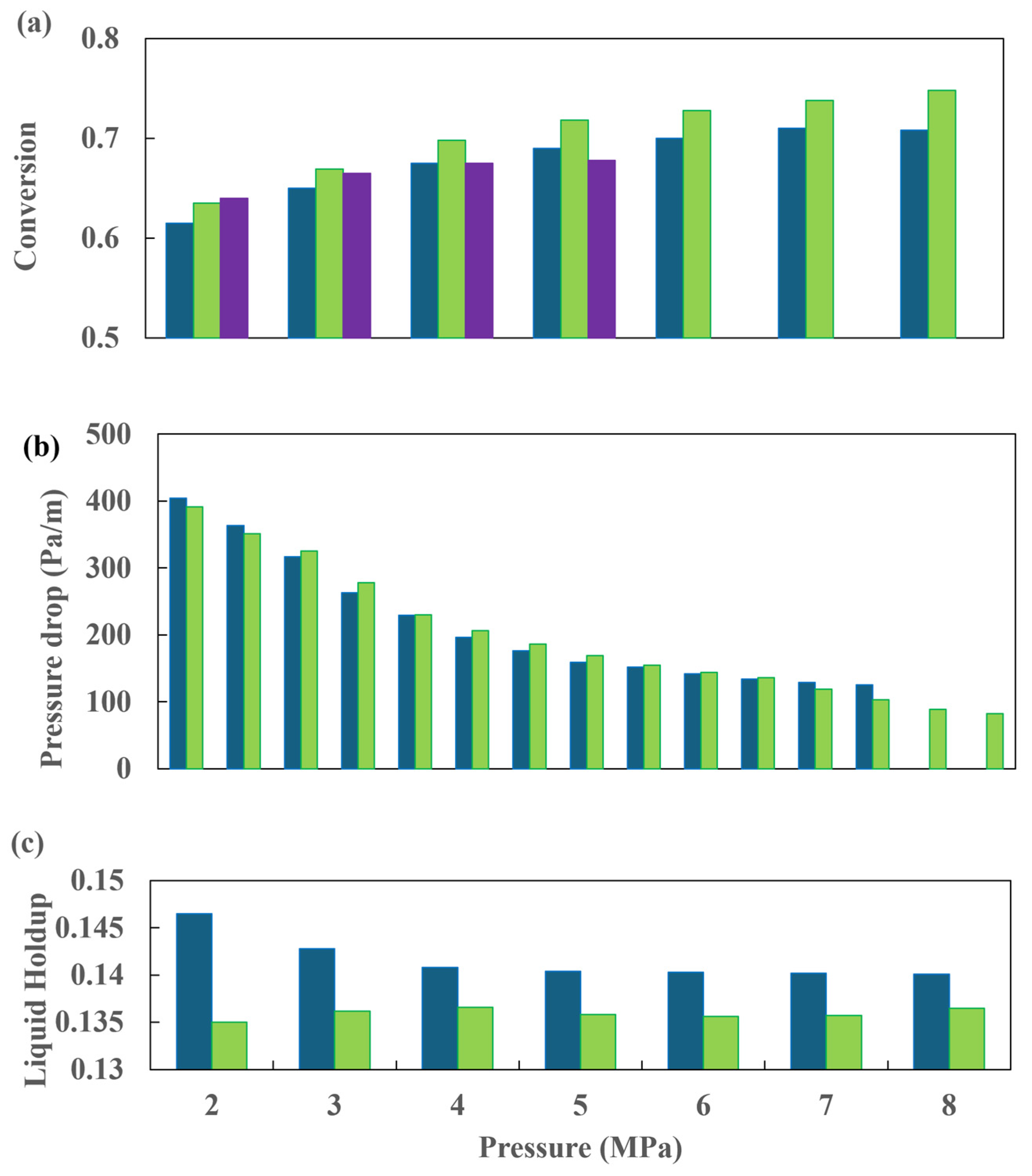
Figure 21a. In general, the CFD simulation results for the two reactor configurations agree well with the experimental data. An increase in pressure increases the transfer of hydrogen present in the gas to the liquid, and consequently, the sulfur conversion is improved.
The CFD simulations indicate that when the operating pressure is increased, the co-current arrangement exhibits a slightly higher conversion rate than the countercurrent flow.
Figure 21b shows the pressure drop behavior with respect to the operating pressure. The liquid holdup profile is presented in
Figure 21, and it is observed that the influence of the total pressure is negligible in comparison to the other variables. The outcomes yielded by both flow configurations are comparable, although the countercurrent configuration results in lower conversion rates. Silva et al. [
50] presented one of the most comprehensive investigations conducted to date. It can be considered an exemplary reference for those engaged in the development of a partial or comprehensive study of a diesel HDT reactor.
The diffuser in a HDT reactor is designed to eliminate turbulence in the feed stream, while the distributor plate is responsible for establishing a uniform gas–liquid flow pattern as the fluid enters the catalytic bed. This configuration facilitates optimal catalyst wetting, thereby enhancing the efficiency of catalyst utilization. The current state of research in this field is deficient in simulations of the diffuser. Furthermore, investigations related to the distributor plate through CFD remain scarce. Some of the related research with CFD simulation is presented in this article.
Subramanian et al. [
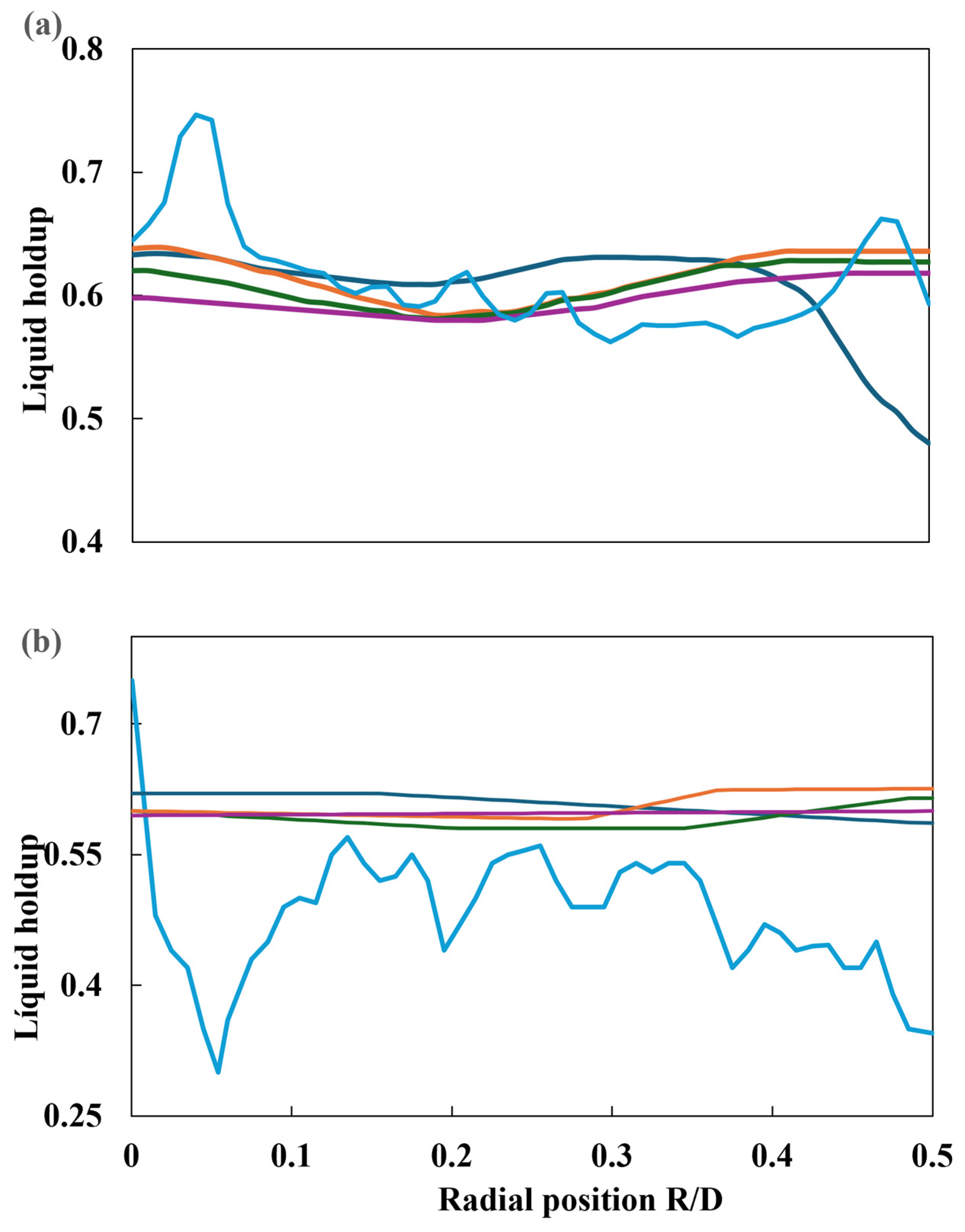
47] proposed a Eulerian–Eulerian CFD model for simulating gas–liquid co-current flow through a solid foam bed, with the objective of mimicking the packed bed of the TBR. Subsequently, the gas–liquid phase was conveyed through the distributor plate, whereupon the flow wetted the catalytic bed. The distributor plate was modeled in two distinct ways. The first was as a single orifice for liquid flow, with a diameter of 5 mm. However, it is unclear if both phases crossed this perforation. The second was as a plate with multiple orifices, comprising twelve perforations with a diameter of 4 mm for the liquid phase, while the gas flowed through four orifices with a diameter of 9 mm. The results are summarized in
Table 6. Following the validation of the model with experimental data, a series of simulations were conducted to assess the gas and liquid surface velocities, the impact of the packed bed on liquid retention, and the pressure drop of liquid and gas phases due to capillary and mechanical forces for both distributor plate types. The CFD model reproduced the liquid holdup and two-phase pressure drop obtained from experimental runs, using foam as packing (20 and 30 pores per inch). For each type of packing, two surface velocities of gas and liquid were used to obtain a comprehensive understanding of the phenomenon under investigation. Liquid retention in the radial direction was conducted at two distinct elevations. The measurements were taken from the top inlet at two heights: 0.25 m (L/D = 2.5) and 0.65 m (L/D = 0.65). A comparison of the radial profiles for different flow conditions is presented below. In each case, four simulations are developed, considering the following scenarios: (i) no dispersion forces, (ii) capillary forces, (iii) mechanical forces, and (iv) mechanical and capillary forces. Different liquid holdup values (L/D = 2.5 and L/D = 6.5) are plotted in
Figure 22.
The influence of dispersion forces on liquid retention is observed to be minimal. To further analyze the impact of dispersion forces on liquid retention, additional runs were conducted in the vicinity of the reactor inlet at L/D = 0.1 and L/D = 0.5. The results obtained are presented in
Figure 23. The initial profiles exhibit a pronounced disparity when the simulations that consider dispersion forces are compared to those that do not. In the absence of dispersion forces, the liquid holdup attains a maximum value below the liquid inlet holes, while in the region proximate to the walls, no liquid is present. The results obtained at these locations demonstrate that at L/D = 0.1, there is a notable increase in the liquid holdup towards the center of the reactor, accompanied by a considerable decrease towards the walls. Conversely, at L/D = 0.5, the liquid holdup exhibits a profile similar to that observed downstream, displaying minimal variation and a slight decrease towards the walls.
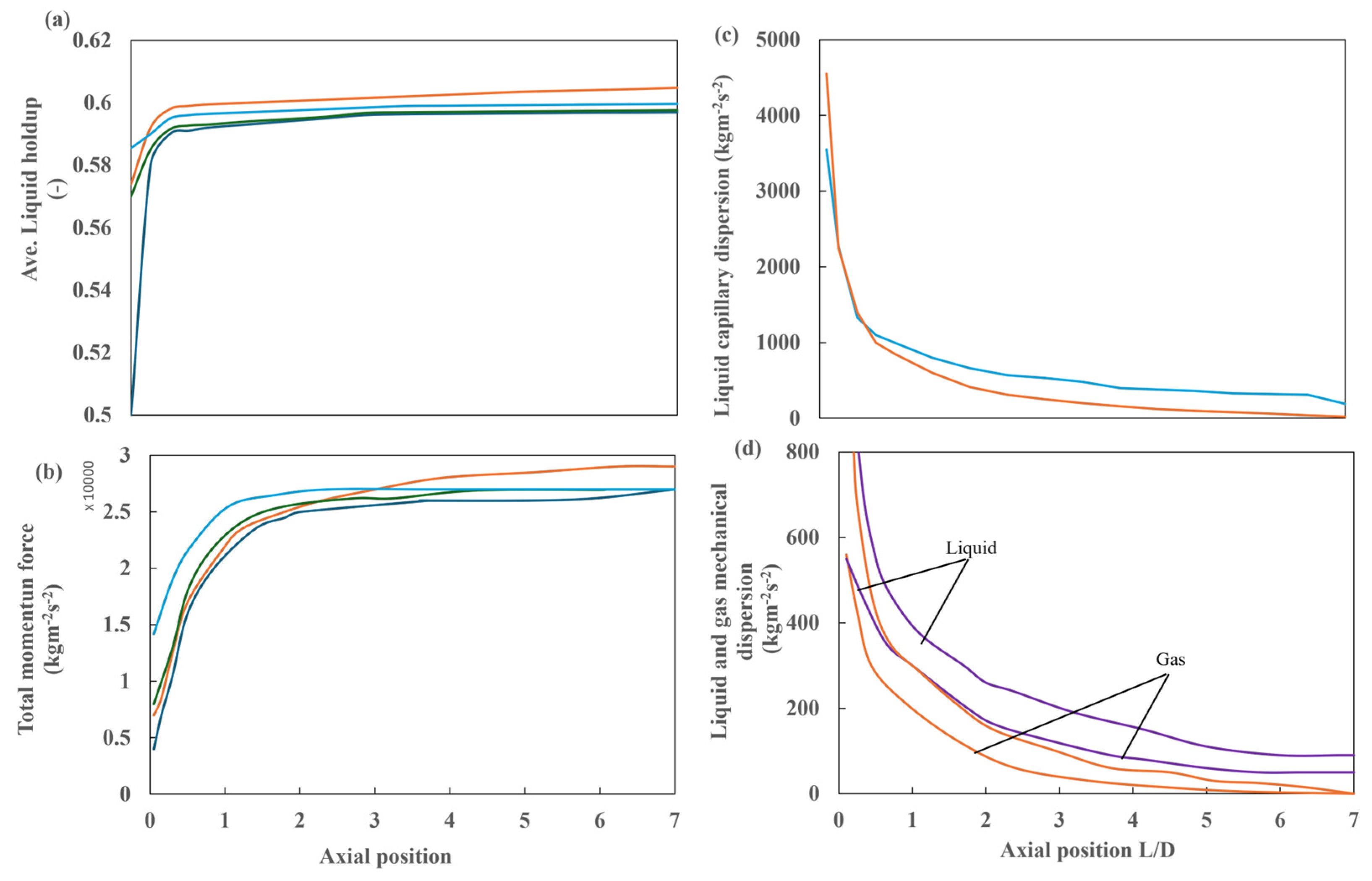
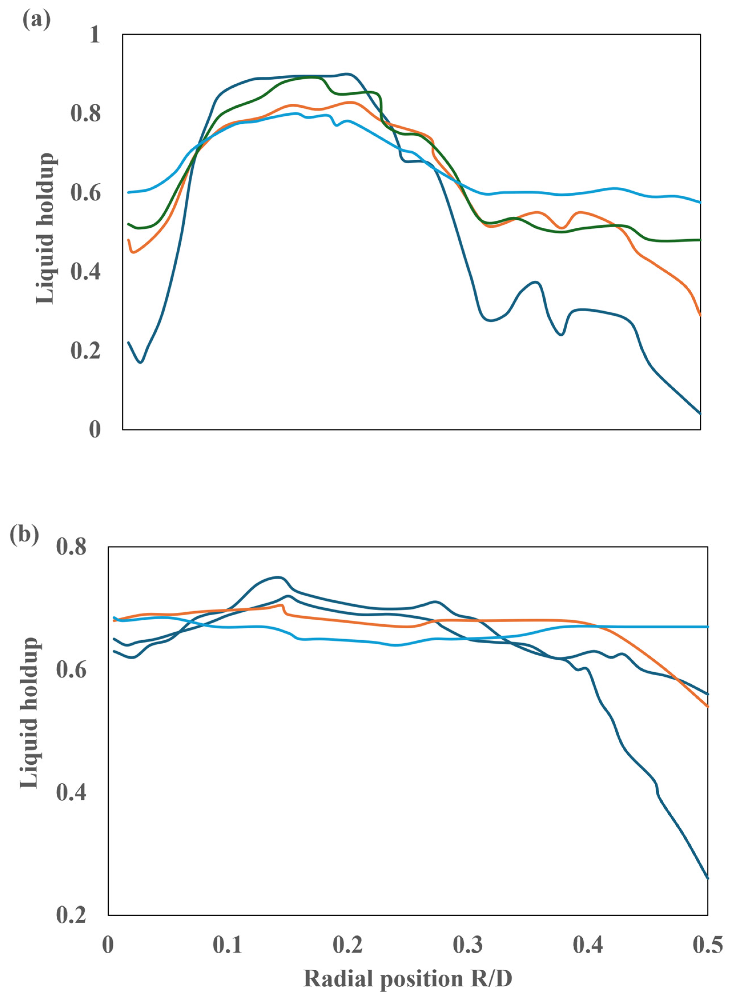
Figure 24 shows the detailed analysis of liquid retention, total momentum, and capillary and mechanical dispersions of gas and liquid for case 4.
Figure 24a shows the average liquid retention, which increases exponentially near the inlet to a constant value at L/D = 1.
Figure 24b illustrates that the total momentum with respect to the reactor length also increases exponentially, reaching a constant value at approximately L/D = 2. At this point, the total momentum reaches a value of approximately 26,000 kg m
−2 s
−2. The same trend is observed in the other simulation cases, with no change in the dispersion forces. This is similarly evident in the behavior of liquid capillary dispersion and capillary and mechanical dispersions of gas and liquid, which demonstrate an exponential decrease up to the same inflection points, i.e., L/D = 1 and L/D = 2, respectively. The capillary dispersion values are notably elevated in the vicinity of the inlet, reaching a maximum value of 300 kg m
−2 s
−2 at L/D = 2.5. This value then decreases to 40 kg m
−2 s
−2 at L/D = 6.5.
Subramanian et al. [
47] also analyzed the effect of phase flows and packing porosity, as well as the effect of pressure drop on fluid retention, and all the results presented up to this point correspond to simulation cases using a multipoint distributor. Similarly, Subramanian et al. [
47] presented a summary of results obtained using a single-point distributor. Finally, a comparison was made with the simulation of a TBR reactor. Their conclusions indicate that the impact of mechanical and capillary dispersion forces is more pronounced in the vicinity of the reactor inlet. If dispersion forces are disregarded, a diminished impact of liquid retention near the walls is anticipated. The incorporation of dispersion forces results in a more uniform distribution of the liquid in the vicinity of the inlet. The impact of the dispersion could not be discerned in the downstream region beyond the reactor for the multipoint distributor. The multipoint distributor serves to counteract the influence of dispersion forces, and thus, their influence cannot be observed beyond a certain height of the reactor. Overall, the mechanical and capillary dispersions contribute 1 to 2% of the total momentum force. Additionally, it was observed that both types of dispersions exhibited an exponential decrease along the reactor in the flow direction.
When a multipoint distributor is used, a uniform liquid distribution is observed at different reactor heights, which has been also reported in studies on a TBR reactor. However, simulations considering a single-point distributor show significant changes in liquid retention when dispersion forces are considered. On the other hand, the trend of mechanical and capillary dispersions for a single-point distributor is also different as it increases exponentially along the reactor in the flow direction. It can be concluded that the developed model accurately predicts the average liquid retention near the outlet, at a height of 0.65 m. However, the model demonstrates a lack of precision in its predictions near the entrance, at a height of 0.25 m.
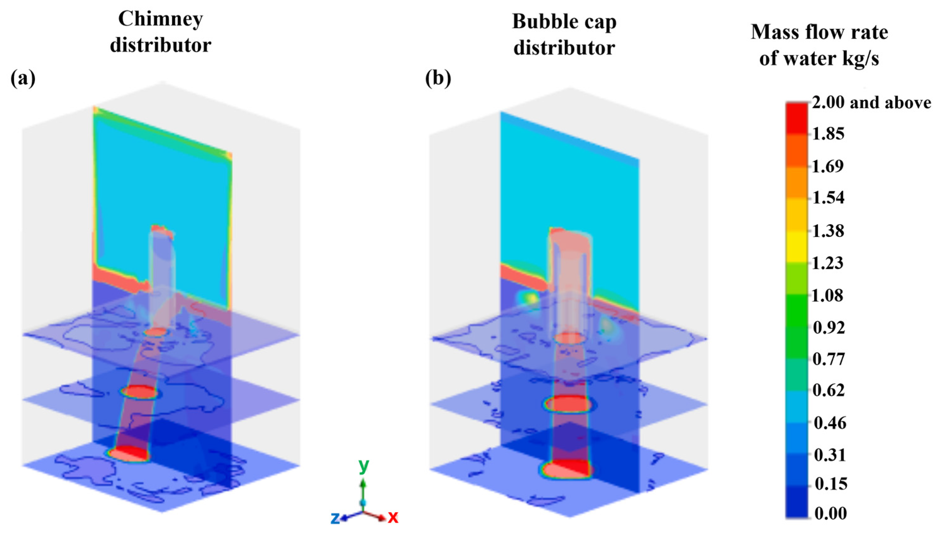
Jain et al. [
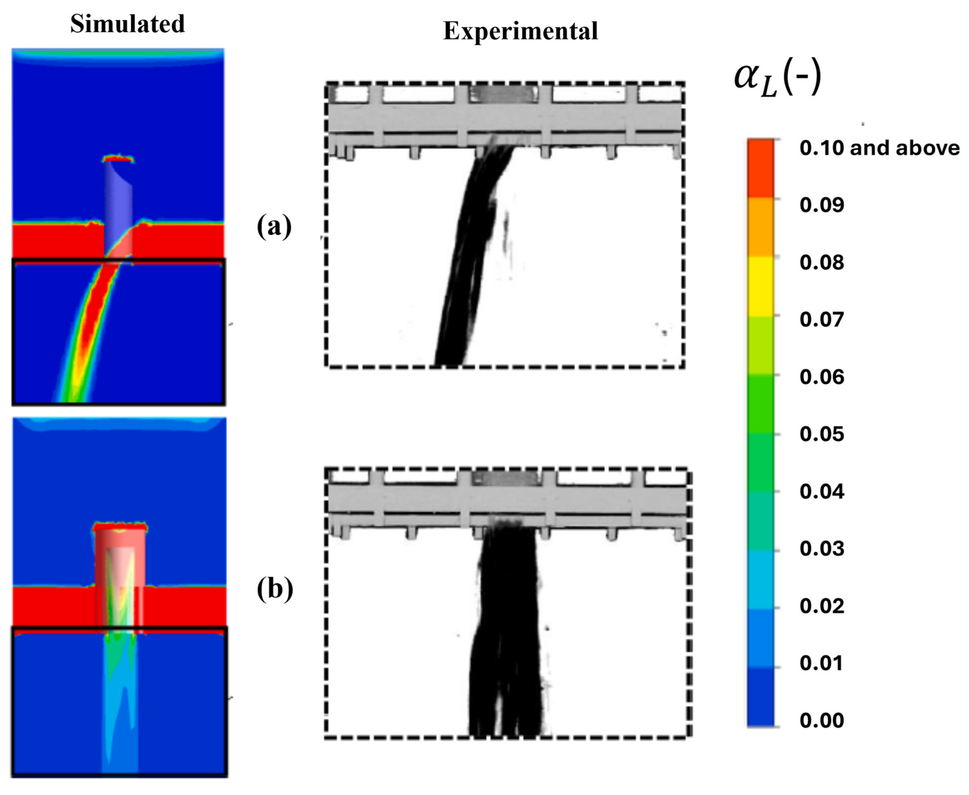
51] conducted a study of a chimney distributor element as well as a bubbling cap distributor element. The distributor plates are the most important devices for achieving the most optimal distribution of the gas–liquid mixture over the catalytic bed. In this study, the researchers employed a CFD model based on a two-fluid Eulerian approximation to simulate the flow of the gas–liquid mixture in the diverse regimes present throughout the distribution elements. The results were validated against the liquid distribution measured using high-velocity imaging, the gas–liquid flow morphology measured with vacuum probes, and the pressure drop. The results obtained revealed a significant difference in the flow patterns observed in the chimney and bubble cap distributor elements. This finding led to the conclusion that the liquid discharge patterns, the uniformity and symmetry of the flow streams, and the pressure drop across the distributor plates are significantly different. Moreover, it has been demonstrated that the incorporation of an additional distribution stage at the outlet of the primary distribution element enhances the liquid distribution pattern by encompassing a broader range and a more dispersed gas–liquid stream. This study demonstrated the predictability of the distribution of gas–liquid mixing across industrial plates, employing both bubble cap plates and chimney plates for the purpose of examining the distribution of liquid generated in a co-current downflow configuration using air and water as a gas–liquid mixture.
Figure 25 shows the acquired and experimentally processed images and numerical predictions of the average liquid distributions flowing through the chimney manifold and the bubbling cap manifold. The numerical model predictions are in good agreement with the processed images of the flow through both distributors.
Figure 26 illustrates the distribution of liquid mass flow through the distributors. In both cases, the liquid stream coverage range is observed to increase as a function of distance from the distributor element. However, the wetted area was found to be only 10.6% and 16.0% for the chimney and bubbling cap, respectively. This suggests that a significant portion of the industrial-scale catalyst would remain in a dry state in the absence of optimized distributor plate configuration.
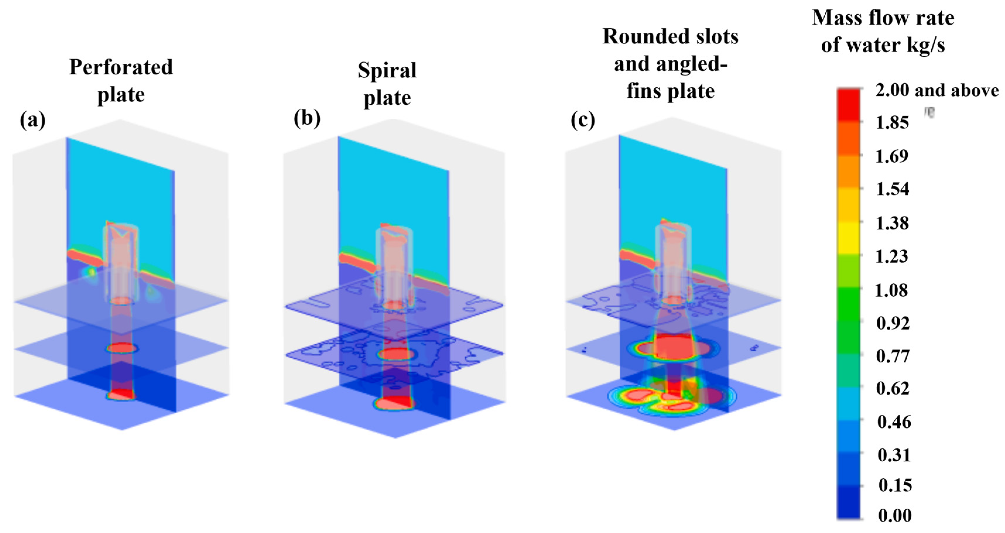
Figure 27 illustrates the distribution of the liquid generated by the bubbling cap with two types of post-distribution: a perforated plate and a spiral plate. The experimental measurements are presented on the right, while the predictions are shown on the left of the average liquid distribution. It can be observed that there is a reasonable degree of agreement between the two sets of data. The figure also shows the time-averaged mass flow rate of the liquid distribution on the
y-axis (kg/s) flowing through a post-distribution stage unit for (a) a perforated plate, (b) a spiral plate, and (c) a plate with rounded openings and inclined fins.
It is observed that in both
Figure 26a and
Figure 27a, the liquid coverage interval generated by the bubble hood with the redistributor plate is narrower than that obtained in the absence of the redistributor plate. Nevertheless, although the incorporation of the redistributor plate does not lead to an expansion of the liquid distribution coverage interval in the outlet plane, it does enhance the homogeneity of the liquid distribution.
As evidenced by the research works cited above, the application of CFD is highly versatile for the hydrodynamic simulation of the HDT process. It can be employed to simulate a range of phenomena, including the flow in the inlet pipe, the flow through the diffuser, and the flow through the main distributor plate. Additionally, it can be used to simulate the flow of the gas–liquid mixture through the catalyst-packed bed, including or excluding the impact of the flow on the chemical reactions.
Nevertheless, the analysis of the literature indicates that investigations employing CFD simulation for all sections of the HDT reactor remain limited. This is partly due to the fact that the CFD computational tool has not yet been widely adopted for the analysis of petroleum refining processes, despite significant advances in its capabilities over the past decades. Additionally, the complexity of implementing CFD simulations and the scarcity of CFD specialists capable of performing such analyses have contributed to the limited utilization of this technique.


 ,
, 


 ) Experimental, (
 ) 0.05 m, (
 ) 0.65 m, (
 ) 1.28 m, and (
 ) center.

 ) Commercial scale: Total Ar. (
 ) Laboratory scale: Total Ar [46].

 ) Poly-Ar Lab, (
 ) Di-Ar Lab, (
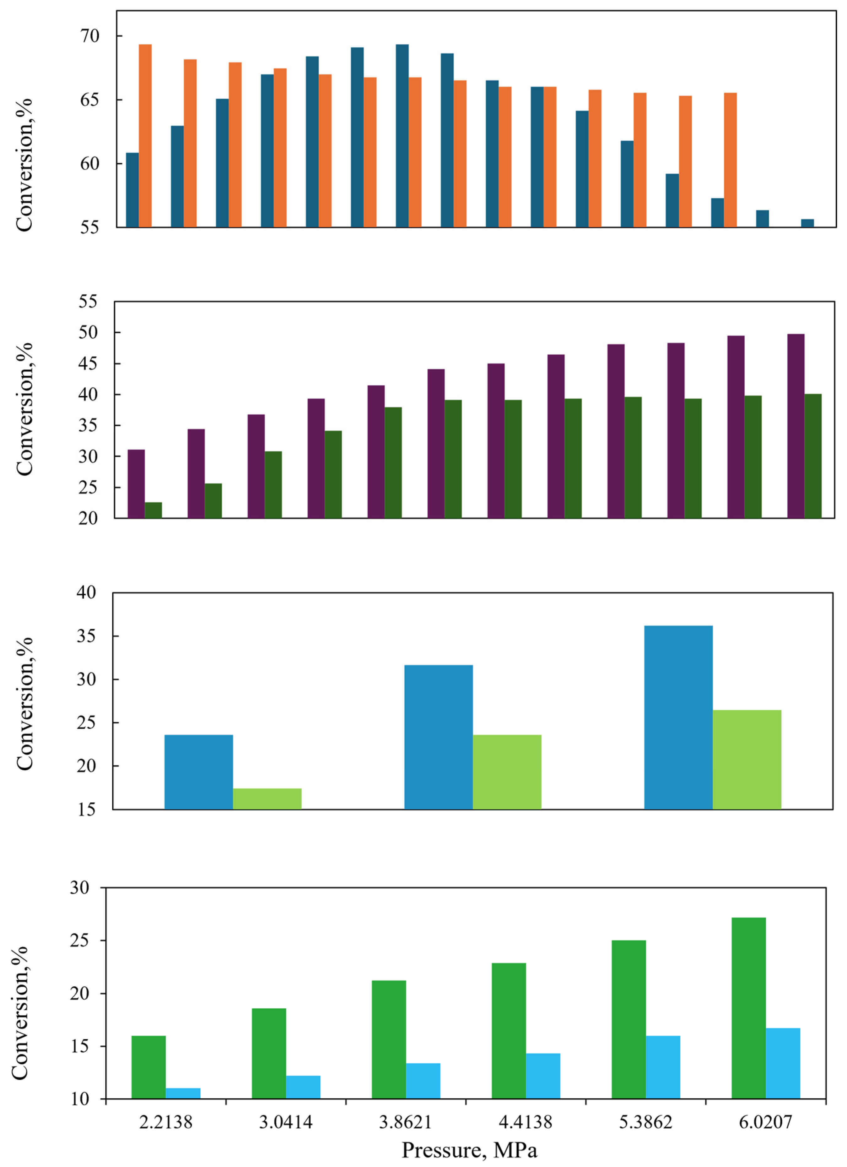
 ) Poly-Ar Commercial, (
 ) Total Ar Commercial, and (
 ) Total Ar Lab.
 ) Mono-co-current, (
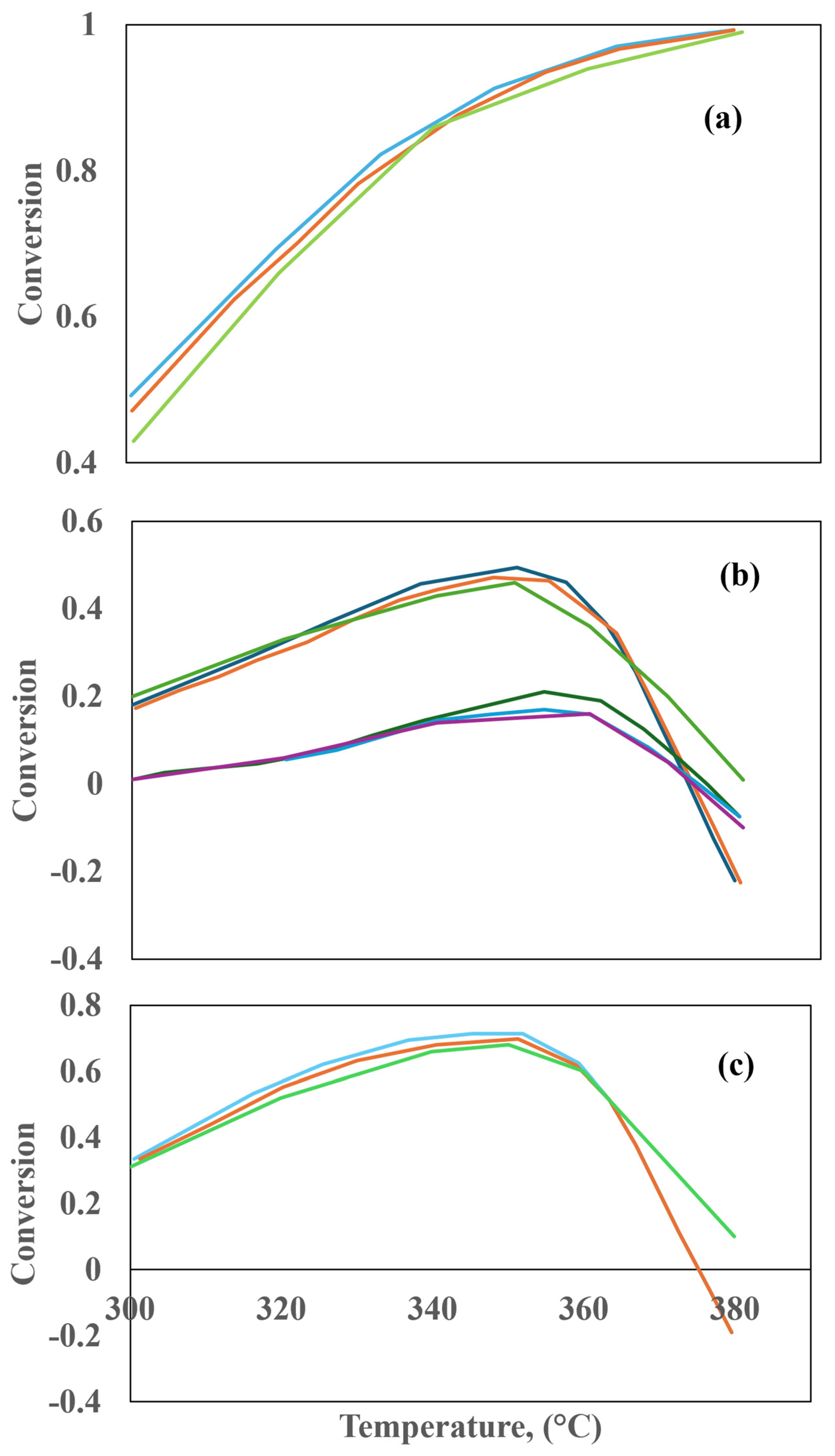
 ) Experimental [50].
 ) Capillary only, (