Abstract
The automatic detection of objects in medical photographs is an essential component of the diagnostic procedure. The issue of early-stage brain tumor detection has progressed significantly with the use of deep learning algorithms (DLA), particularly convolutional neural networks (CNN). The issue lies in the fact that these algorithms necessitate a training phase involving a large database over several hundred images, which can be time-consuming and require complex computational infrastructure. This study aimed to comprehensively evaluate a proposed method, which relies on an active contour algorithm, for identifying and distinguishing brain tumors in magnetic resonance images. We tested the proposed algorithm using 50 brain images, specifically focusing on glioma tumors, while 2000 images were used for DLA from the BRATS Challenges 2021. The proposed segmentation method is made up of an active contour algorithm, an anisotropic diffusion filter for pre-processing, active contour segmentation (Chan-Vese), and morphologic operations for segmentation refinement. We evaluated its performance using various metrics, such as accuracy, precision, sensitivity, specificity, Jaccard index, Dice index, and Hausdorff distance. The proposed method provided an average of the first six performance metrics of 0.96, which is higher than most classical image segmentation methods and was comparable to the deep learning methods, which have an average performance score of 0.98. These results indicate its ability to detect brain tumors accurately and rapidly. The results section provided both numerical and visual insights into the similarity between segmented and ground truth tumor areas. The findings of this study highlighted the potential of computer-based methods in improving brain tumor identification using magnetic resonance imaging. Future work must validate the efficacy of these segmentation approaches across different brain tumor categories and improve computing efficiency to integrate the technology into clinical processes.
1. Introduction
A tumor is an abnormal tissue mass that grows uncontrollably, resulting in serious health problems [1]. Brain tumors are abnormal cell growths in the cranial cavity, either cancerous or benign. Their distinct, symmetrical structure and absence of actively dividing cells can identify them [2]. Accurate neuroimaging techniques are crucial for early identification of brain cancer and associated structures and enabling timely chemotherapy administration. In [3], the authors classify brain tumors as benign (non-cancerous) or malignant (cancerous) based on variables such as the tumor’s origin, development pattern, and carcinogenic qualities. Although benign tumors are non-cancerous and easily removed, they may exert pressure on sensitive brain areas. Conversely, malignant tumors have an irregular appearance and active cell division, develop quickly, and penetrate healthy brain tissue. Notably, not all malignant tumors invade healthy tissues. However, medical imaging is crucial in identifying, diagnosing, and treating brain tumors. Recognizing a brain tumor involves a comprehensive neurological evaluation, brain imaging scans, and, in some cases, an analysis of brain tissues [4]. Among various imaging techniques, magnetic resonance imaging is the most preferred method. Magnetic resonance imaging (MRI) is a high-tech medical imaging tool that gives detailed information about the structure of soft tissues in the human body. The medical imaging domain primarily utilizes MRI to comprehensively analyze the anatomical structure and physiological functioning of the human body. MRI is a complex medical imaging technique that produces high-quality images of the human body. People widely use it to assess brain tumors [5]. MRI high-resolution images give precise anatomical details that aid in evaluating brain development and identifying structural variations [6,7,8].
The advancement of MRI technology in the field of neuroimaging has provided progressively significant insights into the functioning of the human brain [8]. However, healthcare practitioners have faced significant challenges in processing MRI data due to the labor-intensive and error-prone method of extracting crucial data from intricate and extensive MRI datasets. The process of manual analysis is prone to errors. It is also time-consuming, particularly due to the presence of multiple inter- and intra-operative variances that are inherent in MRI examinations. Hence, it is imperative to develop computer-based approaches that are more efficient in the automated detection and diagnosis of medical issues utilizing MRI data [9,10]. MRI employs segmentation techniques to distinguish between regions of potential brain tumors and normal cerebral tissue [11]. These techniques encompass a variety of methods, including area-based, edge-based, cluster-based, super-pixels-based, fusion-based, hybrid, and optimization-driven segmentation, among others [12]. Diagnosing a brain tumor is difficult, nevertheless, because of the several features of brain tumor appearances in photographs that differ in edges, shapes, and textural qualities. These features complicate diagnosis of brain malignancies [13,14].
Particularly with the integration of semi-automatic approaches that mix clever algorithms with human skill, the identification of brain cancers using MRI images has considerably advanced. Moreover, human factors subject a radiologist’s traditional manual examination of MRI scans to validity issues, making it time-consuming [15]. Researchers are addressing these challenges by exploring semi-automatic approaches that aim to enhance the efficiency and consistency of early tumor detection. A key part of semi-automatic detection systems is using machine learning to process images. Studies have focused on basic image processing methods like thresholding, region growing, and edge detection for finding abnormal areas in MRI scans [16]. These techniques typically lack the complexity to differentiate between numerous forms of brain tissues and the dependability of malignancies. Tumor identification uses automatic methods including K-means and fuzzy C-means and intensity-based segmentation.
Three primary phases comprise the detection process; in the early phase, it employs preprocessing methods to eliminate noise and distortion from the set of MRI images. In the next phase, the segmentation technique detects the tumor in the brain scans by means of preprocessed images. Several documented techniques exist for different areas of an MRI brain scan [17].
Furthermore, a study conducted by [18] compared three distinct approaches: Otsu thresholding [19], K-means, and fuzzy c-means (FCM). They use these methods to extract tumors from a total of 25 MRIs [20]. The assessment encompassed an analysis of both the precision of the extraction process and the time required. The fuzzy-c-means approach exhibited the highest level of accuracy, obtaining a notable accuracy rate of 90.57% based on the provided data. Additionally, the Otsu holding approach required a shorter computation time, but its accuracy was lower. In another study, Tripathi et al. (2021) combined Otsu thresholding and K-means clustering methodologies. They assessed the approach on three types of tumor samples from the BRATS 2013 database [21]. They specifically developed the process to differentiate between different tumor elements, including necrotic and edematous areas. They evaluated the accuracy of the method by comparing its outcomes with the ground truth data from the database. They then calculated the Dice coefficient for the three tumor types [21].
In 2022, Babu et al. did a study to see how well different active contour segmentation techniques, like the “Level Set” and “Chan-Vese” methods, worked at finding and locating brain tumors [22]. Furthermore, the researchers sought to assess the performance of the determined brain tumor segmentation approach through a comparative analysis. They used the methodologies to identify brain tumor images within 120 T1-weighted MRI datasets. However, this study selected a limited number of high-quality photos for assessment [22]. According to the results, the “Chan-Vese” algorithm demonstrated higher accuracy than the “Level Set” method in effectively identifying tumors within the selected datasets.
Researchers recently developed several AI algorithms based on machine learning (ML) and deep learning (DL). Sheela et al. 2020 looked at a suggested segmentation strategy along with different methods from different sources, such as progressive deep neural networks and multi-level thresholding. The suggested segmentation algorithm has several important steps that involve using morphological processing techniques to get rid of non-tumor areas. The proposed method also includes a thresholding procedure, the establishment of a circular area encompassing the tumor location, and the use of an initial contour for the Active Contour model. Additionally, the tumor shape dynamically modulates the size of the circular zone [23]. In another study, Sheela et al. 2022 [24] introduced a system that demonstrates efficiency in effectively separating brain tumors. This method utilizes the greedy snake model and fuzzy C-means optimization. By cutting out non-tumor tissue and using morphological restoration techniques, this segmentation method effectively finds the clearly defined region of interest (ROI). In the next stages, encompassing the greedy snake model and fuzzy C-means optimization, the reconstructed image undergoes a threshold process to produce a mask. This mask is subsequently modified to improve the segmentation accuracy [24].
Recently, Aleid et al. proposed a method based on harmonic search optimization for the classification of brain tumors [25]. This method is based on multi-level threshold techniques for tumor segmentation and detection. The method yielded competitive results when compared to state-of-the-art techniques.
Medical image analysis has evolved with machine learning—especially deep learning. CNNs have shown remarkable ability to identify and categorize brain cancers using MRI images.
Despite the advancements, this fully automated system remains imperfect and requires significant computation time and memory [26]. The system has achieved balance by utilizing automated tools for initial detection followed by a radiologist’s review and validation.
Using two distinct pre-trained DL models, a recent DL method [13,27] extracts features from images as vectors. A hybrid feature vector results from combining the vectors under the partial least squares (PLS) method. Top tumor sites are then revealed via agglomerative clustering. Though they require time, their methods have remarkable accuracy.
Recently, an improved UNet method was presented [13], where the results obtained on brain segmentation are about 85% of the average Dice index. With great practical relevance, a recent work in [28] presented a hyperparametric CNN model for brain tumor detection. The aim is to maximize feature extraction and methodically lower model complexity by hyperparameter fine-tuning in the CNN model, thus increasing the accuracy of brain tumor diagnosis.
The key hyperparameters for the model are batch size, layer counts, learning rate, activation functions, pooling techniques, padding, and filter volume. The hyperparameters-optimized CNN model underwent training using three distinct brain MRI datasets accessible on Kaggle. The model achieved notable performance metrics with an average accuracy, precision, recall, and F1 score of 97% and 96% for Dataset1 and Dataset3 respectively. Results varied between 0.91 and 95 on Dataset2.
This work proposes an active contour approach method. The method starts with anisotropic diffusion in the preprocessing step, and the radius contraction and expansion technique [23] is used to get an idea of the border curve around the object of interest. We then used an active contour algorithm, “Chen-Vese,” for segmentation. Finally, we used a post-processing step to refine the segmentation. The results of the proposed method were compared to some of the well-known AI methods using several performance metrics for measurement.
2. Materials and Methods
2.1. Materials
We used 50 brain images from the Brain Tumor Segmentation Challenge BraTS 2021 datasets to test the proposed method (https://www.kaggle.com/datasets/dschettler8845/brats-2021-task1 (accessed on 13 January 2022). For deep learning models, a total of 2000 images were reviewed; 75% (1500 images) were used for training, 20% (400 images) were used for validation, and 3% (50 images) were used for testing. These images originated from multi-parametric MRI (pmMRI) studies focusing on glioma tumors within the same patients. All images in the dataset possessed dimensions of 240 rows and 240 columns [29,30,31]. We conducted our experiments using images previously utilized by other researchers participating in the challenge. This allowed us to compare our findings with those of other methods. Field experts manually segmented each image using the same annotation technique; later, educated neuro-radiologists checked and approved the comments. Three labels—1, 2, and 4—help to classify the images into tumor kinds. La-bel-1 detects label-2 GD-enhancing tumors (ET), label-3 peritumoral edema, necrotic and non-enhancing tumor cores (NCR/NET). After these processes, we resample the BraTS MRI scans to a consistent isotropic resolution of 1 mm 3, co-register them to the same anatomical template (SRI24), and strip the skull. This work sought to simplify the segmentation problem from 3D to 2D photos and lower the computational load related with ImageJ2 Fiji tool conversion of 3D cube data to 2D images (slices). Using the core slices of the brain, we further processed and detected tumors.
2.2. Method
The following block diagram represent the proposed method for brain segmentation and detection (Figure 1).
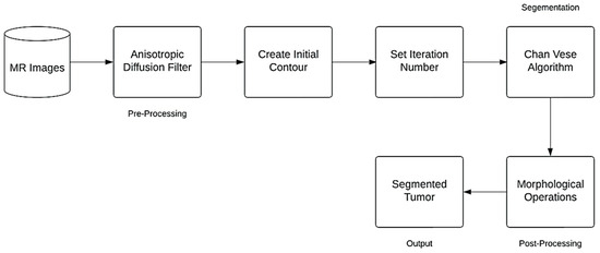
Figure 1.
Flowchart of the Proposed Method.
2.2.1. Anisotropic Diffusion Filter
In image processing and computer vision, anisotropic diffusion (see Figure 1), also called Perona-Malik diffusion, is a technique aimed at reducing image noise without removing significant parts of the image content—typically edges, lines, or other details that are important for the interpretation of the image [32,33].
Formally, let Ω ⊂ R2 denote a subset of the plane and ( , t): Ω → R be a family of gray scale images. ( ,0) is the input image. The anisotropic diffusion is defined as
where I is the intensity of the image and t is the time, Δ represents the Laplacian, ∇ represents the gradient, div (…) is the divergence operator. In vector calculus, divergence is a vector operator that operates on a vector field, producing a scalar field giving the quantity of the vector field’s source at each point, and c (x, y, t) is the diffusion coefficient
For t > 0 the output image is available as ( ,t) with the larger t producing blurrier images. Usually selected as a function of the picture gradient to retain edges in the image, (x, y, t) determines the rate of diffusion. In 1990 Pietro Perona and Jitendra Malik invented the concept of anisotropic diffusion and suggested two uses for the diffusion coefficient:
where K is a constant selected to improve the edge detection.
2.2.2. Contour Initialization
We used the “Radius Contraction and Expansion” technique to determine the initial shape of the active contour model. Contracting the radius generates a circular outline close to the region of interest, while expanding the radius facilitates contour movement and causes the radius to contract away from the area of interest [23].
2.2.3. Chan-Vese Algorithm
The Chan Vese algorithm is based on minimizing the energy function F (c1, c2, C) defined by Equation (3). The image xo comprises two areas with roughly constant levels for c1 and c2, c1 will denote the average pixels’ intensity inside C, and c2 will denote the average intensity outside C, where C denotes any variable curve [34]. Furthermore, assume a hypothetical expression in which the region represents the target object (i.e., the tumor) denoted as c1, with its boundary delineated by uo. The following equation formulates the Chan-Vese optimization method:
where , are fixed parameters (should be determined by the user). The relative balance between and determine which side, inside or outside has higher importance in minimizing the regional variance. As suggested by the paper, we choose the preferred settings as .
The first integral in Equation (3) range is inside C; the second integral in Equation (3) range is outside C. It should be noted that the term Length (C) could be re-written more generally as for p ≥ 1, but here we choose p = 1.
We are looking for c1, c2, and C that minimize the function F (c1, c2, C). For complete mathematical development refer to [34].
2.2.4. Post-Processing Method
The morphological operations on the binary image after the “Chan-Vese” method were used to help separate the tumor. We set the distance from the starting point of the structure element to the disk shape points in both cases to seven, and we set the distance for morphological expansion by dilation to eight. Additionally, we set the morphological erosion distance to seven, these values were chosen upon experimental testing. We use the disk form for morphological dilation and erosion because it performs better than other shapes like diamonds, squares, and lines.
2.3. Performance Evaluation Measures
The analysis of the experiment was performed according to the following performance parameters:
2.3.1. Accuracy
Accuracy measures the percentage of pixels in the brain tumor image that were correctly identified [35,36].
where TP is true positive, TN is true negative, FP is false positive, and FN is false negative. The same parameters are used in the equations below.
2.3.2. Precision
Precision accurately defines the purity of our positive detections of brain tumors in comparison to the ground truth image [7].
2.3.3. Sensitivity
Sensitivity, also called true positive rate, is the percentage of true positive values that are accurately detected [36,37].
2.3.4. Specificity
Compared to sensitivity, specificity or the true negative rate is a percentage of correctly detected negative values [36].
2.3.5. Jaccard Index
It is a measure of similarity between two sets of data that is simple to get interrupted [37].
2.3.6. Dice Index Coefficient
It is used to demonstrate the degree of similarity between the collected tumor and the manually segmented tumor area [37].
2.3.7. Hausdorff Distance
The segmentation method calculates the distance between the ground truth contour (A) and the segmented contour (B). The segmentation method produces the best results when the Hausdorff distance is near zero [37].
HD (A, B) = max (min||A-B||)
The generalized Hausdorff measure provides the most effective techniques for comparing specific areas of one image with another. Often, the matching process involves subjecting the two images to some form of geometric transformation. In this metric, the percentage of points in one set that are close to points in the other measures how similar two point sets are. Consequently, two factors determine the similarity of two point sets: the minimum distance required for points to be considered close together, and the percentage of points that are (at most) this close distance apart from points in the other set. The absence of point pairing in the two sets under comparison distinguishes this distance measure from correspondence-based methods such as binary correlation and point matching techniques.
3. Results
This section presents the results in Figure 2 for single image, we comparing the effect of the filter of the proposed method as shown in Table 1, while the performance measures presented in Table 2 and Figure 3, Figure 4 and Figure 5 are the average of performance measures obtained from all 50 cases.
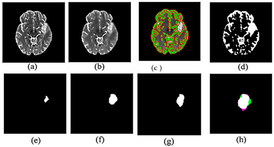
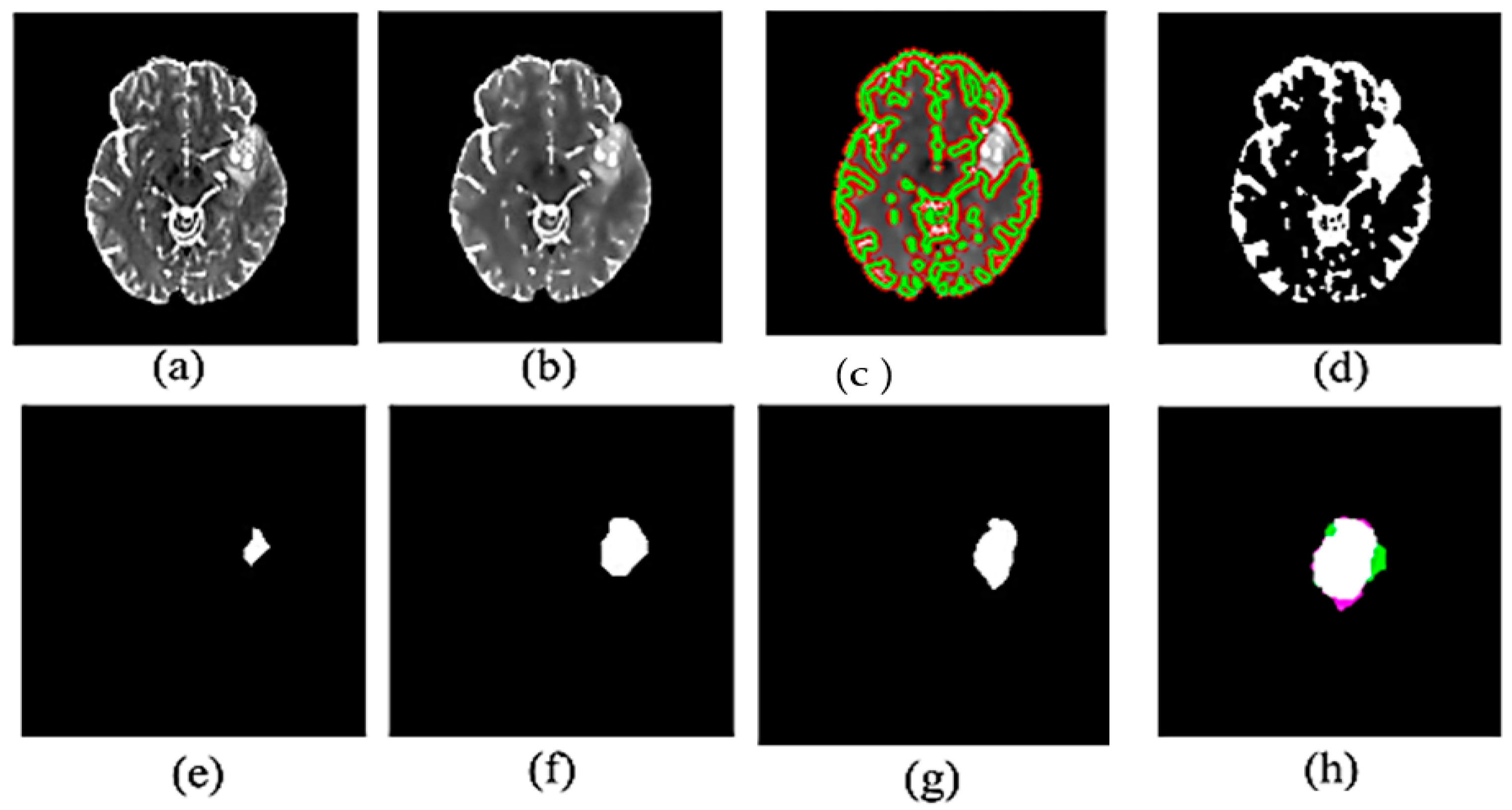
Figure 2.
Experimental results for proposed method: (a) Input MR image (b) Filtered image (c) Brain image after contour detection (d) Segmented binary image (e) eroded MR image in (d,f) dilated MR image of (e,g) Ground truth of tumor (h) Combine the ground truth and the segmented tumor.

Table 1.
Comparing the effect of the filter in the proposed method (“Chan-Vese”).
Table 2.
Performance evaluation measure of two methods vs. proposed method.

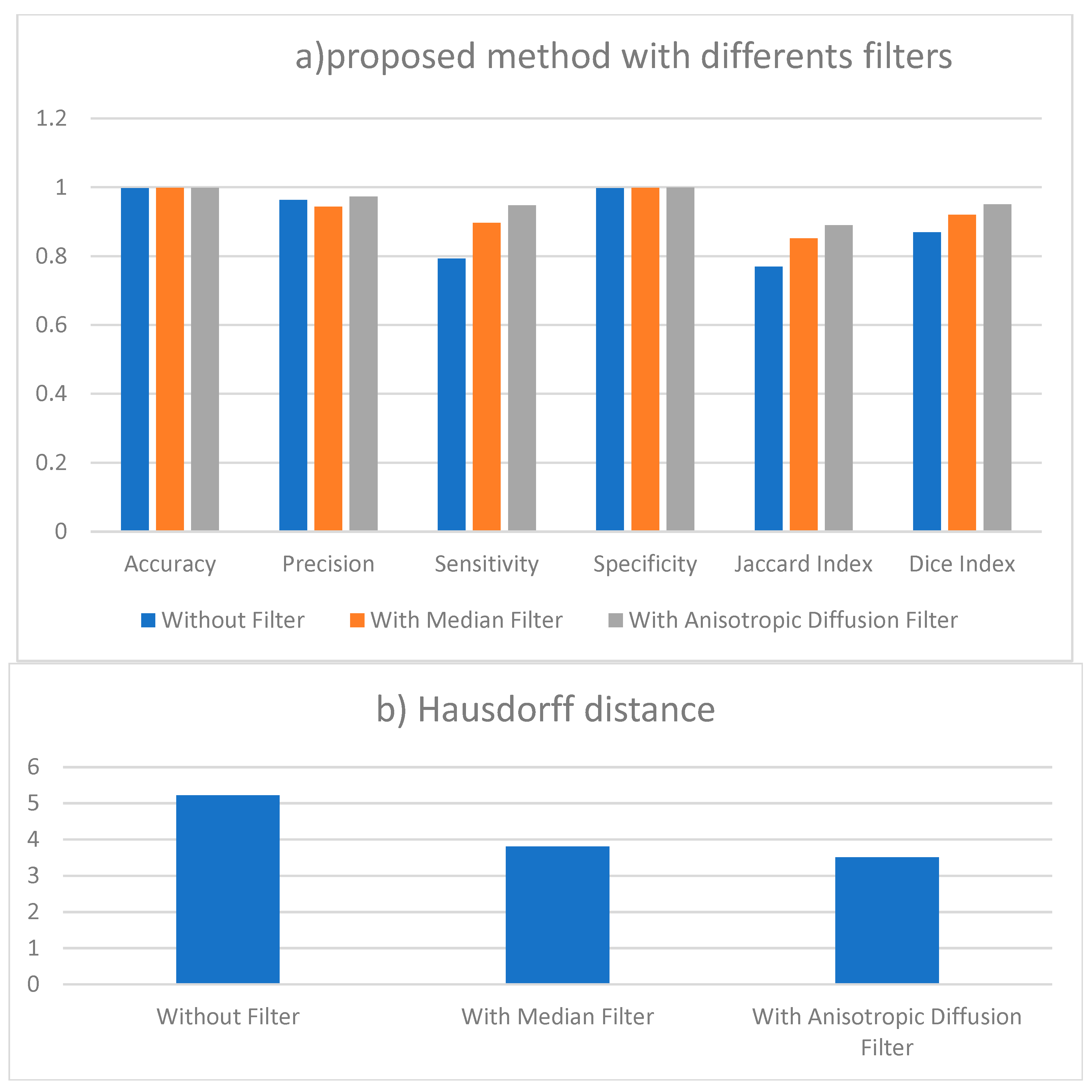
Figure 3.
(a) Performance measures of proposed method results without filter and with two different filtering. (b) Results of Hausdorff distance for segmentation with different filters.

Figure 4.
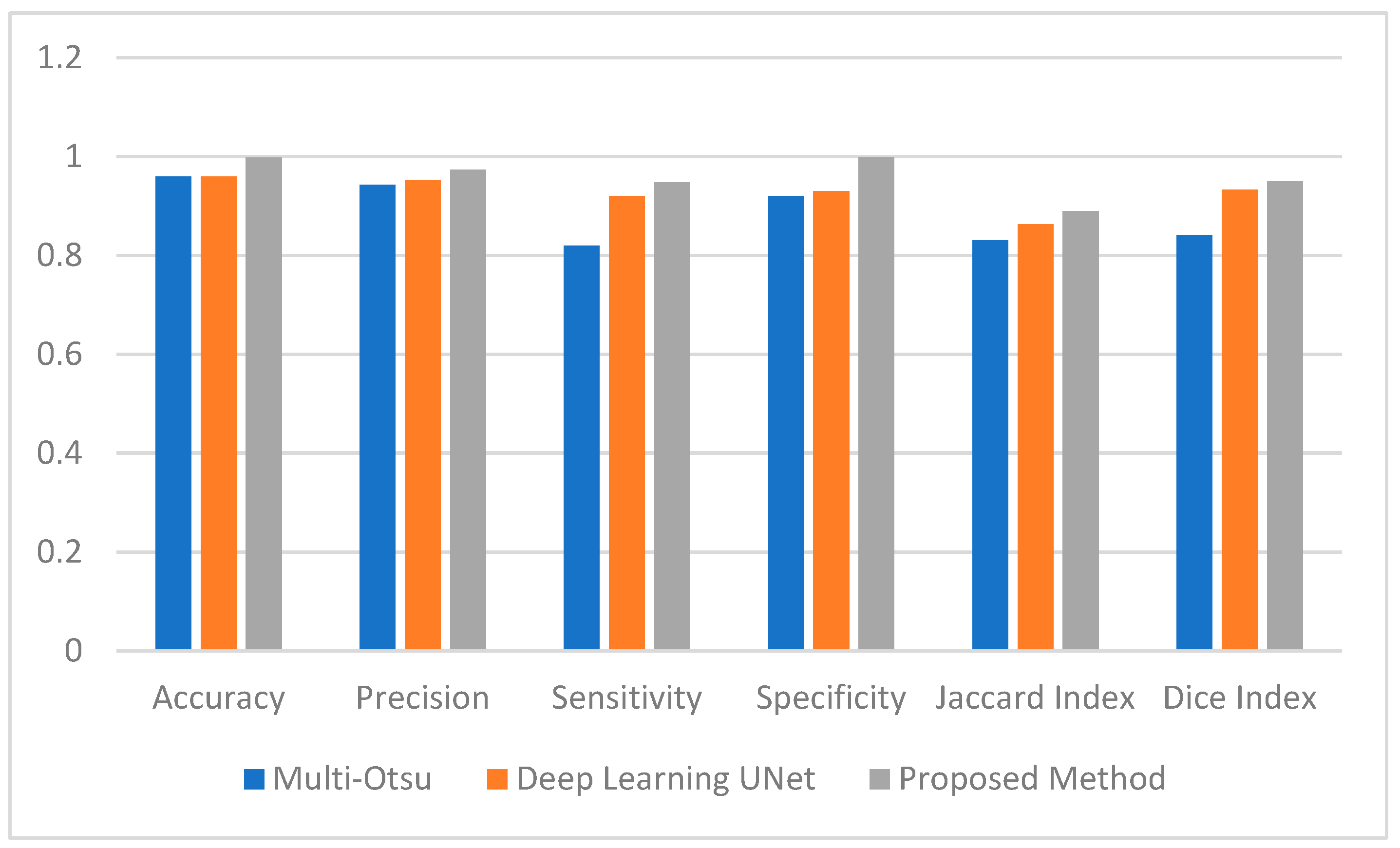
Average Performance Measure comparison between the Muli-Otsu, UNet and proposed method.

Figure 5.
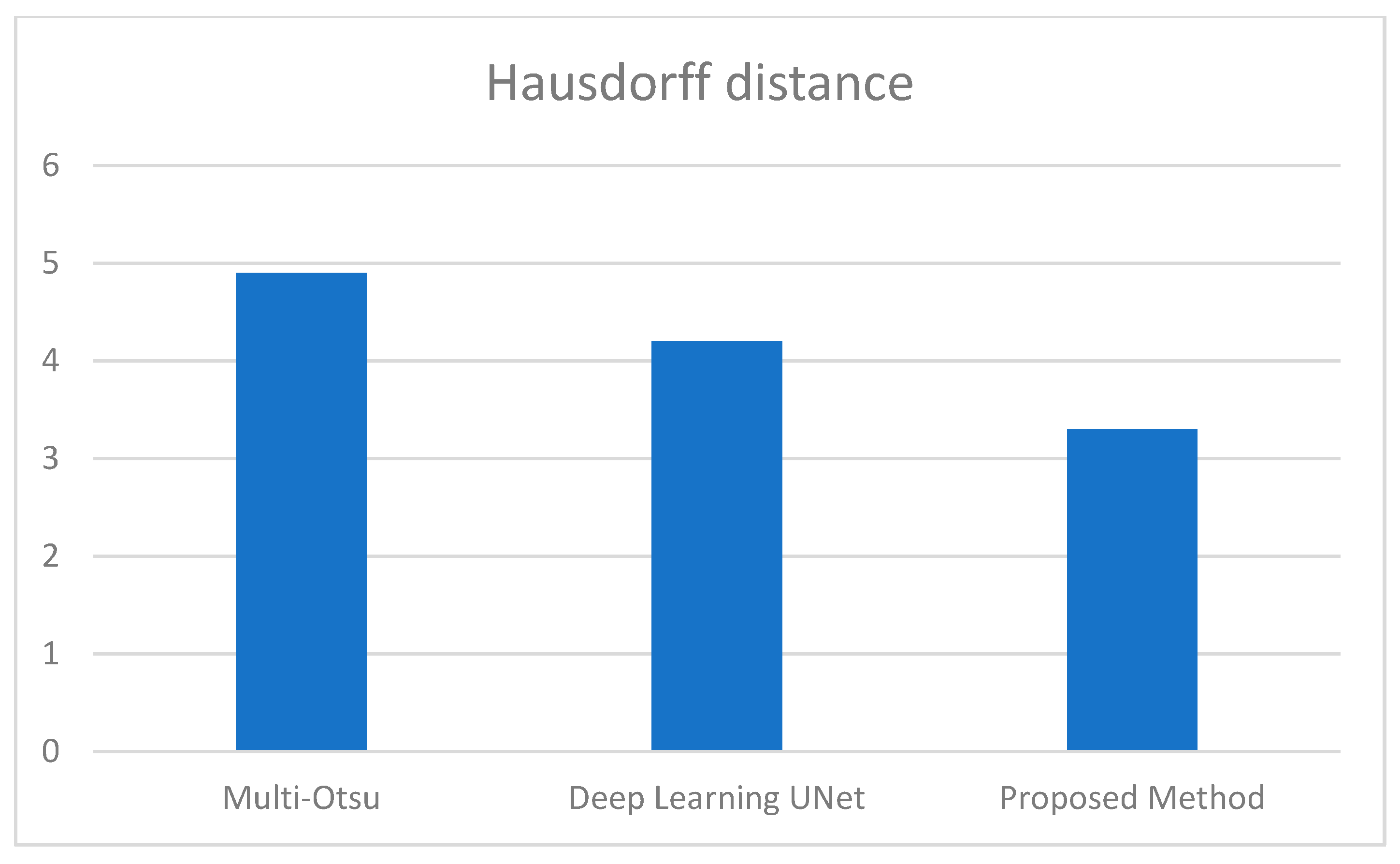
Average Hausdorff distance comparison between the 3 methods.
3.1. Proposed Method Results
Figure 2 illustrates the visual results of the proposed method. Figure 2a,b show the original image from the dataset and the resultant image after applying anisotropic diffusion, respectively. After applying the initial contour, Figure 2c displays the segmented image with a green color contour surrounding the suggested tumor, while Figure 2d displays the binary image derived from Figure 2c. We then performed morphological procedures using an 8-radius disc shape for erosion, as shown in Figure 2e, and a 7-radius disc shape for dilation, as illustrated in Figure 2f. Incorporating these morphological processes is a crucial element in the post-processing stage of the segmentation. Figure 2g and Figure 2h, respectively, illustrate the ground truth tumor and the combination of the segmented tumor and ground truth.
Furthermore, the green area in Figure 2h shows false positive pixels—areas found in the segmented image but not in the ground truth that show malignancies. False negative pixels in the purple area indicate areas of ground truth where tumors are present but not found in the segmented image.
The results presented in Table 1 are the average obtained from the 50 individual images.
3.2. Performance Evaluation Measures Results
The Deep Learning UNet and the Multi-Otsu algorithms where implemented using the same dataset as the proposed method for the purpose of comparison [25].
This section employs numerical data to clarify the testing results of the utilized methodologies. Figure 4 provides a visual representation of the effectiveness of the segmentation strategies as evaluated by a range of performance criteria. According to the data presented in Figure 4, the multi-Otsu segmentation method achieves an accuracy rate of 96%. However, the proposed method demonstrates a higher accuracy rate of 99%. Moreover, the mean sensitivity and specificity values for multi-Otsu segmentation are 82% and 92%, respectively. In contrast, these values are 95% and 99% for the proposed method, and 92% and 93% for the deep learning UNet method.
We additionally examined the Jaccard index and dice score to enable an in-depth analysis of the proposed approaches. Consequently, the average Jaccard index and dice score obtained by the proposed method are 89% and 95%, respectively. Similarly, multi-Otsu segmentation measured the same metrics at 83% and 84%, respectively. The results of the deep learning method UNet are 86% and 87%, respectively. Furthermore, Figure 5 presents the mean Hausdorff distance for the multi-level Otsu, UNet, and proposed method. The three methods demonstrate an average Hausdorff distance of 4.9, 4.2, and 3.3, respectively. Specifically, we consider the segmentation method optimal when the Huasdorff distance approaches zero.
4. Discussion
Table 1 lists the statistical measures of sensitivity, accuracy, and precision applied in evaluation of the classifier’s performance. Moreover, better performance is shown by higher sensitivity and accuracy ratings. Fifty photos have been divided. With a standard deviation of 0.07 percent, the average accuracy of the whole photographic collection is 99.5 percent. This shows the great accuracy of the segmentation. With a standard variation of about 3.5 per-cent, the average precision is about 97.5 percent. With a standard deviation range of around 3.4 percent, the average Dice result is almost 87 percent. With a standard deviation of about 5 percent, the average sensitivity is about 93 percent. Including all four performance evaluation criteria, the average estimate of tumor detection comes out to be about 94.5 percent. These findings show that our segmentation technique performs rather well. Even a modest enhancement in the sensitivity parameter for surgical planning is much needed by radiologists or clinical doctors.
We evaluated our results against several new and time-consuming techniques including neural network and deep learning methods (Single Path MLDeepMedic, U-Net, Rescue Net, and Cascaded Anistropic CNN), as well as some classical segmentation methods. Our results matched generally used methods implemented in recent years. Table 3 provides a comparison of various approaches on the same dataset (BTS 2017–2021) together with the dice index performance. We chose the dice index since it is widely used in the literature and since results for all compared approaches are easily available. Although all the evaluated techniques employ the same database dataset, the quantity of photos in our experimental data differs from the others.
Table 3.
Summary of some brain segmentation methods and their validation metrics.
We compare the average dice index of 50 photographs to others. The techniques such as Otsu’s thresholding, k-means clustering, and fuzzy K-means have demonstrated commendable performance, with an accuracy rate that ranges from 84.72% to almost 89% of the higher dice coefficient. This indicates a strong correlation with accurate manual segmentation of tumor regions. A hybrid approach to managing variability in MRI data was demonstrated using an Otsu combined for FCM that has obtained an accuracy of 90.57%.
On average, the computational time of the proposed method took approximately 4 min to complete the entire pipeline when running on a desktop, CPU i7 and 8 GiB of Memory RAM). In contrast, the deep learnings software, using google Colabt service, it took a time for one epoch between 30 s to 50 s, the total time for 50 Epochs it took between 30 to 42 min as shown in the table above.
Table 3 shows that our suggested method works better than unsupervised techniques like K-means and FCM, as well as traditional segmentation methods like Otsu’s thresholding, Chan-Vese, and multilevel HSO [25]. It produces better results than some deep learning techniques, such UNet, cascaded anisotropic CNN. For unsupervised segmentation, the suggested system produces results fast, outperforming fuzzy clustering and matching performance to current neural network methods such U-Net and cascaded anisotropic CNN and single-path ML deepMeic. It performs somewhat less than the supervised deep learning method known as the Rescue Net approach, which calls for a large dataset for learning and a lot of processing time. It also consumes a lot of CPU capability and memory.
Figure 2 presents the qualitative segmentation results for the BraTS 2021 dataset. Our method effectively segments complete tumor regions, as demonstrated in the images. The study indicated that certain artifacts in abnormal brain tumor images remained despite the application of pre-processing and segmentation techniques. We employed post-processing techniques like morphological dilation and erosion to identify brain tumors of suitable size and eliminate artifacts. The suggested method works better than traditional segmentation methods because it combines anisotropic diffusion filtering, Chan-Vese segmentation, and post-processing. It also surpasses certain deep learning approaches, as shown in Table 2, when evaluated using Jaccard and Dice indices and Hausdorff distance.
However, the shortcomings of the proposed method arise in various scenarios, such as large tumors, where the 2D images may not accurately depict the tumor’s central slice, necessitating further tracing of the central section. Generally, a 2D picture does not capture the 3D dimension of a tumor, so we should extend the method to 3D MRI data for more accurate segmentation. Some deep learning methods like “U-Net++DSM” method [38,39], which utilizes the U-Net architecture. This reference reports impressive performance metrics for brain tumor segmentation. • Sensitivity: 98.59% • Specificity: 98.64% • Accuracy: 98.64% • Dice Score: 98.02% which have the potential to outperform the proposed approach by up to 2.4%. However, these methods come with significantly higher costs for training and evaluation, including computational time, computer system hardware and software, memory, graphic cards, and CPU. An average desktop may take several hours for training and validation (15 hrs) of run time; the deep learning algorithm usually runs on Google Colab.5. to speed up the process.
5. Conclusions
The preliminary findings of our technique show great potential in aiding physicians in real-time estimation of the precise location and dimensions of MRI brain tumors. Moreover, it is quasi-automatic and does not need training. The only fixed parameter is the prescribed number of levels for the segmentation. Comparing the results with other recently published approaches in the literature shows that the proposed method is highly promising as an artificial intelligence application for brain tumor identification. Future research must assess the effectiveness of these segmentation methods across various brain tumor types and enhance computational efficiency to incorporate the technology into clinical processes.
Author Contributions
Conceptualization, A.S.S.; methodology, A.S.S. and M.A.; software, F.A.A. and G.F.A.; writing—original draft preparation, F.A.A., G.F.A. and A.S.S.; writing—review and editing, M.A., Z.A. and O.A.; visualization, F.A.A. and G.F.A.; supervision, A.S.S.; project administration, M.A.; funding acquisition, M.A., Z.A. and O.A. All authors have read and agreed to the published version of the manuscript.
Funding
This research was funded by the College of Applied Medical Sciences Research Centre and the Deanship of Scientific Research at King Saud University.
Data Availability Statement
Available upon request from the corresponding author.
Acknowledgments
The authors extend their appreciation to the College of Applied Medical Sciences Research Centre and the Deanship of Scientific Research at King Saud University for its funding for this research.
Conflicts of Interest
The authors declare no conflicts of interest.
References
- Saini, A.; Kumar, M.; Bhatt, S.; Saini, V.; Malik, A. Cancer causes and treatments. Int. J. Pharm. Sci. Res. 2020, 11, 3121–3134. [Google Scholar]
- Shah, V.; Kochar, P. Brain cancer: Implication to disease, therapeutic strategies and tumour targeted drug delivery approaches. Recent Pat. Anti-Cancer Drug Discov. 2018, 13, 70–85. [Google Scholar] [CrossRef] [PubMed]
- Patel, A. Benign vs malignant tumours. JAMA Oncol. 2020, 6, 1488. [Google Scholar] [CrossRef] [PubMed]
- Amin, J.; Sharif, M.; Yasmin, M.; Fernandes, S.L. A distinctive approach in brain tumour detection and classification using MRI. Pattern Recognit. Lett. 2020, 139, 118–127. [Google Scholar] [CrossRef]
- Moser, E.; Stadlbauer, A.; Windischberger, C.; Quick, H.H.; Ladd, M.E. Magnetic resonance imaging methodology. Eur. J. Nucl. Med. Mol. Imaging 2009, 36, 30–41. [Google Scholar] [CrossRef]
- Manikandan, R.; Monolisa, G.; Saranya, K. A cluster based segmentation of magnetic resonance images for brain tumour detection. Middle-East J. Sci. Res. 2013, 14, 669–672. [Google Scholar]
- Lerch, J.P.; van der Kouwe, A.J.W.; Raznahan, A.; Paus, T.; Johansen-Berg, H.; Miller, K.L.; Smith, S.M.; Fischl, B.; Sotiropoulos, S.N. Studying neuroanatomy using MRI. Nat. Neurosci. 2017, 20, 314–326. [Google Scholar] [CrossRef]
- Bejer-Oleńska, E.; Wojtkiewicz, J. Utilization of MRI technique in the patient population admitted between 2011 and 2015 to the University Clinical Hospital in Olsztyn. Pol. Ann. Med. 2017, 24, 199–204. [Google Scholar] [CrossRef]
- Vasung, L.; Turk, E.A.; Ferradal, S.L.; Sutin, J.; Stout, J.N.; Ahtam, B.; Lin, P.-Y.; Grant, P.E. Exploring early human brain development with structural and physiological neuroimaging. Neuroimage 2018, 187, 226–254. [Google Scholar] [CrossRef]
- Yousaf, T.; Dervenoulas, G.; Politis, M. Advances in MRI methodology. Int. Rev. Neurobiol. 2018, 141, 31–76. [Google Scholar]
- Jalab, H.A.; Hasan, A.M. Magnetic resonance imaging segmentation techniques of brain tumours: A review. Arch. Neurosci. 2019, 6, e84920. [Google Scholar] [CrossRef]
- Harouni, M.; Karimi, M.; Rafieipour, S. Precise segmentation techniques in various medical images. In Artificial Intelligence and Internet of Things; CRC Press: Boca Raton, FL, USA, 2021; pp. 117–166. [Google Scholar]
- Havaei, M.; Davy, A.; Warde-Farley, D.; Biard, A.; Courville, A.; Bengio, Y.; Pal, C.; Jodoin, P.-M.; Larochelle, H. Brain tumour segmentation with deep neural networks. Med. Image Anal. 2017, 35, 18–31. [Google Scholar] [CrossRef] [PubMed]
- Işın, A.; Direkoğlu, C.; Şah, M. Review of MRI-based brain tumour image segmentation using deep learning methods. Procedia Comput. Sci. 2016, 102, 317–324. [Google Scholar] [CrossRef]
- Rafi, A.; Khan, Z.; Aslam, F.; Jawed, S.; Shafique, A.; Ali, H. A review: Recent automatic algorithms for the segmentation of brain tumour MRI. In AI and IoT for Sustainable Development in Emerging Countries: Challenges and Opportunities; Springer: Berlin/Heidelberg, Germany, 2022; pp. 505–522. [Google Scholar]
- Ranjbarzadeh, R.; Caputo, A.; Tirkolaee, E.B.; Ghoushchi, S.J.; Bendechache, M. Brain tumour segmentation of MRI images: A comprehensive review on the application of artificial intelligence tools. Comput. Biol. Med. 2023, 152, 106405. [Google Scholar] [CrossRef]
- Wadhwa, A.; Bhardwaj, A.; Verma, V.S. A review on brain tumour segmentation of MRI images. Magn. Reson. Imaging 2019, 61, 247–259. [Google Scholar] [CrossRef]
- Kaur, A. An automatic brain tumour extraction system using different segmentation methods. In Proceedings of the 2016 Second International Conference on Computational Intelligence & Communication Technology (CICT), Ghaziabad, India, 12–13 February 2016; pp. 187–191. [Google Scholar]
- Otsu, N. A threshold selection method from gray-level histograms. IEEE Trans. Syst. Man Cybern. 1979, 9, 62–66. [Google Scholar] [CrossRef]
- Rao, C.S.; Karunakara, K. A comprehensive review on brain tumour segmentation and classification of MRI images. Multimed. Tools Appl. 2021, 80, 17611–17643. [Google Scholar] [CrossRef]
- Tripathi, P.; Singh, V.K.; Trivedi, M.C. Brain tumour segmentation in magnetic resonance imaging using OKM approach. Mater. Today Proc. 2021, 37, 1334–1340. [Google Scholar] [CrossRef]
- Babu, K.; Indira, N.; Prasad, K.V.; Shameem, S. An effective brain tumour detection from t1w MR images using active contour segmentation techniques. J. Phys. Conf. Ser. 2021, 1804, 012174. [Google Scholar] [CrossRef]
- Sheela, C.J.J.; Suganthi, G. Brain tumour segmentation with radius contraction and expansion based initial contour detection for active contour model. Multimed. Tools Appl. 2020, 79, 23793–23819. [Google Scholar] [CrossRef]
- Sheela, C.J.J.; Suganthi, G. Automatic brain tumour segmentation from MRI using greedy snake model and fuzzy C-means optimization. J. King Saud Univ. Comput. Inf. Sci. 2022, 34, 557–566. [Google Scholar] [CrossRef]
- Aleid, A.; Alhussaini, K.; Alanazi, R.; Altwaimi, M.; Altwijri, O.; Saad, A.S. Artificial Intelligence Approach for Early Detection of Brain Tumors Using MRI Images. Appl. Sci. 2023, 13, 3808. [Google Scholar] [CrossRef]
- Iqbal, S.; Qureshi, A.N.; Li, J.; Mahmood, T. On the analyses of medical images using traditional machine learning techniques and convolutional neural networks. Arch. Comput. Methods Eng. 2023, 30, 3173–3233. [Google Scholar] [CrossRef]
- Tandel, G.S.; Biswas, M.; Kakde, O.G.; Tiwari, A.; Suri, H.S.; Turk, M.; Laird, J.R.; Asare, C.K.; Ankrah, A.A.; Khanna, N.N.; et al. A review on a deep learning perspective in brain cancer classification. Cancers 2019, 11, 111. [Google Scholar] [CrossRef] [PubMed]
- Aamir, M.; Namoun, A.; Munir, S.; Aljohani, N.; Alanazi, M.H.; Alsahafi, Y.; Alotibi, F. Brain Tumor Detection and Classification Using an Optimized Convolutional Neural Network. Diagnostics 2024, 14, 1714. [Google Scholar] [CrossRef] [PubMed]
- Menze, B.H.; Jakab, A.; Bauer, S.; Kalpathy-Cramer, J.; Farahani, K.; Kirby, J.; Burren, Y.; Porz, N.; Slotboom, J.; Wiest, R.; et al. The multimodal brain tumour image segmentation benchmark (BRATS). IEEE Trans. Med. Imaging 2014, 34, 1993–2024. [Google Scholar] [CrossRef]
- Bakas, S.; Akbari, H.; Sotiras, A.; Bilello, M.; Rozycki, M.; Kirby, J.S.; Freymann, J.B.; Farahani, K.; Davatzikos, C. Advancing the cancer genome atlas glioma MRI collections with expert segmentation labels and radiomic features. Sci. Data 2017, 4, 1–13. [Google Scholar] [CrossRef]
- Bakas, S.; Akbari, H.; Sotiras, A.; Bilello, M.; Rozycki, M.; Kirby, J.S.; Freymann, J.B.; Farahani, K.; Davatzikos, C. Segmentation labels and radiomic features for the pre-operative scans of the TCGA-LGG collection. Cancer Imaging Arch. 2017. [Google Scholar] [CrossRef]
- Perona, P.; Malik, J. Scale-space and edge detection using anisotropic diffusion. In Proceedings of the IEEE Computer Society Workshop on Computer Vision, Miami Beach, FL, USA, 30 November–2 December 1987; pp. 16–22. [Google Scholar]
- Perona, P.; Malik, J. Scale-space and edge detection using anisotropic diffusion (PDF). IEEE Trans. Pattern Anal. Mach. Intell. 1990, 12, 629–639. [Google Scholar] [CrossRef]
- Chan, T.F.; Vese, L.A. Active contours without edges. IEEE Trans. Image Process. 2001, 10, 266–277. [Google Scholar] [CrossRef]
- Towards Data Science. How to Evaluate Image Segmentation Models. Medium. Towards Data Science. 2020. Available online: https://towardsdatascience.com/how-accurate-is-image-segmentation-dd448f896388 (accessed on 20 January 2022).
- Fernandes, S.L.; Tanik, U.J.; Rajinikanth, V.; Karthik, K.A. A reliable framework for accurate brain image examination and treatment planning based on early diagnosis support for clinicians. Neural Comput. Appl. 2020, 32, 15897–15908. [Google Scholar] [CrossRef]
- Sheela, C.J.J.; Suganthi, G. Accurate MRI brain tumour segmentation based on rotating triangular section with fuzzy C-means optimization. Sādhanā 2021, 46, 226. [Google Scholar] [CrossRef]
- Wisaeng, K. U-Net++DSM: Improved U-Net++ for brain tumor segmentation with deep supervision mechanism. IEEE Access 2023, 11, 132268–132285. [Google Scholar] [CrossRef]
- Umarani, C.M.; Gollagi, S.G.; Allagi, S.; Sambrekar, K.; Ankali, S.B. Advancements in deep learning techniques for brain tumor segmentation: A survey. Inform. Med. Unlocked 2024, 50, 101576. [Google Scholar] [CrossRef]

Disclaimer/Publisher’s Note: The statements, opinions and data contained in all publications are solely those of the individual author(s) and contributor(s) and not of MDPI and/or the editor(s). MDPI and/or the editor(s) disclaim responsibility for any injury to people or property resulting from any ideas, methods, instructions or products referred to in the content. |
© 2025 by the authors. Licensee MDPI, Basel, Switzerland. This article is an open access article distributed under the terms and conditions of the Creative Commons Attribution (CC BY) license (https://creativecommons.org/licenses/by/4.0/).