Abstract
The conventional diagnostic techniques for ethylene cracker furnace tube coking rely on manual expertise, offline analysis and on-site inspection. However, these methods have inherent limitations, including prolonged inspection times, low accuracy and poor real-time performance. This makes it challenging to meet the requirements of chemical production. The necessity for high efficiency, high reliability and high safety, coupled with the inherent complexity of the production process, results in data that is characterized by multimodal, nonlinear, non-Gaussian and strong noise. This renders the traditional data processing and analysis methods ineffective. In order to address these issues, this paper puts forth a novel soft measurement approach, namely the ‘Mixed Student’s t-distribution regression soft measurement model based on Variational Inference (VI) and Markov Chain Monte Carlo (MCMC)’. The initial variational distribution is selected during the initialization step of VI. Subsequently, VI is employed to iteratively refine the distribution in order to more closely approximate the true posterior distribution. Subsequently, the outcomes of VI are employed to initiate the MCMC, which facilitates the placement of the iterative starting point of the MCMC in a region that more closely approximates the true posterior distribution. This approach allows the convergence process of MCMC to be accelerated, thereby enabling a more rapid approach to the true posterior distribution. The model integrates the efficiency of VI with the accuracy of the MCMC, thereby enhancing the precision of the posterior distribution approximation while preserving computational efficiency. The experimental results demonstrate that the model exhibits enhanced accuracy and robustness in the diagnosis of ethylene cracker tube coking compared to the conventional Partial Least Squares Regression (PLSR), Gaussian Process Regression (GPR), Gaussian Mixture Regression (GMR), Bayesian Student’s T-Distribution Mixture Regression (STMR) and Semi-supervised Bayesian T-Distribution Mixture Regression (SsSMM). This method provides a scientific basis for optimizing and maintaining the ethylene cracker, enhancing its production efficiency and reliability, and effectively addressing the multimodal, non-Gaussian distribution and uncertainty of the coking data of the ethylene cracker furnace tube.
1. Introduction
The significance of ethylene in the petrochemical industry is increasing in tandem with the ongoing advancement of society and the economy [1,2,3]. In the context of industrial production, ethylene is derived from naphtha and other raw materials under conditions of anaerobic or low oxygen content. This is achieved through the process of cracking, whereby carbon–carbon and carbon–hydrogen bonds are broken at elevated temperatures. In order to enhance the safety and efficacy of ethylene cracker production, it is imperative to implement a comprehensive monitoring system for the ethylene production process. However, the elevated temperature, pressure, flammability and explosivity inherent to the production of ethylene columns render direct measurement of certain operational parameters, such as furnace temperature, challenging. With the development of artificial intelligence technology, people have started to try to model the ethylene cracker modeling and they are trying to monitor it through artificial intelligence (AI) methods. By simulating the coking process, establishing a detailed mechanism model and exploring the optimal control strategy as well as the simulation and automatic control technology of the coke clearing process, these results demonstrate the progress made in improving the operating efficiency of cracker furnaces, prolonging the service life of furnace tubes and achieving an accurate diagnosis, and at the same time point out the directions that still need further research and improvement in practical applications [4,5,6]. Therefore, it is imperative that fast, accurate and stable ethylene cracking stovepipe models are developed in order to advance production intelligence [7]. Nevertheless, the high-temperature cracking catalytic generation process of ethylene is inherently complex, rendering it more challenging to develop a comprehensive model of the ethylene cracking process.
The challenge and uniqueness of directly measuring the pertinent variables may impact the precision of sample matching. Soft measurement technology enables the real-time monitoring of crucial process parameters without the necessity for costly sensors or intricate measurement apparatus, thereby enhancing the accuracy and efficiency of data processing. This technology is extensively utilized in the chemical industry and other domains [8,9,10]. The estimation of the dominant variable through the use of auxiliary variables is a common practice in soft measurement techniques. However, when the auxiliary variables are multidimensional and exhibit inconsistent effects, the resulting prediction error is likely to be amplified [11,12,13]. In general, soft measurement methods are classified into two main categories: mechanistic model-based and data-driven [14]. In the case of the ethylene cracker, the mechanistic modeling approach is, by its very nature, strongly interpretative and complex. Furthermore, it requires precise parameters that are difficult to measure and model [15,16]. In contrast, data-driven approaches employ historical data and machine learning algorithms that are not contingent on a priori knowledge and are therefore well-suited to the analysis of complex and uncertain systems [17,18]. Consequently, mechanistic model are typically well-suited for elucidating the fundamental mechanisms, whereas data-driven methodologies are more appropriate for addressing the intricacies and uncertainties inherent to the system [19]. However, the data obtained from the ethylene cracker production process are characterized by multimodality, nonlinearity, non-Gaussianity and strong noise [20], which necessitates the utilization of advanced methods and techniques to facilitate its analysis. A comparison of the mechanistic and data-driven models is shown in Table 1.

Table 1.
Comparison of mechanistic and data-driven models.
In the field of statistical modeling and machine learning, the mixed Student’s t-distribution regression models have been the subject of considerable interest due to their resilience to outliers and their capacity to accommodate multimodal data effectively. The model is capable of capturing both heteroskedasticity and the heavy-tailed nature of the data. Therefore, it is also widely used in a number of fields, including finance, bioinformatics and signal processing.
The prevalence of outliers in industrial data renders traditional analyses based on Gaussian distribution vulnerable to interference. In contrast, the Student’s t-distribution, due to its thicker tails and lower sensitivity to outliers, is better suited to handle this type of data, thus improving the robustness and accuracy of the analysis [21]. Nevertheless, the estimation of its parameters necessitates the performance of intricate integration operations, rendering the application of traditional maximum likelihood estimation a challenging undertaking. To overcome this challenge, researchers have proposed a variety of Bayesian inference methods, among which VI and MCMC are two mainstream solutions. While VI and MCMC each possess distinctive advantages in addressing complex models, they also exhibit inherent limitations. As a Bayesian approximation method, VI is efficient but contingent upon the precision of the variational distribution, potentially inadequate for accurately approximating the posterior distribution. Conversely, MCMC, while theoretically capable of accurately recovering the posterior probabilities, is computationally inefficient, may require an extended convergence period, and is costly to process large data sets [22,23]. In light of the aforementioned considerations, this paper puts forth a novel approach that integrates VI and MCMC. This integration aims to enhance the efficacy and precision of parameter estimation in mixed Student’s t-distribution regression models [24].
This paper presents an overview of the Student’s T-Distribution Mixture Regression model and its associated parameter estimation challenges. It also outlines a proposed alternating iteration method and provides experimental verification of its advantages in terms of parameter estimation, prediction accuracy, and computational efficiency.
In summary, the main contributions of this paper are as follows:
- We developed an algorithm called variational Bayesian MCMC (VM), which consists of VI and MCMC;
- Our VM introduces the Student’s t-distribution, which provided robust classification results;
- In order to determine whether the proposed method is effective, it is necessary to use two sets of data that contain different categories as a basis for the experiment.
2. Related Works
In recent years, soft measurement techniques have assumed an increasingly pivotal role in industrial process control, particularly in the estimation of critical quality parameters that are challenging to measure directly. Conventional soft measurement techniques, such as those based on inference and control through mechanistic modeling, can satisfy the aforementioned demand to a certain extent. However, their efficacy is frequently constrained by the precision and practicality of the model employed. For example, Hongye Jiang et al. (2023) [25] proposed a new corrosion prediction mechanism model for predicting the corrosion rate of a gathering pipeline in a carbon dioxide environment. This model was validated by comparing it with experimental data, and it demonstrated good prediction accuracy. However, the accuracy of this model depends on the availability of high-quality experimental data. Conversely, Shaochen Wang et al. (2023) [26] integrated deep learning methodologies with a model based on the distillation process mechanism. This approach has the potential to markedly enhance the safety, stability, and reliability of the production system. However, it necessitates substantial computational resources, which may present a challenge in practical applications. The advancement of artificial intelligence has led to a growing interest in data-driven soft measurement methods based on data. To illustrate, the soft sensor framework proposed by Runyuan Guo et al. (2021) [27] employs a generative adversarial network (GAN) and gated recurrent unit (GRU) to enhance the precision and resilience of prediction. However, the intricacy of the model may compromise the dependability of its prediction outcomes. Similarly, the Long Short-Term Memory–Deep Factorization Machine (LSTM-DeepFM) model, a data-driven self-supervised approach proposed by Ren L et al. (2022) [19], combines the advantages of LSTM and DeepFM to capture data features with greater accuracy, thereby enhancing prediction and monitoring precision. However, the model structure is more complex and necessitates a substantial amount of data for effective training. The data-driven soft sensor approach proposed by He Z et al. (2022) [28] combines multiple machine learning algorithms, which enhances the efficiency and quality control of the papermaking process by monitoring key quality parameters in real time. However, the integration of multiple machine learning algorithms also elevates the complexity of the model and the challenge of maintenance. Notwithstanding the efficacy of these methodologies in addressing intricate data characteristics, such as nonlinearity, non-Gaussianity, and uncertainty, there remain a few challenges and constraints.
In the field of parameter estimation for mixed Student’s t-distribution regression model, researchers have primarily concentrated on the utilization of these methods to enhance model robustness and inference efficiency. For example, the Bayesian mixed model based on Student’s t-distribution proposed by Markus Svense’n et al. (2005) [29] displays good robustness in addressing outliers and is able to automatically determine the number of components in the mixed model. The mixed regression model (SMR) based on a Student’s t-distribution, as proposed by Jingbo Wang et al. (2018) [30], serves to enhance the robustness of the model to outliers; however, the computational complexity is considerable. The matching method based on a Bayesian mixed Student’s t-distribution model, as proposed by Lijuan Yang et al. (2018) [31], further improves the robustness to outliers through the optimization of the variational Bayesian framework. The semi-supervised robust modeling method (SsSMM), which is based on Student’s t-distribution mixture model and was proposed by Weiming Shao et al. (2019) [32], employs unlabeled data to address the issue of multimodal industrial processes. However, it should be noted that the method is more susceptible to parameter selection.
In recent years, there have been notable advancements in the field of Bayesian inference, particularly in the utilization of VI and MCMC, in addressing intricate statistical models. While VI and MCMC are commonly employed for parameter estimation in mixed Student’s t-distribution regression models, they each have their limitations.
The approximation accuracy of VI may be affected when dealing with a highly complex model. To illustrate, the variational Bayesian Gaussian Mixture Regression (VBGMR) method proposed by Jinlin Zhu et al. (2016) [17] is more efficient in model selection. However, the choice of prior distribution and model parameters significantly affects the results. The variational Bayesian Monte Carlo (VBMC) method proposed by Luigi Acerbi et al. (2018) [33] combines the VI advantages and reduces the number of required samples. Nevertheless, it may require fine parameter tuning and optimization. In a further development of the variational Bayesian approach, Jingbo Wang et al. (2019) [34] proposed a robust inference sensor development method based on variational Bayesian mixed Student’s t-distribution regression (VBSMR). This method is effective in identifying and reducing the impact of outliers on the prediction performance, but also requires consideration of its computational complexity and parameter selection challenges.
In contrast, while MCMC can provide accurate posterior estimates, the speed of convergence and the computational cost are often limiting factors. For example, Leandro Passos de Figueiredo et al. (2019) [35] proposed a method based on Gaussian mixture modeling and Markov Chain Monte Carlo to solve the linear ground seismic inversion problem. The method can effectively deal with non-Gaussian noise and complex data distributions through the Gaussian mixture model, which improves the accuracy of the inversion results. However, due to the need for a large number of samples, the computational cost of the method is high and the convergence speed is slow, which limits its efficiency in practical applications to some extent. Jonas Gregor Wiese et al. (2023) [36] proposed a new method for efficient MCMC sampling in Bayesian neural networks, which reduces computation by exploiting the symmetry of the parameter a posteriori density landscapes while maintaining the accuracy of the inference. However, this approach still requires a significant amount of computational resources. The learning method proposed by Marcel Hirt et al. (2023) [24] to accelerate the variational autoencoder (VAE) using MCMC, although improves the generation performance, has a higher computational complexity when dealing with large-scale datasets with high computational complexity. In the 2024 study on the application of MCMC to deep learning and big data, Rohitash Chandra et al. (2024) [37] highlight that for some complex models, the MCMC chains may take a considerable amount of time to converge, which can lead to inefficiency. Similarly, in their 2024 study, Zeji Yi et al. (2024) [38] proposed the MCMC-based method that improves the sample efficiency of high-dimensional Bayesian optimization. However, this method may still require a significant amount of computational resources when dealing with extremely high-dimensional data.
This paper presents a novel approach that combines VI with the MCMC. This integration aims to enhance the computational efficiency of VI while leveraging the advantages of accurate inference offered by the MCMC. The objective is to facilitate more precise and efficient parameter estimation for the mixed Student’s t-distribution regression model, which are often a complex statistical model.
3. Theoretical Background
This section will delve into the underlying theory that underpins our analysis, including an overview of the Student’s t-distribution, and principles of VI and MCMC, which together provide the necessary theoretical background for the advancement of our proposed methodology.
3.1. Student’s T-Distribution
The Student’s t-distribution can be viewed as a mixture of an infinite number of Gaussian distributions with the same mean and different variances [39,40], i.e.,
where the parameter represents the mean of the Student’s t-distribution, the parameter denotes the precision, and the parameter signifies the degree of freedom. When , the Student’s t-distribution becomes a Cauchy distribution. Conversely, when , the Student’s t-distribution becomes a Gaussian distribution with mean and precision as shown in Figure 1 [30,41].
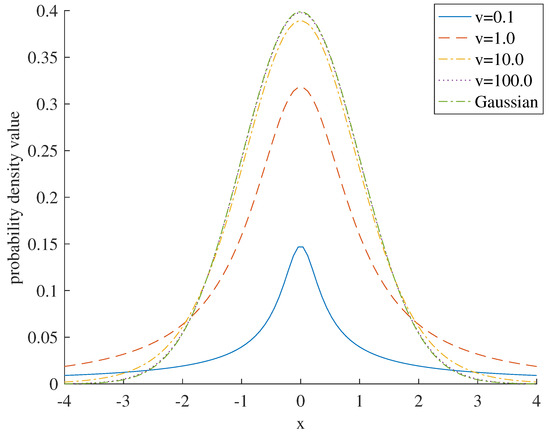
Figure 1.
Probability density of Student’s t-distribution of with different degrees of freedom.
Generalized to the multivariate Student’s t-distribution and using the same methodology as for the univariate variable [29,42], i.e.,
where is the dimension of and denotes the squared Mahalanobis distance, which is defined as follows:
The Student’s t-distribution is a formal generalization of the Gaussian distribution. When , the Student’s t-distribution can be simplified to a Gaussian distribution with a mean of and a precision of . Furthermore, the maximum likelihood parameter values of the Student’s t-distribution are more robust to outliers than other distributions.
3.2. Variational Inference
VI is a method for approximate inference of probabilistic model that approximates the true posterior distribution [43] by optimizing an easy-to-handle variational distribution , which is a family of distributions with parameters. VI transforms an inference problem into an optimization problem that minimizes the difference between the variational distribution and the true posterior distribution by adjusting the variational parameter , which is usually measured by the Kullback–Leibler () scattering measure [33,44].
sign
The scatter can be simplified to the following form:
Since , it follows that is a lower bound on the log-likelihood function , i.e., minimizing the scatter is equivalent to maximizing the evidence lower bound [45], it is common in VI to approximate the true posterior distribution by optimizing [46].
3.3. Markov Chain Monte Carlo
The fundamental principle of the MCMC is the construction of a Markov Chain for the purpose of approximating complex probability distribution [38,47]. A Markov Chain can be defined as a stochastic process in which the probability of a given state depends solely on the previous state and is independent of all preceding states. Monte Carlo, on the other hand, estimates numerical solutions by repeated random sampling. Among them, the Metropolis–Hastings algorithm is a representative algorithm for MCMC.
Assuming the state at time , the probability distribution to be sampled is , the Metropolis–Hastings algorithm [48] uses a Markov Chain with a transfer kernel :
where and are referred to as the suggestion distribution and acceptance distribution, respectively. is the transfer kernel of another Markov Chain and its probability value is not zero. A candidate state is randomly selected according to , while the acceptance probability is
Then the transfer kernel is
A number u is randomly selected from the interval (0,1) according to a uniform distribution, and if , it means accept and decided to transfer to state at moment i, i.e., ; otherwise, it means rejecting and deciding to stay in state x at moment i, i.e., state [49].
4. Methods
To overcome the influence of outliers and improve the classification accuracy of the model, a symplectic MCMC Student’s t-distribution hybrid regression model combining the flexibility of the hybrid model and the thick-tailed property of the Student’s t-distribution is constructed. The model can enhance the robustness of leptokurtic points in the data and improve classification accuracy by adjusting the number of components in the mixture model and the parameters of the Student’s t-distribution [50,51]. The hybrid model permits the capture of multiple distribution patterns of the data, and the properties of the t-distribution facilitate the accommodation of heavy-tailed distribution and outliers in the data, thereby ensuring the reliability of classification results despite the presence of outliers.
4.1. Mixed Student’s T-Distribution Regression Based on VI and MCMC (VMSTMR)
Assuming that x obeys the mixture distribution of K components, the Student’s t-distribution mixture model takes the form of
where the mixing coefficients , are the a priori probability values of the component with and for all k.
Assume that the input variables X and Y obey a linear relationship, i.e.,
where is the regression coefficient between and , is the measurement noise, and .
Therefore, it is possible to obtain
where and . When , it represents that belongs to the component, otherwise .
Since VI is an approximation method, there are inevitably some errors between the variational distribution it obtains and the true posterior distribution. This error may have an impact on the subsequent inference and classification accuracy, but the advantage of VI is that it improves computational efficiency. In contrast, the MCMC can approximate the true posterior distribution more accurately, but it has the disadvantage of requiring a longer running time to ensure that the sample distribution gradually approaches the true posterior distribution.
In Section 3.2, it is mentioned that the initial variational distribution is used to approximate the true posterior distribution . First, is optimized using VI. Then, is further improved by running an MCMC for a fixed number of iterations . Specifically, suppose that after several iterations of VI, is refined using an MCMC to obtain an approximation that is closer to the true posterior distribution, i.e.,
where is the overall transition kernel [52]. Since is an improvement of , is closer to than , i.e.,
The equality sign holds if and only if [53].
To eliminate , add a term to Equation (14), i.e.,
This scatter can be expressed as
As , converges to , and converges to the symmetric dispersion of the variational distribution with the posterior distribution.
4.2. Parameter Estimates
In the Bayesian framework, the original variational distribution is first parametrically evaluated using VI. The posterior probability is first calculated
The expectation for the intermediate variable
The expectation for the intermediate variable
Update weights
Updating the mean
Update precision
Updating the degrees of freedom
Updated regression coefficients
Update noise
This was followed by parameter optimization of the variational distribution using MCMC. The log-likelihood function was calculated for each data point
where is the mixing coefficient of the component, is the mean vector, is the precision vector, is the degrees of freedom, and is the observation.
where is the data dimension.
where is the probability density function of the Student’s t-distribution.
To avoid numerical overflow
The Metropolis–Hastings criterion decides whether to accept the new parameter values and calculate the acceptance probability
where is the probability of the new parameter and is the probability of the old parameter . A number u is randomly drawn from the interval (0,1) according to a uniform distribution with parameter if and parameter otherwise.
The HMC method proposes new parameter values
where is the Hamiltonian function, is the initial value, and is the proposed new parameter value. To ensure optimization of the HMC parameters, the step size must be adaptively adjusted according to the acceptance rate. If the acceptance rate is too low, the step size is reduced to 0.9 times the original acceptance rate, and if the acceptance rate is too high, the step size is increased to 1.1 times the original acceptance rate to explore the parameter space more efficiently. By continuously adjusting the step size, the goal is to stabilize the acceptance rate between approximately 0.65 and 0.75, which is the recommended acceptance rate range. The number of jump steps can also be adjusted if the step size has been adjusted to the appropriate range but the acceptance rate is still unsatisfactory. In the experiments, the number of jump steps will be adaptively adjusted according to the performance of the algorithm, and the strategy of adaptively adjusting the distribution of proposals will be used to improve the mixing efficiency of the Markov Chain, thus improving the overall performance of the algorithm.
After each iterative process is completed, the difference in the variational Bayesian MCMC is calculated, and the difference is compared with the specified threshold . When the difference is lower than , the algorithm is considered to have converged, i.e.,
When the difference is higher than , the algorithm proceeds to the next round of iterations if the number of iterations does not exceed the specified range.
4.3. Overall Flow of the Model
The classification process is divided into two phases: offline modeling and online prediction.
In the offline modeling phase, data such as cracker tube outlet temperature and tube inlet temperature are first collected from a petrochemical ethylene plant, the obtained data are cleaned, and the cleaned data are stored in a CSV file in the format of (samples, features) for subsequent processing. A VI is used to optimize a variational distribution to approximate the true posterior distribution. At the same time, Markov Chains are constructed using the MCMC to generate samples whose distribution will eventually converge to the true posterior. In the method of this paper, the variational distribution learned by VI is used as the initial distribution of the MCMC, the variational distribution is improved by iterating the specified number of rounds through the MCMC, and the parameters of VI are updated using the improved variational distribution. The offline modeling phase is completed when the VI and the MCMC are alternately iterated to the specified number of rounds or when the model converges.
In the online prediction phase, for the collected historical data, the values of its probability density function under the mixture components are calculated and the probability density of each mixture component is converted into a posteriori probabilities. By combining the features of the historical data with the a posteriori probabilities and multiplying them by a weight matrix, an output is obtained that represents the relative position of that data in each category. The category to which the data most likely belongs is determined by comparing the distance of the output to the category label. When the true value of the online analysis output is finally obtained, it is stored in the historical data. It can be used for continuous learning and improvement of the model. Offline modeling is carried out periodically or as needed to update the model. The hyperparameters are set to be the prior distribution of the model. The flowchart of VMSTMR is shown in Figure 2.
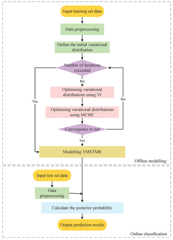
Figure 2.
Flowchart of VMSTMR.
Algorithm 1 gives the pseudo-code for the VMSTMR-based soft measurement model.
| Algorithm 1 Soft measurement model based on VMSTMR |
|
4.4. Evaluation Index
In this paper, a total of four model evaluation metrics are used, which are root mean square error (RMSE), accuracy (Accuracy), mean absolute error (MAE), and mean absolute percentage error (MAPE) [54,55]. Among them, RMSE is usually used to measure the accuracy of the model, which reflects the overall magnitude of the difference between the output values and the true values, where the smaller the value of RMSE, the better the classification effect of the model; Accuracy is usually used to assess the performance of the classification model, which reflects the ratio of the number of samples correctly classified by the model to the total number of samples, where the bigger the value of Accuracy, the better the classification performance of the model; MAE is usually used to measure the error of the model, which reflects the average of the error between the output value and the real value, where the smaller the value of MAE, the smaller the classification error of the model; MAPE is usually used to measure the performance of the model, which reflects the extent of the deviation between the output value and the real value expressed as a percentage, where the smaller the value of MAPE, the better the classification accuracy of the model. To summarize, RMSE, MAE, and MAPE are all indicators used to measure the classification error of the model, so the smaller the value, the better, indicating that the output result of the model is closer to the real value; meanwhile, Accuracy is an indicator used to measure the performance of the classification model, and the bigger the value, the better, indicating that the model is more capable of classification.
The formulas for the four evaluation metrics are as follows:
In the above equation, denotes the output value, y represents the true value, TP is the number of correctly categorized positive samples, TN is the number of correctly categorized negative samples, FP is the number of incorrectly categorized positive negative samples, FN is the number of incorrectly categorized negative positive samples, and m denotes the number of sample observations.
5. Results
In this experiment, PLSR [56], GPR [57], GMR [58], STMR [22], and SsSMM [32] are selected as benchmarks for the comparative analysis to evaluate the performance of different models by comparing the RMSE, Accuracy, MAE and MAPE values to estimate the performance of the different models.
To avoid the effect of initial parameter randomness, 50 simulations of PLSR, GPR, GMR, STMR, SsSMM, and VMSTMR algorithms were performed and averaged for each evaluation metric.
5.1. Simulation Experiments
Assuming the existence of a two-dimensional input variable and an output variable y, the input variables assume a mixed Gaussian distribution, and the specific parameter settings of the model are shown in Table 2.
Table 2.
Parameters of the three Gaussian distribution components.
A total of 2000 samples were randomly generated into three data sets, i.e., training, validation and test sets, each containing three categories, Model1, Model2 and Model3, and the sample ratio was distributed according to 6:2:2 to ensure that the training set contained 1200 samples and the test and validation sets contained 400 samples each. The training set is used to train the parameters of the VMSTMR model to be able to make an accurate classification of unseen data; the validation set is used to adjust the parameters of the VMSTMR model to avoid overfitting; and the test set is used to evaluate the final performance of the model after the model training is completed. The distribution of the noiseless data is shown in Figure 3.
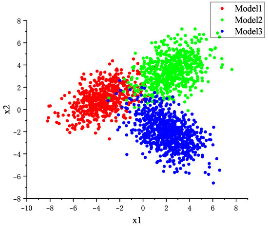
Figure 3.
Distribution of noise-free data.
To verify the robustness of the model, outlier points of 1%, 3%, 5%, and 7% were introduced in the input data samples. These outlier points are generated by transforming the eigenvalues of randomly selected sample data to values far from the center of their normal distribution. For example, introducing 1%, 3%, 5%, and 7% outlier points in a training set containing 2000 samples means adding 20 (1%), 60 (3%), 100 (5%), and 140 (7%) outlier points, respectively, to that data set. The distribution of the added random noise data is shown in Figure 4.
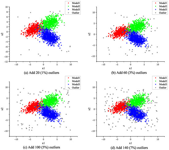
Figure 4.
Visualization of adding random noise data distribution.
To reduce random errors and improve the reliability of the results, a fixed random seed was used to ensure that the randomness remained consistent from one experiment to the next. The hyperparameters of the PLSR, GPR, GMR, STMR, SsSMM and VMSTMR models were then optimized using a grid search algorithm. After determining the optimal hyperparameters of the models, 50 repetitions of the simulation experiments were performed and a cross-validation technique was applied to increase the efficiency of data usage and reduce the chance of evaluation results. The evaluation metrics for each experiment were recorded in detail. In order to obtain a stable estimate of the model performance, the evaluation metrics of all experiments were averaged and the specific results of the obtained average performance metrics are shown in Table 3.
Table 3.
Mean values of each indicator for each model on randomized data.
By comparing the mean values of the indicators, it can be observed that the Accuracy of the PLSR model is the lowest regardless of whether outliers are added or not, or how many outliers are added, which indicates that it has the worst classification effect, and at the same time, the RMSE, MAE, and MAPE of the PLSR model are the largest, which indicates that it has the worst model performance. Comparatively, the Accuracy of the VMSTMR model is always the highest and provides the best classification effect. Its RMSE, MAE, and MAPE are the smallest, indicating the best model performance.
After calculation, it can be obtained that the RMSE of PLSR, GPR, GMR, STMR, and SsSMM models increased by 0.0571, 0.0650, 0.086, 0.0639, and 0.0511, respectively, and that of VMSTMR model only increased by 0.0049 when 1% outliers were added, which indicates that the classification accuracy of VMSTMR model in extreme cases is more stable and improved the dispersion of the error; the MAE of the VMSTMR model was reduced by 74.11%, 73.73%, 36.88%, 32.11%, and 28% compared to the PLSR, GPR, GMR, STMR, and SsSMM models, which significantly reduced the overall sample error; the MAPE was decreased by 72.62%, 70.37%, 12.76%, 32.17%, and 30.69% respectively, which indicates that the output values of the VMSTMR model deviate from the true values to a lesser extent during classification.
Similarly, the increase in RMSE as well as the relative degree of MAE and MAPE of each model after adding 3%, 5% and 7% outlier points were calculated, and it can be concluded that the VMSTMR model has the smallest increase in RMSE, which indicates that the VMSTMR model is more stable than the PLSR, GPR, GMR, STMR and SsSMM models in dealing with outlier points. At the same time, the relative increase in MAE and MAPE of the VMSTMR model is also the smallest, which means that the classification error of the VMSTMR model is relatively small when outliers are introduced, and the deviation between its classification results and the actual values is the smallest. Therefore, the VMSTMR model performs best in terms of robustness and its output results are closer to the real values.
The VMSMTR model combines VI and MCMC techniques to effectively overcome some of the limitations of the traditional model. Compared with PLSR, although PLSR can effectively deal with multicollinearity, it is not as flexible as the VMSMTR model in dealing with complex data distributions and outliers. The VMSMTR model is able to capture the diversity and complexity of the data more efficiently by mixing multiple Student’s t-distributions and is therefore more robust to outliers.
Compared to the GPR and GMR models, which use a Gaussian distribution as the base model, the VMSTMR model is less sensitive to outliers. This is because the VMSTMR model uses a mixture of multiple Student’s t-distributions, which allows it to adapt to non-Gaussian and multimodal data, thus improving the classification accuracy of the model.
Compared to the STMR and SsSMM models, the VMSTMR model achieves more stable parameter estimation by combining the VI and MCMC techniques, thus solving the approximation inaccuracy problem of the STMR and SsSMM models that can occur when a single VI technique is used to estimate model parameters. As a result, the VMSTMR model is able to capture the underlying distribution of the data more accurately and improve the generalization ability of the model.
The VMSTMR model excels at handling complex industrial data by combining VI and MCMC techniques, but this also leads to an increase in model run time. Specifically, the CPU execution time of the VMSTMR model is approximately one hundred and ten seconds. In contrast, PLSR, a linear regression method, is more computationally efficient with a CPU execution time of approximately seventy seconds. When dealing with large datasets, the CPU execution time of the GPR model increases significantly to approximately eighty seconds, and the CPU execution time of the GMR model is typically shorter than that of the VMSTMR model, which is approximately eighty-five seconds. Due to the omission of the MCMC step, the STMR model has a shorter CPU execution time than the VMSTMR model, approximately ninety seconds. The SsSMM model has a similar CPU execution time to the VMSTMR model, approximately one hundred seconds, when processing both labeled and unlabeled data.
5.2. Actual Industrial Data
Actual operating data from an ethylene cracker at a major petrochemical company are used in this section. When screening the characteristics, the experience of local experts and the mechanism model of catalytic cracking are combined. Finally, six key characteristics are selected, including the furnace tube outlet temperature, the furnace tube inlet temperature, the adiabatic pressure ratio, the cross-section pressure, and the venturi pressure, and the framework of the diagnostic reasoning system for the coking of the furnace tube of an ethylene cracking furnace tube is shown in Figure 5. In addition, the furnace tube coking condition is categorized into four normal levels mild coking, moderate coking and severe coking, according to the degree of furnace tube coking.
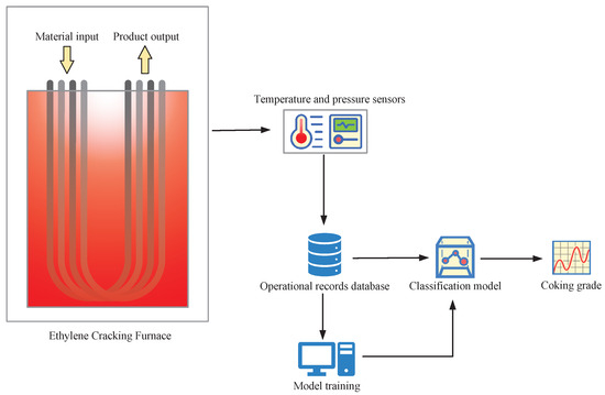
Figure 5.
Framework of coking diagnostic inference system.
As the unprocessed output of the model is a floating-point value and the coking level of the furnace tube is an integer value, the output of the model is processed as follows in order to enable the model to more accurately predict the coking level of the furnace tube.
where is the degree of coking in the furnace tube, is the output of the unprocessed model, and is the processed output.
The dataset used in this section contains 5000 samples, of which the training set accounts for 3500 samples and the test set accounts for 1500 samples. RMSE, Accuracy, MAE, and MAPE are used as evaluation metrics to measure the prediction accuracy and robustness of each model.
A large number of iterations were performed to ensure that the MCMC chain could adequately mix and explore the parameter space. At the same time, an algorithm for adaptively adjusting the proposal distribution was used to improve the mixing efficiency of the chain. Under this configuration, the acceptance rate during MCMC iterations was stabilized at around 0.7, which is in the ideal acceptance rate interval and helps to maintain the efficiency and exploratory power of the algorithm. The variation in the acceptance rate during MCMC iterations is shown in Figure 6.
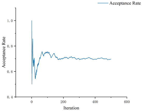
Figure 6.
Framework of coking diagnostic inference system.
Table 4 demonstrates the average values of the evaluated metrics, and according to the computational analysis, it can be concluded that the VMSTMR model exhibits superior performance compared to the PLSR, GPR, GMR, STMR, and SsSMM models in all cases, regardless of whether or not outliers are introduced or how the number of outliers varies.
Table 4.
Average values of each indicator for each model on industrial data.
Based on the experimental results in Table 4, it can be seen that the VMSTMR model performs best, followed by the SsSMM model. Further, by looking at Figure 7, it can be found that in Figure 7a, the overlap between the true and output values of the VMSTMR model is lower than that in Figure 7b. Therefore, it can be concluded that the VMSTMR model is better than the SsSMM model for good classification, i.e., the VMSTMR model performs the best in terms of classification effectiveness.
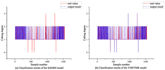
Figure 7.
Classification results of each model on industrial data.
In order to better evaluate the performance of the VMSTMR model and to explore different variants of the MCMC kernel function to improve its sampling efficiency, uniform kernels, Gaussian kernels and Laplacian kernels were first compared, and then the effectiveness of the Random Walk Metropolis(RWM) as an alternative proposal kernel was tested. A 0% data set was used in the experiments for testing. The test results show that the RMSE, Accuracy, MAE and MAPE of uniform kernels are 0.2001, 0.9596, 0.0404 and 1.7524, respectively, the RMSE, Accuracy, MAE and MAPE of Gaussian kernels are 0.1804, 0.9675, 0.0326 and 1.621, respectively. The RMSE, Accuracy, MAE and MAPE of the Laplacian kernels are 0.2165, 0.9531, 0.0469 and 2.2193, respectively. Compared to the VMSTMR model, there is a time saving of approximately twenty to forty seconds for both the uniform, Gaussian and Laplacian kernels. However, this time advantage did not translate into improved experimental results, i.e., although sampling speed was improved, accuracy and reliability were sacrificed. To further validate the optimality of the adopted method, the RWM method was parameterized and tested as an alternative proposal kernel. The test results show that the performance of the parametrically tuned RWM on the four metrics of RMSE, Accuracy, MAE and MAPE are 0.215, 0.9538, 0.0462 and 4.4278, respectively. Despite the parametric tuning, RWM still falls short of VMRM on the three performance metrics of RMSE, MAE and MAPE. This suggests that although the uniform, Gaussian and Laplace kernels have advantages in sampling efficiency, these kernels and the RWM do not perform as well as the VMSTMR model in terms of accuracy and reliability. Therefore, the proposed kernel selected for the VMSTMR model is a more appropriate choice for the application of ethylene coke diagnosis.
6. Conclusions
This paper addresses the limitations of traditional ethylene cracker furnace tube coking diagnostic methods in terms of detection period, accuracy and real-time, as well as the multimodal, nonlinear, non-Gaussian and strong noise problems of the production process data. To this end, a novel soft measurement method is proposed: the mixed Student’s t-distribution regression soft measurement model based on VI and MCMC. In order to assess the reliability of VMSTMR, outlier points at 1%, 3%, 5% and 7% were incorporated into the experimental data set. The experimental results demonstrate that while the classification performance of all methods declines with an increase in the proportion of outlier points, VMSTMR exhibits a relatively lower decline. VMSTMR outperforms the PLSR, GPR, GMR, STMR and SsSMM methods in classifying the coking situation of ethylene cracker tubes, indicating that VMSTMR possesses a high level of robustness in the presence of outliers.
In actual industrial production, the application of the VMSTMR model can realize real-time monitoring of the coking condition of the ethylene cracker furnace tube. This is of great significance for optimizing the production process, reducing equipment downtime and extending the service life of the furnace tube, which in turn improves the production efficiency of ethylene and the economic benefits of the enterprise. Therefore, the introduction of the VMSTMR model can not only become a key technology for intelligent maintenance and fault prediction of ethylene crackers but is also expected to promote the technological progress and sustainable development of the entire petrochemical industry.
7. Future Research Directions
In machine learning and statistics, nonlinear data processing is the handling of nonlinear relationships between variables, which includes techniques such as data transformation, nonlinear model application, and feature engineering. For example, in support vector machines (SVMs), the choice of kernel function is critical in dealing with nonlinear problems. Commonly used kernel functions include linear kernel, polynomial kernel, radial basis function (RBF) kernel, and sigmoid kernel, etc., and their choice depends on the data characteristics and the specific needs of the problem. In addition, a hybrid model improves model performance by combining the advantages of different models, but this may also increase the complexity and training difficulty of the model.
Despite the significant achievements of the VMSTMR model in improving robustness, it still faces challenges in dealing with nonlinear data. To further improve the VMSTMR model’s ability to handle nonlinear data, future research will focus on addressing the model’s limitations in this area. Specifically, the research will explore the introduction of stacked self-encoders to deal with nonlinear problems. The stacked self-encoder is able to map raw data to a feature space that better reflects its intrinsic structure and complex relationships through a multilayer nonlinear transformation. This approach first learns an efficient representation of the data through layer-by-layer pre-training, and then optimizes the entire network through global fine-tuning to capture the complex nonlinear relationships in the data. This strategy not only improves the classification accuracy and generalization ability of the VMSTMR model in complex industrial data environments but also increases the robustness and applicability of the model.
Author Contributions
Q.L. was responsible for the overall idea of this paper, Z.P. and J.H. were responsible for the algorithm design, D.C. and C.L. were responsible for the experiments and result analysis. This paper was written by C.L. All authors have read and agreed to the published version of the manuscript.
Funding
The work presented in this paper was supported by: National Natural Science Foundation of China (62273109); Guangdong Basic and Applied Basic Research Foundation (2022A1515012022, 2023A1515240020, 2023A1515011913); Key Field Special Project of Department of Education of Guangdong Province (2024ZDZX1034); Key Realm R&D Program of Guangdong Province (2021B0707010003); Maoming Science and Technology Project (2022DZXHT028, 210429094551175, mmkj2020033); Projects of PhDs’ Start-up Research of GDUPT (XJ2022000301, 2023bsqd1002, 2023bsqd1013).
Data Availability Statement
The data presented in this study are available on request from the corresponding author due to privacy.
Conflicts of Interest
The authors declare no conflicts of interest. The funders had no role in the design of the study; in the collection, analyses, or interpretation of data; in the writing of the manuscript; or in the decision to publish the results.
Abbreviations
The following abbreviations are used in this manuscript:
| AI | Artificial intelligence |
| GAN | Generative adversarial network |
| GMR | Gaussian Mixture Regression |
| GPR | Gaussian Process Regression |
| GRU | Gated recurrent unit |
| LSTM-DeepFM | The Long Short-Term Memory–Deep Factorization Machine |
| MAE | Mean absolute error |
| MAPE | Mean absolute percentage error |
| MCMC | Markov Chain Monte Carlo |
| PLSR | Partial Least Squares Regression |
| RMSE | Root mean square error |
| SsSMM | Semi-supervised robust modeling method |
| STMR | Bayesian Student’s T-Distribution Mixture Regression |
| VAE | Variational autoencoder |
| VBGMR | Variational Bayesian Gaussian mixture regression |
| VBMC | Variational Bayesian Monte Carlo |
| VBSMR | Variational Bayesian Mixed Student’s t-distribution Regression |
| VI | Variational Inference |
| VM | Variational Bayesian Markov Chain Monte Carlo |
| VMSTMR | Variational Bayesian MCMC mixed Student’s t-distribution regression |
References
- Zhao, J.; Peng, Z.; Cui, D.; Li, Q.; He, J.; Qiu, J. A method for measuring tube metal temperature of ethylene cracking furnace tubes based on machine learning and neural network. IEEE Access 2019, 7, 158643–158654. [Google Scholar] [CrossRef]
- Peng, Z.; Zhao, J.; Yin, Z.; Gu, Y.; Qiu, J.; Cui, D. ABC-ANFIS-CTF: A method for diagnosis and prediction of coking degree of ethylene cracking furnace tube. Processes 2019, 7, 909. [Google Scholar] [CrossRef]
- Shu, L.; Mukherjee, M.; Pecht, M.; Crespi, N.; Han, S.N. Challenges and research issues of data management in IoT for large-scale petrochemical plants. IEEE Syst. J. 2017, 12, 2509–2523. [Google Scholar] [CrossRef]
- Maoxuan, Z. Simulation of burning process in cracking furnace of ethylene plant. Ethyl. Ind. 2020, 32, 34–37+5. [Google Scholar]
- Xiaona, H. The Simulation of Ethylene Cracking Furnace Decking Process, Its Application and Optimal Control; Beijing University of Chemical Technology: Beijing, China, 2013. [Google Scholar]
- Shanhai, X. The Simulation and Control of Decoking Process of Ethylene Cracking Furnace; Beijing University of Chemical Technology: Beijing, China, 2016. [Google Scholar]
- Wen, Z.; Qian, B.; Hu, R.; Jin, H.; Yang, Y. Ethylene yield prediction based on bi-directional GRU optimized by learning-based artificial bee colony algorithm. Control Theory Appl. 2023, 40, 1746–1756. [Google Scholar]
- Yuan, X.; Ou, C.; Wang, Y.; Yang, C.; Gui, W. A layer-wise data augmentation strategy for deep learning networks and its soft sensor application in an industrial hydrocracking process. IEEE Trans. Neural Netw. Learn. Syst. 2019, 32, 3296–3305. [Google Scholar] [CrossRef]
- Brunner, V.; Siegl, M.; Geier, D.; Becker, T. Challenges in the development of soft sensors for bioprocesses: A critical review. Front. Bioeng. Biotechnol. 2021, 9, 722202. [Google Scholar] [CrossRef]
- Jiang, Y.; Yin, S.; Dong, J.; Kaynak, O. A review on soft sensors for monitoring, control, and optimization of industrial processes. IEEE Sens. J. 2020, 21, 12868–12881. [Google Scholar] [CrossRef]
- Sun, Q.; Ge, Z. A survey on deep learning for data-driven soft sensors. IEEE Trans. Ind. Inform. 2021, 17, 5853–5866. [Google Scholar] [CrossRef]
- Yuan, X.; Li, L.; Shardt, Y.; Wang, Y.; Yang, C. Deep learning with spatiotemporal attention-based LSTM for industrial soft sensor model development. IEEE Trans. Ind. Electron. 2020, 68, 4404–4414. [Google Scholar] [CrossRef]
- Sun, H.; Hu, T.; Ma, Y.; Liu, Z.; Liang, C. Study on Soft Sensing Technology of Gas Pipeline Compressor Flow Based on Random Fores. Autom. Petro-Chem. Ind. 2024, 60, 21–24. [Google Scholar]
- Cao, P.; Luo, X. Modeling of soft sensor for chemical process. CIESC J. 2013, 64, 788–800. [Google Scholar]
- Wang, J. Bayesian Mixture Model-Based Robust Soft Sensor Modeling and Application. Master’s Thesis, Zhejiang University, Hangzhou, China, 2022. [Google Scholar]
- Zhao, J. Study on Intelligent Coking Diagnosis Method of Ethylene Cracking Furnace Tubs. Master’s Thesis, Guangdong University of Technology, Guangzhou, China, 2020. [Google Scholar]
- Zhu, J.; Ge, Z.; Song, Z. Variational Bayesian Gaussian mixture regression for soft sensing key variables in non-Gaussian industrial processes. IEEE Trans. Control Syst. Technol. 2016, 25, 1092–1099. [Google Scholar] [CrossRef]
- Qin, Y.; Liu, X.; Yue, C.; Wang, L.; Gu, H. A tool wear monitoring method based on data-driven and physical output. Robot. Comput.-Integr. Manuf. 2025, 91, 102820. [Google Scholar] [CrossRef]
- Ren, L.; Wang, T.; Laili, Y.; Zhang, L. A data-driven self-supervised LSTM-DeepFM model for industrial soft sensor. IEEE Trans. Ind. Inform. 2021, 18, 5859–5869. [Google Scholar] [CrossRef]
- Zhang, C.; Bütepage, J.; Kjellström, H.; Mandt, S. Advances in variational inference. IEEE Trans. Pattern Anal. Mach. Intell. 2018, 41, 2008–2026. [Google Scholar] [CrossRef]
- Xie, F.; Shen, Y. Bayesian estimation for stochastic volatility model with jumps, leverage effect and generalized hyperbolic skew Student’s t-distribution. Commun. Stat.-Simul. Comput. 2023, 52, 3420–3437. [Google Scholar] [CrossRef]
- Xia, C.; Peng, Z.; Cui, D.; Li, Q.; Sun, L. Concentration Diagnosis in Soft Sensing Based on Bayesian T-Distribution Mixture Regression. In Proceedings of the FSDM 2023, Chongqing, China, 10–13 November 2023; pp. 362–371. [Google Scholar]
- Zhai, X. Momentum-Based Monte Carlo Method for Stochastic Gradient Martensitic Chains. Master’s Thesis, Shanghai Normal University, Shanghai, China, 2023. [Google Scholar]
- Hirt, M.; Kreouzis, V.; Dellaportas, P. Learning variational autoencoders via MCMC speed measures. Stat. Comput. 2024, 34, 164. [Google Scholar] [CrossRef]
- Jiang, H.; Liu, Y.; He, S.; Luo, J.; Xu, T. A Study on Mechanistic Prediction Model of Gathering Pipelines in CO2 Environment. J. Southwest Pet. Univ. (Sci. Technol. Ed.) 2023, 45, 178–188. [Google Scholar]
- Wang, S.; Tian, W.; Li, C.; Cui, Z.; Liu, B. Mechanism-based deep learning for tray efficiency soft-sensing in distillation process. Reliab. Eng. Syst. Saf. 2023, 231, 109012. [Google Scholar] [CrossRef]
- Guo, R.; Liu, H. A hybrid mechanism-and data-driven soft sensor based on the generative adversarial network and gated recurrent unit. IEEE Sens. J. 2021, 21, 25901–25911. [Google Scholar] [CrossRef]
- He, Z.; Qian, J.; Li, J.; Hong, M.; Man, Y. Data-driven soft sensors of papermaking process and its application to cleaner production with multi-objective optimization. J. Clean. Prod. 2022, 372, 133803. [Google Scholar] [CrossRef]
- Svensén, M.; Bishop, C. Robust Bayesian mixture modelling. Neurocomputing 2005, 64, 235–252. [Google Scholar] [CrossRef]
- Wang, J.; Shao, W.; Song, Z. Student’s-t mixture regression-based robust soft sensor development for multimode industrial processes. Sensors 2018, 18, 3968. [Google Scholar] [CrossRef] [PubMed]
- Yang, L.; Tian, Z.; Wen, J.; Yan, W. Variational Bayesian-based adaptive non-rigid point set matching. J. Northwest. Polytech. Univ. 2018, 36, 942–948. [Google Scholar] [CrossRef]
- Shao, W.; Ge, Z.; Song, Z.; Wang, J. Semisupervised robust modeling of multimode industrial processes for quality variable prediction based on student’s t mixture model. IEEE Trans. Ind. Inform. 2019, 16, 2965–2976. [Google Scholar] [CrossRef]
- Acerbi, L. Variational bayesian monte carlo. Adv. Neural Inf. Process. Syst. 2018, 31, 8222–8232. [Google Scholar]
- Wang, J.; Shao, W.; Song, Z. Robust inferential sensor development based on variational Bayesian Student’st mixture regression. Neurocomputing 2019, 369, 11–28. [Google Scholar] [CrossRef]
- De Figueiredo, L.P.; Grana, D.; Roisenberg, M.; Rodrigues, B. Gaussian mixture Markov chain Monte Carlo method for linear seismic inversion. Geophysics 2019, 84, R463–R476. [Google Scholar] [CrossRef]
- Wiese, J.; Wimmer, L.; Papamarkou, T.; Bischl, B.; Günnemann, S.; Rügamer, D. Towards efficient MCMC sampling in Bayesian neural networks by exploiting symmetry. In Proceedings of the Joint European Conference on Machine Learning and Knowledge Discovery in Databases 2023, Turin, Italy, 18–22 September 2023; Springer Nature: Cham, Switzerland, 2023; pp. 459–474. [Google Scholar]
- Chandra, R.; Simmons, J. Bayesian neural networks via MCMC: A python-based tutorial. arXiv 2023, arXiv:2304.02595. [Google Scholar] [CrossRef]
- Yi, Z.; Wei, Y.; Cheng, C.; He, K.; Sui, Y. Improving sample efficiency of high dimensional Bayesian optimization with MCMC. arXiv 2024, arXiv:2401.02650. [Google Scholar]
- Bishop, C. Pattern Recognition and Machine Learning; Springer: New York, NY, USA, 2006. [Google Scholar]
- Galarza, C.; Lin, T.; Wang, W.; Lachos, V. On moments of folded and truncated multivariate Student-t distributions based on recurrence relations. Metrika 2021, 84, 825–850. [Google Scholar] [CrossRef]
- Virolainen, S. A mixture autoregressive model based on Gaussian and Student’st-distributions. Stud. Nonlinear Dyn. Econom. 2022, 26, 559–580. [Google Scholar]
- Lambert, M.; Chewi, S.; Bach, F.; Bonnabel, S.; Rigollet, P. Variational inference via Wasserstein gradient flows. Adv. Neural Inf. Process. Syst. 2022, 35, 14434–14447. [Google Scholar]
- Dhaka, A.; Catalina, A.; Welandawe, M.; Andersen, M.; Huggins, J.; Vehtari, A. Challenges and opportunities in high dimensional variational inference. Adv. Neural Inf. Process. Syst. 2021, 34, 7787–7798. [Google Scholar]
- Cao, Y.; Jan, N.; Huang, B.; Fang, M.; Wang, Y.; Gui, W. Multimodal process monitoring based on variational Bayesian PCA and Kullback–Leibler divergence between mixture models. Chemom. Intell. Lab. Syst. 2021, 210, 104230. [Google Scholar] [CrossRef]
- Blei, D.; Kucukelbir, A.; McAuliffe, D. Variational inference: A review for statisticians. J. Am. Stat. Assoc. 2017, 112, 859–877. [Google Scholar] [CrossRef]
- Chen, X. Research on Adaptive Variational Contrastive Divergence. Master’s Thesis, Xiamen University, Xiamen, China, 2020. [Google Scholar]
- Benedetti, M.; Coyle, B.; Fiorentini, M.; Lubasch, M.; Rosenkranz, M. Variational inference with a quantum computer. Phys. Rev. Appl. 2021, 16, 044057. [Google Scholar] [CrossRef]
- Hang, L. Statistical Learning Method, 2nd ed.; Tsinghua University Press: Beijing, China, 2012. [Google Scholar]
- Ashton, G.; Talbot, C. Bilby-MCMC: An MCMC sampler for gravitational-wave inference. Mon. Not. R. Astron. Soc. 2021, 507, 2037–2051. [Google Scholar] [CrossRef]
- Ilboudo, W.; Kobayashi, T.; Sugimoto, K. Robust stochastic gradient descent with student-t distribution based first-order momentum. IEEE Trans. Neural Netw. Learn. Syst. 2020, 33, 1324–1337. [Google Scholar] [CrossRef]
- Zhuang, J.; Jing, X.; Jia, X. Mining negative samples on contrastive learning via curricular weighting strategy. Inf. Sci. 2024, 668, 120534. [Google Scholar] [CrossRef]
- Ruiz, F.; Titsias, M. A contrastive divergence for combining variational inference and MCMC. In Proceedings of the International Conference on Machine Learning 2019, Long Beach, CA, USA, 10–15 June 2019; Long Beach Convention Center: Long Beach, CA, USA, 2019; pp. 5537–5545. [Google Scholar]
- Nguyen, Q.; Low, B.; Jaillet, P. Variational bayesian unlearning. Adv. Neural Inf. Process. Syst. 2020, 33, 16025–16036. [Google Scholar]
- Yan, L.; Wang, Z. Multi-step predictive soft sensor modeling based on STA-BiLSTM-LightGBM combined model. CIESC J. 2023, 74, 3407–3418. [Google Scholar]
- Lai, X.; Zhu, G.; Chambers, J. A fuzzy adaptive extended Kalman filter exploiting the Student’st distribution for mobile robot tracking. Meas. Sci. Technol. 2021, 32, 105017. [Google Scholar] [CrossRef]
- Burnett, A.C.; Anderson, J.; Davidson, K.J.; Ely, K.S.; Lamour, J.; Li, Q.; Morrison, B.D.; Yang, D.; Rogers, A.; Serbin, S.P. A best-practice guide to predicting plant traits from leaf-level hyperspectral data using partial least squares regression. J. Exp. Bot. 2021, 72, 6175–6189. [Google Scholar] [CrossRef] [PubMed]
- Ebden, M. Gaussian Processes for Regression: A Quick Introduction; The Website of Robotics Research Group in Department on Engineering Science, University of Oxford: Oxford, UK, 2008. [Google Scholar] [CrossRef]
- Sepúlveda, A.; Guido, R.; Castellanos-Dominguez, G. Estimation of relevant time–frequency features using Kendall coefficient for articulator position inference. Speech Commun. 2013, 55, 99–110. [Google Scholar] [CrossRef]
Disclaimer/Publisher’s Note: The statements, opinions and data contained in all publications are solely those of the individual author(s) and contributor(s) and not of MDPI and/or the editor(s). MDPI and/or the editor(s) disclaim responsibility for any injury to people or property resulting from any ideas, methods, instructions or products referred to in the content. |
© 2025 by the authors. Licensee MDPI, Basel, Switzerland. This article is an open access article distributed under the terms and conditions of the Creative Commons Attribution (CC BY) license (https://creativecommons.org/licenses/by/4.0/).