Abstract
Seasonal and industrial fluctuations in natural gas demands require optimized gas storage operations, especially in depleted reservoirs, to ensure a stable supply. This study proposes a novel optimization model for injection–production processes using the simulated annealing–particle swarm optimization (SA-PSO) algorithm. The model focuses on minimizing pressure variances across different reservoir blocks during injection–production cycles. The approach is applied to the W23 underground gas storage facility, where a high-precision 3D geological model and numerical simulations were developed. The SA-PSO algorithm effectively reduced pressure differentials during the sixth injection–production cycle, improving reservoir efficiency. During the gas injection period, the optimized pressure difference between blocks was reduced to one-eighth of that in the initial plan. The average formation pressures in Phase I and Phase II decreased by 0.35 MPa and 0.76 MPa, respectively. During the gas production period, the optimized pressure difference between blocks was reduced to one-tenth of that in the initial plan. The average formation pressures in Phase I and Phase II increased by 0.4 MPa and 1.21 MPa, respectively. The optimized injection–production strategy enhances working gas capacity, maintains balanced formation pressures, and mitigates risks such as high pressure and salt precipitation. The findings demonstrate the potential of SA-PSO optimization to improve the operational efficiency and safety of gas storage reservoirs.
1. Introduction
Natural gas, recognized for its environmental advantages, economic efficiency, and high energy density, plays a pivotal role in both residential and industrial applications [1]. However, fluctuations in the supply and demand of natural gas, propelled by factors like climate variations, industrial expansion, and evolving consumption patterns, pose challenges to the traditional methods of gas gathering and transportation. These traditional methods are becoming increasingly insufficient in guaranteeing a balanced supply [2].
Conventional peak load regulation measures for natural gas encompass underground gas storage (UGS), liquefied natural gas (LNG) receiving stations, and gas field adjustment [3,4]. The LNG receiving station adjustment has weak risk resistance. External factors like inconsistent supply sources, fluctuating transportation costs due to oil prices and tariffs, and adverse weather disrupt operations. Gas field adjustment mainly uses super intensive extraction and increasing pressure difference. Both can cause severe damage, such as rapid reserve depletion and land subsidence, threatening long-term gas field operation. In contrast to other load regulating techniques, UGS boasts several remarkable merits. It can store large volumes of gas, has a wide regulatory scope for various demand changes, and incurs low operating costs [5,6]. UGS not only solves seasonal demand imbalance by storing and releasing gas as needed, but also has strategic significance in enhancing energy security and reducing import dependence [7].
UGS using depleted gas reservoirs is crucial for managing seasonal gas demand variations [8]. These reservoirs, often repurposed due to their infrastructure and containment capabilities, serve as strategic reserves for peak shaving and emergency supply [9]. The optimization of gas storage operations has become a key area of research and industry interest.
In recent years, efforts to improve injection and production efficiency in gas storage have shifted from empirical methods and simplified models to mathematical modeling and numerical simulations [10]. These methods better address the complexities of large-scale UGS systems, offering more accurate optimization strategies for injection and withdrawal processes. Numerical simulations enhance our understanding of reservoir dynamics, aiding in resource recovery and long-term planning [11].
A conventional methodology for optimizing injection–production schemes involves the utilization of numerical simulation to develop reservoir models. Bagci et al. (2007) [12] employed a black oil model to simulate and evaluate the feasibility of new horizontal wells designated as injection–production wells in depleted gas reservoirs intended for storage purposes. Turryen et al. (2000) [13] utilized material balance diagram and productivity equation to simulate the performance of gas storage, including a good layout, the number of horizontal wells, lateral length, and completion skin, while investigating their effects on gas storage operations. B. Moradi et al. (2009) [14] simulated the impact of injection–production cycles on rock properties and condensate, demonstrating that an increase in cycles leads to a reduction in condensate within the near-well area, thereby enhancing gas-phase permeability. Subbiah et al. (2008) [15] developed a geodynamics model to assess geological structures, formation pressure, rock strength, and sand stability, ultimately recommending completion strategies to ensure stable injection–production operations. Ponomareva et al. (2022) [16] conducted a multidimensional analysis of actual reservoir data to integrate operational, geological, and reservoir characteristics into a predictive model for formation pressure.
Numerical simulation facilitates the accurate modeling of reservoir flow and the optimization of production processes. However, traditional simulation software frequently encounters low optimization efficiency due to the multitude of influencing factors and inherent complexity. With the rapid advancements in mathematical modeling and machine learning, an increasing number of researchers are employing these methodologies to enhance the optimization of gas storage injection and production [17]. Evolutionary algorithms, such as the genetic algorithm (GA) [18], particle swarm optimization (PSO) [19], artificial bee colony (ABC) [20], differential evolution (DE) [21], and simulated annealing (SA) [22], offer effective methods for parameter optimization.
Wu et al. (2020) [23] proposed the utilization of neural networks as an alternative to numerical simulations for predicting the distribution of remaining oil. This approach was integrated with a gradient-free differential evolution algorithm to optimize injection and production parameters, employing net present values (NPVs) as the objective function. Fadilah et al. (2019) [24] implemented a Gbest-guided artificial bee colony algorithm to model the relationship between injection and production to maximize the mathematical model. Farahi et al. (2022) [25] employed an adapted multi-objective particle swarm optimization (MOPSO) algorithm to achieve a balance between long-term and short-term net present values (LNPVs and SNPVs) along the Pareto front, facilitating optimized decision-making. Azamipour et al. (2018) [26] utilized a combination of genetic algorithms (GAs) and multi-body search techniques to maximize the NPVs, thereby optimizing production rates and water injection to enhance reservoir recovery.
Compared to genetic algorithms, PSO has a unique feature: the particles retain memory. In PSO, information is shared only by the globally best particle, unlike genetic algorithms where chromosomes exchange information among themselves. This results in less information exchange in PSO, with updates focused solely on the global optimal solution [27]. PSO’s operational rules are simpler, often leading to faster convergence to the optimal solution. Additionally, it is easy to implement, requires fewer parameters, and has a quick convergence rate, making it effective for complex optimization tasks in petroleum engineering [28]. However, the update position constraints of the particles are less and degradation problems may occur, so the SA algorithm is introduced to enhance the quality of the position update and the enhanced algorithm obtains a stronger global search capability after combining the SA algorithm with the PSO algorithm.
Therefore, this study proposes an injection–production optimization model based on SA-PSO to enhance the operational scheme of large, depleted gas storage facilities. Initially, a comprehensive analysis of the geological characteristics and reservoir properties of the W23 gas storage facility is presented. Utilizing measured data and numerical simulations, a high-precision three-dimensional geological model and a corresponding numerical simulation model have been developed, establishing a robust foundation for the subsequent optimization scheme. Subsequently, this paper addresses the limitations of existing injection and production schemes by validating the model’s reliability through historical matching. Large, depleted gas storage facilities typically consist of multiple injection–production blocks. During the production process, the formation pressures of each block vary differently with the changes in the injected and produced gas volumes, making it extremely easy to form formation pressure differences between blocks [29]. Excessively high formation pressure differences between blocks may lead to the damage of fault sealing, resulting in gas channeling or leakage accidents [30]. To ensure the long-term safe and stable operation of the gas storage facility, this paper applies the SA-PSO algorithm to optimize the injection and production volumes in the sixth injection–production cycle. The objective is to minimize the pressure differences between blocks, and the injection and production volumes of each block are redistributed. Finally, a comparative analysis with conventional injection–production schemes illustrates the advantages of the optimized approach in practical applications, demonstrating its effectiveness in enhancing working gas volume and balancing pressure differentials between blocks. In conclusion, this study not only introduces a novel methodology for the injection–production optimization of large, depleted gas storage reservoirs but also serves as a valuable reference for future research in this domain.
2. Materials and Methods
2.1. Optimization Model of Injection–Production
In the context of injection–production operations within large, depleted gas reservoir storage, it is crucial to formulate effective well-opening strategies and to determine individual good injection and production rates across various periods and zones. This process necessitates the definition of objective functions, constraints, and decision variables pertinent to optimization models for injection and production. As storage capacities continue to increase, the maximization of reservoir capacity and peak-shaving capabilities demands a simulation-based methodology that incorporates multiple factors to develop efficient injection–production plans. By synthesizing operational conditions and creating optimization algorithms within established constraints, this approach significantly enhances the practical application for on-site analysis and informed decision-making.
Balancing the pressure differences between blocks also depends on the reservoir properties of each block. Therefore, during the optimization process, the property differences in each block need to be taken into account. Regarding permeability, a high-permeability reservoir allows good fluid flow and rapid pressure transmission, while a low-permeability one does the opposite, easily leading to pressure differences. In blocks with high porosity, more fluids can be stored and pressure changes slowly, whereas, in those with low porosity, the situation is reversed. In terms of fluid saturation, high natural gas saturation results in significant pressure changes during injection and production, and high oil and water saturation hinders gas flow and pressure transmission.
2.1.1. Objective Function
To ensure the long-term, stable operation of large, depleted gas reservoir storage, optimization research is conducted with the goal of maintaining balanced formation pressure changes across the storage area. Statistically, variance represents the difference between individual samples and the overall average, reflecting the degree of deviation or dispersion. Thus, inter-block formation pressure variance indicates the pressure deviation among blocks. Minimizing this variance, particularly post-injection, helps achieve balanced pressure across the storage. The objective function of the injection optimization model minimizes inter-block pressure variance, with a similar approach used for production optimization, reversing the flow direction. The expression is as follows:
where f represents the inter-block formation pressure variance, MPa2; N is the total number of injection blocks in the gas storage reservoir; denotes the total number of time periods; j represents the number of injection and production blocks, j ∈ N; t is the injection and production time period, t ∈ tmax; is the pressure of jth block in tth period, MPa; and is the average pressure of all blocks in tth period, MPa.
2.1.2. Constraints
- Total gas injection volume constraint for UGS
In the gas injection process of a storage reservoir, the cumulative injection volumes across all blocks must meet the total injection volume requirement for the entire storage facility, as delineated in Equation (2). When the injection demands surpass the facility’s capacity, the effectiveness of the optimization process is significantly reduced. Furthermore, it is noteworthy that within a given block, the individual well productivity equations and injection capacities exhibit minimal variation.
where represents the total gas injection volume for the gas storage facility during the tth period, 104 m3/d; is the number of production days in the tth period, d; and is the total daily gas injection volume for the jth block during the tth period, 104 m3/d.
- 2.
- Maximum well injection volume constraint
In each block, the injection rate for individual wells is limited by their maximum injection capacity, as delineated in Equation (3). This process mainly consists of two sub-processes: gas flows from the wellhead to the bottom of the vertical injection–production well, overcoming pipeline frictional resistance; then, it flows from the well bottom into the reservoir, overcoming reservoir resistance. Therefore, the gas injection rate of a single well is mainly determined by the wellhead pressure and the reservoir pressure. By solving the vertical pipe flow equation (Equation (4)) and the stable seepage equation of the reservoir (Equation (6)), the gas injection rate of a single well under specific wellhead and reservoir pressures can be obtained [31].
Regarding the two parameters determining the single-well gas injection rate, the reservoir pressure cannot be artificially altered, but the wellhead pressure can be adjusted by changing the operating parameters of the surface compressor unit. Thus, the maximum gas injection rate of a single well can be achieved when the wellhead pressure reaches its maximum.
where is the maximum daily injection volume for a single well in block j, 104 m3/d; Pwf is the bottom-hole pressure, Mpa; Pwh is the tubing wellhead pressure, Mpa; λ is the tubing resistance coefficient; T is the average temperature of moving gas in the wellbore, K; Z is the average deviation factor of moving gas in the wellbore; d is the tubing inner diameter, cm; is the relative density of natural gas; H is the midpoint depth of the gas layer, m; P is the formation pressure, Mpa; is the injection volume per single well, 104 m3/d; A is the laminar flow coefficient, MPa/(104 m3/d); and B is the turbulent flow coefficient, Mpa2/(104 m3/d)2.
- 3.
- Maximum pressure constraint for each block
To guarantee the safety and stability of gas storage operations, it is imperative to maintain stringent control over the formation pressure within each block during the injection process, ensuring that it remains below the maximum allowable working pressure. Furthermore, to avert salt deposition within the wellbore, the formation pressure must be sustained above a designated lower limit during the production phase [32,33]. The mathematical representation of these constraints is presented below.
where is the maximum allowable formation working pressure for the gas storage reservoir, Mpa, and is the minimum allowable formation working pressure for the gas storage reservoir, Mpa.
- 4.
- Constraints on pressure and inventory gas volume for each block
As gas injection and production activities proceed, the inventory within each block will either increase or decrease correspondingly. The current inventory level for each block is determined by the previous inventory adjusted by the new injection or production volume, as articulated in Equation (8). As the injection process advances, the formation pressure within the reservoir blocks will experience an increase. To enhance the resolution of the optimization model, a production data fitting methodology is employed to compute the variation in block formation pressure relative to the inventory levels. This constraint is delineated in Equation (9).
where is the inventory gas volume of jth block in tth period, 108 m3; is the relationship coefficient between formation pressure and inventory gas volume for block j; and is a constant term.
2.2. Optimization Method
Particle swarm optimization (PSO), introduced by Dr. Kennedy and Dr. Eberhart in 1995 [14], is inspired by the foraging behavior of birds, simulating how they collectively search for food. The core components of the PSO algorithm include representing potential solutions as “particles” within a D-dimensional search space, assessing each particle’s fitness through a fitness function, and allowing particles to retain the memory of their best-known positions. The velocity of each particle is dynamically adjusted based on both its personal experience and that of its neighbors, while social information sharing helps optimize the search process. In the algorithm, each particle’s position and velocity are iteratively updated, with particles moving toward better solutions based on their own best position (Pbest) and the global best position (Gbest). The process continues until a stopping criterion is met, such as reaching the maximum number of iterations or a minimal improvement in fitness.
In the PSO algorithm, the position update of each particle is based on its current position, the personal best, and the global best position. Although PSO ensures that the global best position is recorded in each iteration to guide the particle’s movement and retains the personal best for individual updates, there is no constraint on the updated position, which can sometimes result in a deterioration of the solution. This degradation, while not directly affecting the update of a particle’s position, can slow down the convergence rate, affecting both the efficiency and quality of the optimization process. To address this issue and improve the quality of position updates, integrating the SA algorithm proves to be an effective strategy.
The SA algorithm introduces randomness and probabilistic mechanisms, allowing the algorithm to accept worse solutions during the search process. By incorporating SA into the PSO algorithm, the enhanced algorithm gains stronger global search capability. During the acceptance of new solutions, it can accept not only better solutions but also worse ones, thereby maintaining population diversity. This feature facilitates escaping local optima, ultimately improving the convergence speed and optimization accuracy of the algorithm.
The PSO algorithm and SA algorithm each have their own strengths and weaknesses. In this paper, we propose the SA-PSO algorithm, which integrates the concepts of both. Specifically, the method incorporates the probabilistic jump mechanism of simulated annealing to overcome the premature convergence problem of the PSO algorithm, while also addressing the slow convergence speed of the SA algorithm. This hybrid approach significantly enhances the algorithm’s overall performance. The process flow of the algorithm is illustrated in Figure 1. In the figure, each particle represents an independent variable. In this paper, the independent variables are the daily gas injection volume and well-opening time of each single well. The gas injection volume of a single well is related to parameters such as the porosity, permeability, and saturation of the formation through the vertical pipe flow equation and the formation seepage equation. These factors jointly influence the formation pressure of each block, which in turn leads to the pressure difference between intervals.
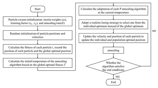
Figure 1.
Flowchart of the improved SA-PSO algorithm.
3. Case Study
To assess the efficacy of the optimization model and methodology in addressing injection–production optimization for extensive, depleted gas storage reservoirs, the W23 gas storage reservoir was selected as a case study. This reservoir is in the northern region of the Wenliu structural high, within the central uplift zone of the Dongpu sag. The overall geological structure is characterized by a complex anticline that has developed against a backdrop of basement uplift, which is segmented by regional level III and IV faults into four distinct blocks: the main block (W23), the east block, the west block, and the south block. According to the distribution of faults, the W23-UGS is further divided into seven blocks on the horizontal plane, namely W103, W109, W23-2, W105, W106, W22, and W23-5, as depicted in Figure 2a.
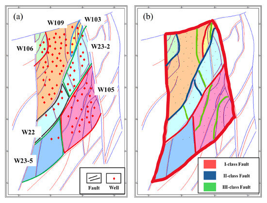
Figure 2.
Plane distribution map of W23-UGS: (a) layout and well location deployment, (b) fault distribution.
Based on the evaluation of fault sealing, the main faults of the W23-UGS are classified into three categories, namely I-Class faults to III-Class faults. I-Class faults have the strongest sealing ability and are regarded as strongly sealed faults. The connectivity between the blocks on both sides of these faults is extremely poor. During the injection and production processes, there is no mutual influence, and the formation pressure difference across the fault is greater than 10 MPa. II-Class faults come next, being weakly sealed faults. The connectivity between the two side blocks is relatively poor, with minor pressure interference, and the pressure difference across the fault is less than 10 MPa. III-Class faults have the poorest sealing ability and are non-sealed faults. The connectivity between the blocks on both sides is relatively good, and the formation pressure difference across the fault is less than 5 MPa. I-Class and II-Class faults are used as the criteria for dividing each block, and the fault classification is shown in Figure 2b.
The gas-bearing layer of W23 is located within the fourth member of the Shahejie Formation, which is part of the Lower Tertiary, at a burial depth ranging from 2750 to 3120 m. This member is further subdivided into eight distinct sand formations, exhibiting a total formation thickness of 300 to 500 m. The sand formations are characterized by significant thickness, stability, and favorable internal connectivity. The reservoir displays low porosity and low permeability, with porosity values ranging from 8.86% to 13.86% and permeability values between 0.27 and 17.12 millidarcies (mD). The methane content within the reservoir varies from 89.28% to 97.13%, while the condensate oil content is measured at 10 to 20 g per cubic meter (g/m3). The original formation pressure is recorded to range from 38.62 to 38.87 megapascals (MPa), and the original formation temperature is around 116 °C (PipeChina Zhongyuan gas storage co., ltd, Puyang City, Henan Province, China), indicating the presence of a sandstone gas reservoir with block-like characteristics. The caprock at the top of the Wen 23 gas reservoir mainly consists of grayish-white salt rocks and gypsum-salt beds deposited in the lower part of the third member of the Shahejie Formation, interbedded with gray and dark-gray mudstones. The gypsum-salt rocks in the Wen 23 area are characterized by a large thickness, wide distribution, and strong sealing ability.
The W23 gas storage reservoir was initially characterized by a formation pressure of 38.6 MPa and encompasses an area of approximately 8.15 km2. It is designed as a working gas volume with a total capacity of 10.365 × 10⁸ m3, which includes a working gas volume of 40.02 × 10⁸ m3. The project is structured into two distinct phases: Phase 1 is currently operational, while Phase 2 has been constructed but is not yet fully functional. Phase 1 is designed to accommodate a capacity of 84.31 × 10⁸ m3 and a working gas volume of 32.67 × 10⁸ m3, with operational pressures ranging from 20.92 to 38.6 MPa. The surface facilities are designed to support a maximum daily injection rate of 1800 × 104 m3/d and a maximum withdrawal rate of 3000 × 104 m3/d. Phase 2 contributes an additional capacity of 19.284 × 10⁸ m3 and a working gas volume of 7.35 × 10⁸ m3, with surface facilities capable of handling 600 × 104 m3/d for injection and 900 × 104 m3/d for withdrawal.
Phase 1 of the Wen-23 gas storage project comprises a total of 131 wells. This total includes 68 newly constructed wells, which consist of 58 injection-production wells, 3 gas-only production wells, 5 monitoring and observation wells, and 2 wells that are awaiting commissioning. Furthermore, there are 63 existing wells, which include 46 plugged wells, 6 monitoring wells located outside the block, and 11 repurposed wells situated within the block. In Phase 2, drilling has been completed for 24 wells, all of which are currently awaiting production. The locations of the wells for each block are illustrated in Figure 2a.
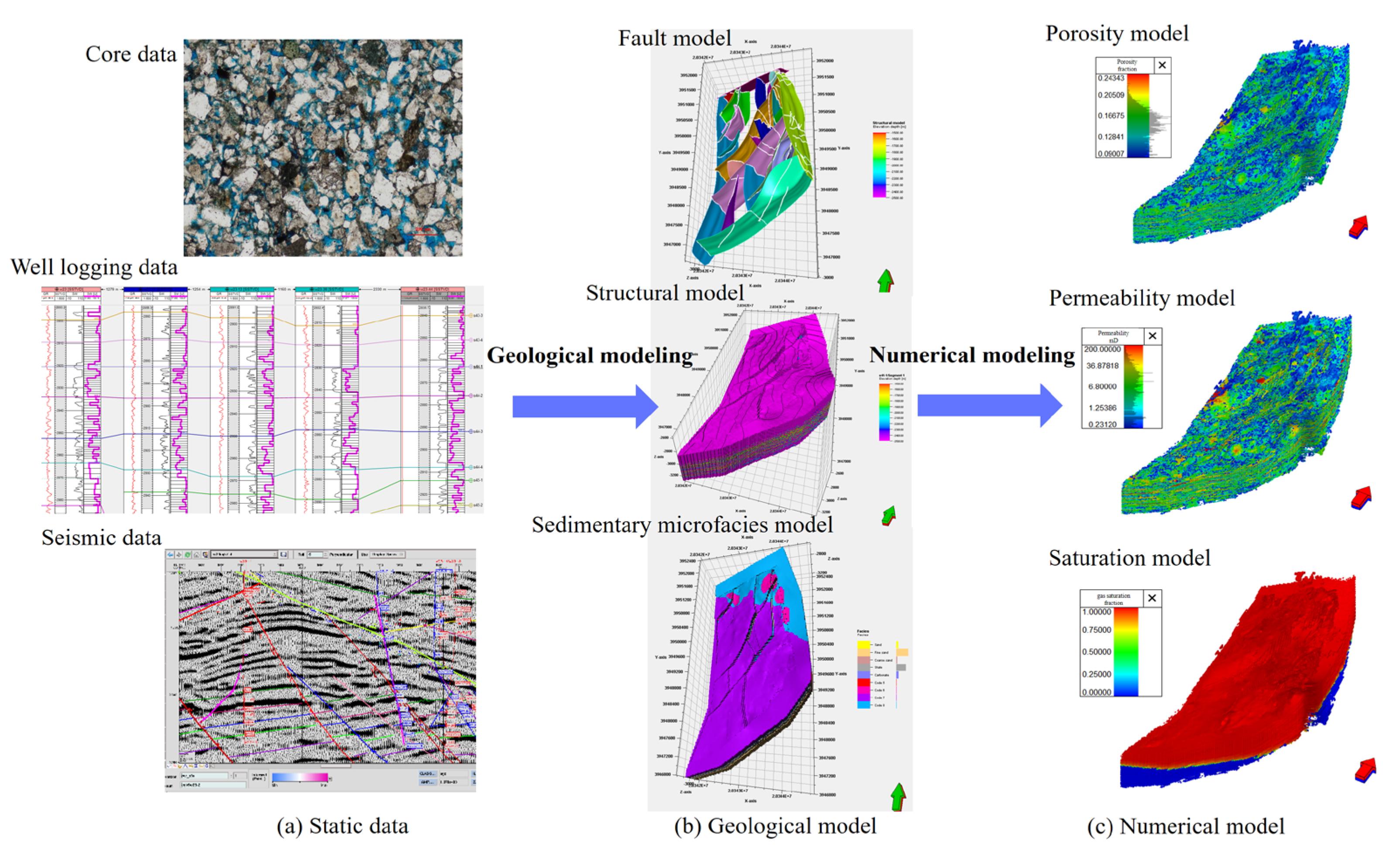
Before the implementation of injection–production optimization, it is essential to first establish a numerical simulation model to validate the subsequent optimization strategies. This study develops a three-dimensional geological model (Petrel 2016, Schlumberger Limited, Shenzhen, China) of the W23 gas storage reservoir, utilizing interpretations derived from core samples, well logs, seismic data, and other pertinent information. By employing this geological model and incorporating reservoir characteristics, flow mechanisms, and production data from 131 wells, a high-resolution numerical simulation model (tNavigator 22.4, Rock Flow Dynamics, Houston, TX, USA) of the W23 reservoir is constructed, as illustrated in Figure 3.

Figure 3.
W23-UGS modeling process: (a) static data, (b) geological model, (c) numerical model.
History matching constitutes a vital component in the process of reservoir numerical simulation. Upon completion of the numerical model computation, it is essential to compare the actual field injection and production data with the simulated results. The numerical model can only be deemed reliable and accurately reflective of the true reservoir dynamics when the simulation closely corresponds with the actual field data. Consequently, adjustments to parameters are necessary during the history-matching process to attain a high level of accuracy, which will subsequently inform analysis and forecasting endeavors.
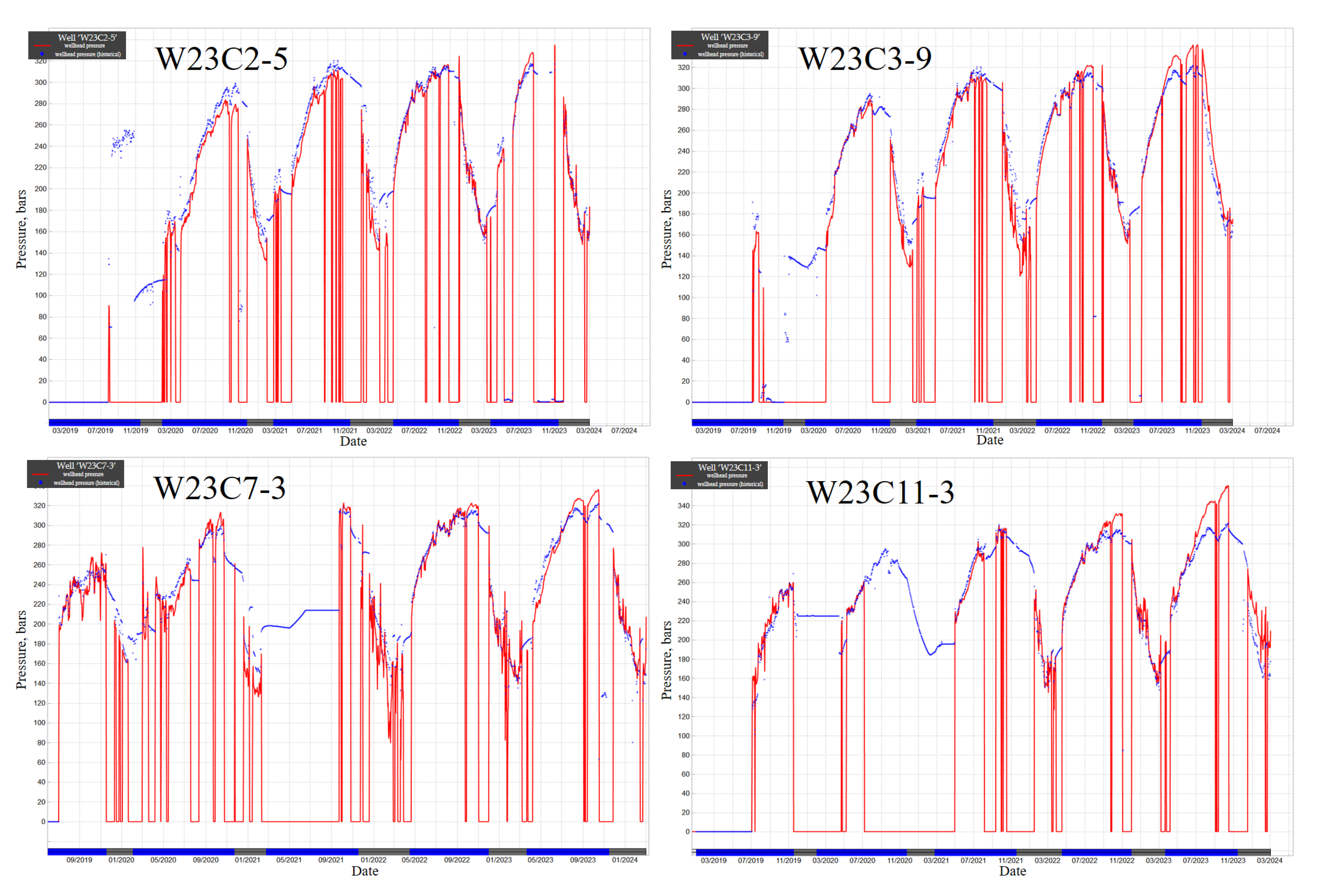
In the process of history matching, we conducted the matching by maintaining a constant surface gas production rate for the wells, utilizing key indicators such as bottom-hole pressure and wellhead pressure. This approach employs historical matching to assess the accuracy of the numerical model, with the pressure curves of representative injection and production wells serving as evaluation metrics. The results indicate that the model attained a high level of reservoir pressure matching (see Figure 4), thereby confirming the reliability of this numerical model in predicting pressure distribution within a highly complex geological environment. This validation establishes a solid foundation for the subsequent optimization of injection and production processes.
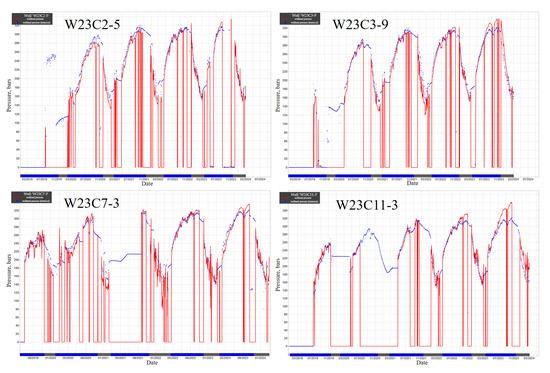
Figure 4.
Comparison of the predicted wellhead pressure from the numerical simulation model for the representative well with the actual pressure.
As of March 2024, the W23 gas storage reservoir has completed five injection–production cycles, resulting in a cumulative gas injection of 122.34 × 10⁸ m3 and a cumulative gas production of 64.89 × 10⁸ m3, leading to a net gas injection of 63.2 × 10⁸ m3. Following four years of operational activity, the reservoir has transitioned into a stable operational phase; however, the actual working gas volume has only reached 54.7% of its designed capacity. During the 2023–2024 cycle, the injection phase recorded a cumulative injection of 21.86 × 10⁸ m3, which constitutes 54.65% of the designed working gas volume. The peak daily injection rate during this period was 1787 × 104 m3/d, representing 74.46% of the maximum designed daily injection rate. Conversely, the production phase resulted in a cumulative gas output of 21.18 × 10⁸ m3, equivalent to 52.95% of the designed working volume, with a peak daily production rate of 3112 × 104 m3/d, amounting to 79.79% of the maximum designed daily injection rate.
In comparison to the design targets established for the reservoir, there exists potential for optimizing the working gas volume. The extensive faults in the W23 gas field have complicated the original injection–production plan. There are seven strongly sealed faults, three weakly sealed faults, and several non-sealed faults in the W23 gas field. The complex distribution of these faults poses challenges in maintaining the injection–production pressure balance across the entire fault block. Consequently, it is imperative to readjust the injection–production strategy during the stable production phase to enhance the working gas volume, equilibrate pressure differentials between the blocks, and ensure the efficient and stable operation of the gas storage reservoir.
Currently, the W23 gas storage reservoir is in the expansion phase, aiming to achieve its full production capacity. The inventory and storage capacity of each block at the conclusion of the fifth injection–production cycle are detailed in Table 1. For Phase 1, the feasibility report established the maximum injection and production capacities for 58 injection wells and 61 production wells under varying formation pressure conditions. Utilizing actual injection–production data from individual wells, the projected maximum injection capacity for the current 58 injection wells is presented in Table 2, while Table 3 illustrates the maximum production capacity for the 61 production wells under different geological conditions. It is important to note that the Phase 2 wells are not yet fully operational, and the maximum injection–production capacity per well is estimated based on geological parameters.

Table 1.
Inventory and storage capacity of each block before injection in the 6th cycle.
Table 2.
Designed maximum gas injection capacity under different formation pressure conditions.
Table 3.
Statistics table of gas production capacity for each well site in the UGS (unit: 104 m3/d).
The analysis of the gas injection capacity and varying formation pressures indicates that the actual gas injection capacity of the formation diminishes progressively during the later stages of gas injection, significantly falling below the levels observed during the initial injection phase. To speed up achieving optimal capacity, the strategy for the sixth cycle involves further increasing the formation pressure by injecting gas at the maximum injection capacity. It is anticipated that the maximum permissible gas injection volume for the Phase 1 project will reach 20.8 × 10⁸ m3, with an average formation pressure of 36.5 MPa after the injection period. For the Phase 2 project, the maximum permissible gas injection volume is projected to be 5 × 10⁸ m3, also with an average formation pressure of 36.5 MPa at the end of the injection. Based on the inventory and pressure variations observed throughout the five cycles, the current inventory equation for Phase 1 is as follows:
Based on the end-of-injection formation pressure of 36.5 MPa for this cycle, it is anticipated that gas production will reduce the formation pressure to 21.5 MPa, leading to an average decrease in information pressure of approximately 15 MPa. Utilizing the inventory equation, the cumulative gas production for Phase 1 is estimated to be 21.9 × 10⁸ m3, while the maximum permissible gas production volume for the Phase 2 project is projected to reach 5 × 10⁸ m3.
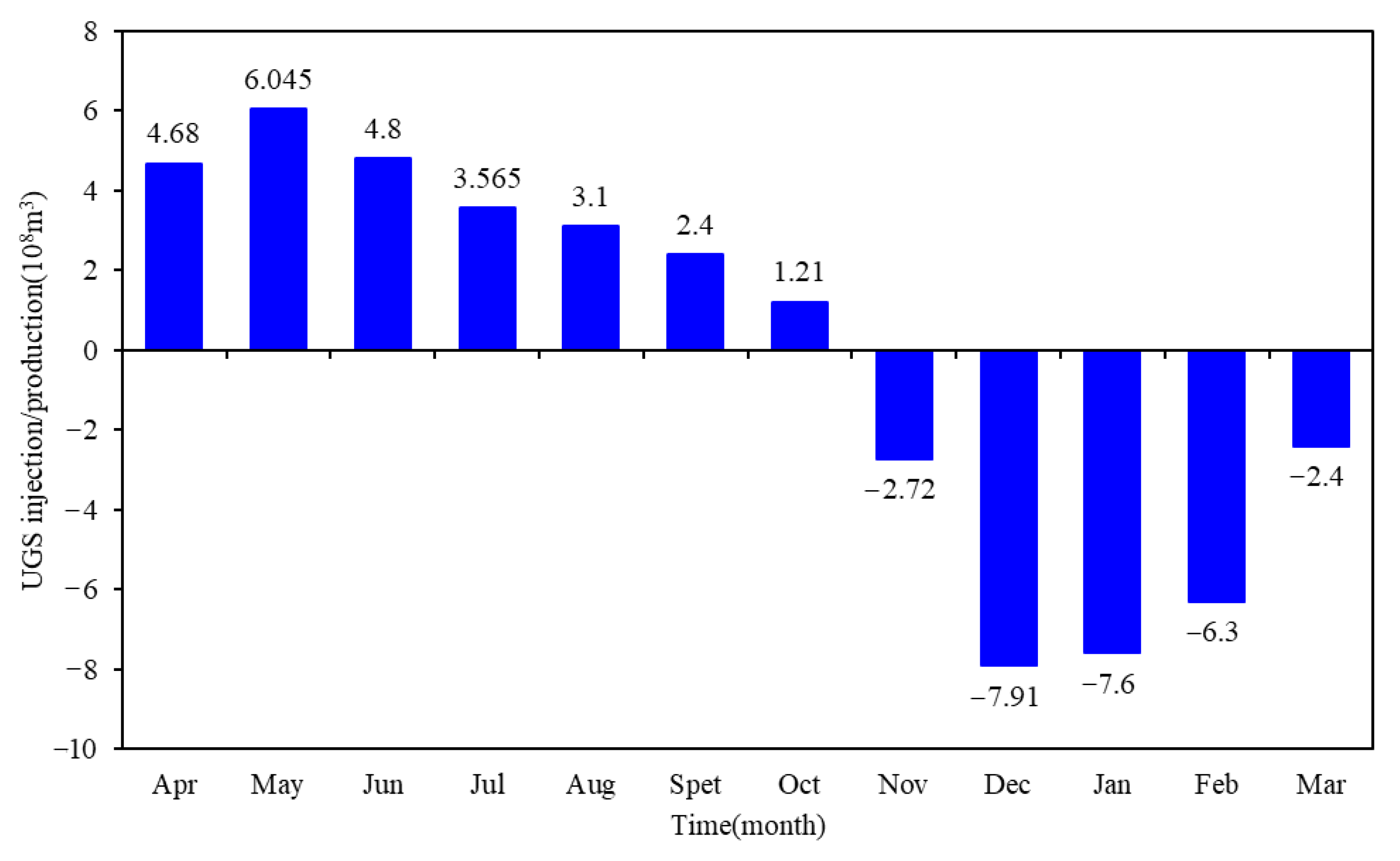
The monthly schedule for gas injection and production is depicted in Figure 5. An initial rapid injection phase occurs during the early to mid stages, which is subsequently followed by a gradual decline in the injection rate during the later stages. This approach facilitates a steady increase in formation pressure. It is anticipated that the gas injection rate will attain its peak between May and June, with over 70% of the total cumulative injection volume projected to be completed by the end of July. In September and October, the injection volume is expected to decrease gradually in response to the rising formation pressure, thereby mitigating the risk of excessive pressure accumulation around the wells. Furthermore, monthly adjustments to the injection schedule will be implemented based on prevailing market gas supply conditions.
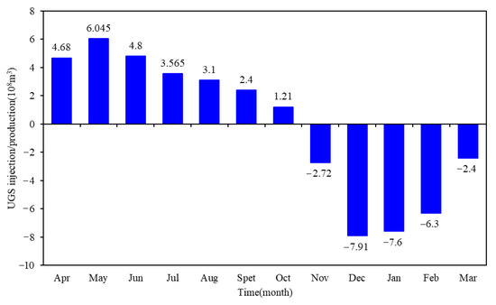
Figure 5.
Monthly gas injection and production plan for the 6th cycle of the W23-UGS.
4. Result
Based on the established relationship between block pressure and inventory, the SA-PSO algorithm is utilized to optimize the gas injection and production volumes for each block during the sixth injection–production cycle to minimize pressure differentials between blocks. This optimization process determines the most effective distribution of total gas injection and production volumes across the various blocks. Following this, and using the injection–production plan while considering the injection and production capacities of individual wells, the gas injection and production volumes for each well within each block are allocated. This completes the design of the injection–production scheme for the sixth cycle. The optimized gas injection and production volumes for each block are presented in Table 4.
Table 4.
Optimized allocation of gas injection and production volumes for each block in the 6th cycle.
To comprehensively illustrate the efficacy of the optimization model and the corresponding solution methodology, a comparative analysis is performed between the optimized injection–production scheme and the widely utilized empirical injection–production scheme within the field, following the acquisition of the optimized plan. The empirical scheme satisfies the total monthly gas injection and production requirements; however, it fails to consider the inter-block pressure differentials after injection. Instead, it allocates gas volumes exclusively based on the number of wells in each block and the capacity of individual wells.
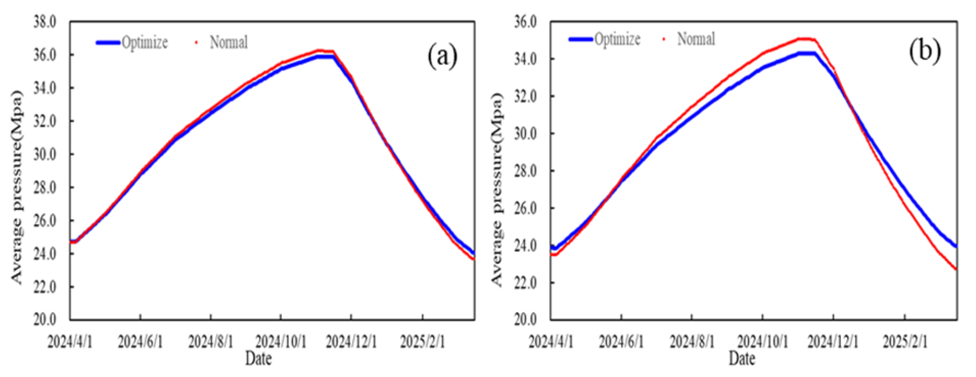
The optimized scheme was simulated utilizing modeling software, and the results were compared with those obtained from the empirical scheme. Figure 6 illustrates a comparison of the average formation pressure before and after optimization during the sixth injection–production cycle. The optimized scheme yields smaller variations in average formation pressure. In Phase 1 (Figure 6a), the optimized end-of-injection formation pressure (35.88 MPa) is marginally lower than the pre-optimization pressure (36.23 MPa), whereas the optimized end-of-production formation pressure (24.08 MPa) exceeds the pre-optimization pressure (23.68 MPa). Similarly, in Phase 2 (Figure 6b), the optimized end-of-injection formation pressure (34.31 MPa) is lower than the pre-optimization pressure (35.07 MPa), and the optimized end-of-production formation pressure (23.96 MPa) is greater than the pre-optimization pressure (22.75 MPa). These findings suggest that the optimized scheme has the potential to further enhance the working gas volume.
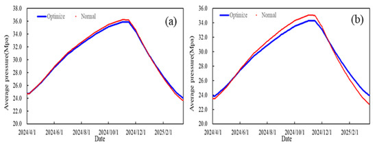
Figure 6.
Comparison of formation pressure before and after optimization in the 6th injection-production cycle of the W23-UGS: (a) Phase 1, (b) Phase 2.
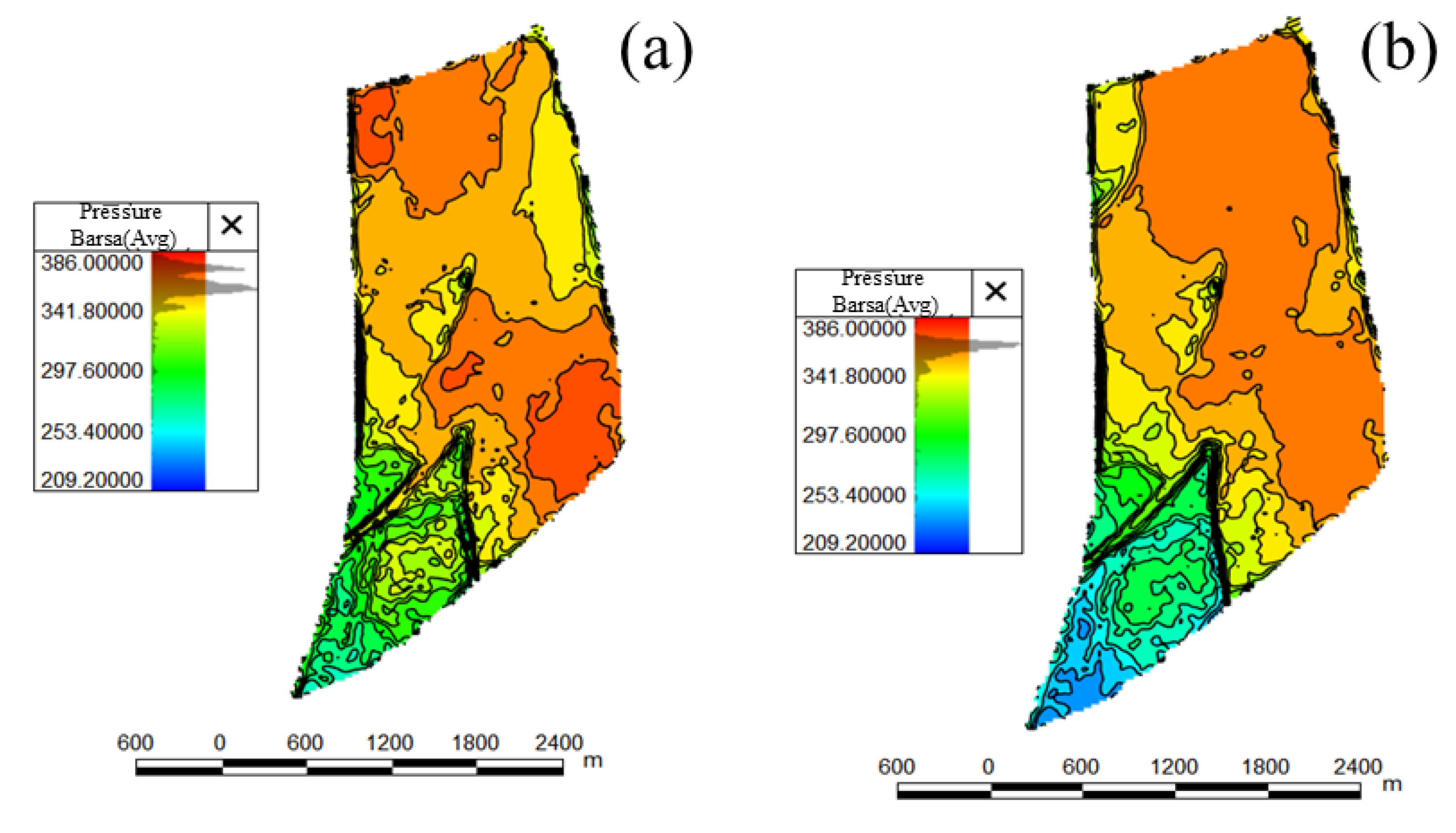
Utilizing the optimized scheme as input, the formation pressure distribution derived from this scheme was calculated and subsequently compared with the simulation results of the original scheme. The comparative analysis of the numerical models is illustrated in Figure 7 and Figure 8. As depicted in Figure 7, after the injection period, the optimized model demonstrates lower pressure readings in blocks W106, W23-5, and W22. With an equivalent total gas injection volume, the optimized scheme exhibits a more uniform pressure variation and reduced pressure differentials between the blocks. Figure 8 further indicates that at the end of the production period, the optimized model similarly reveals lower pressures in blocks W106, W23-5, and W22. Under the same total gas injection volume, the optimized scheme yields more gradual pressure changes and diminished inter-block pressure differences.
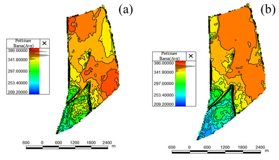
Figure 7.
Comparison of numerical model pressure distribution before and after optimization at the end of injection in the 6th injection–production cycle of the W23-UGS: (a) before optimization, (b) after optimization.
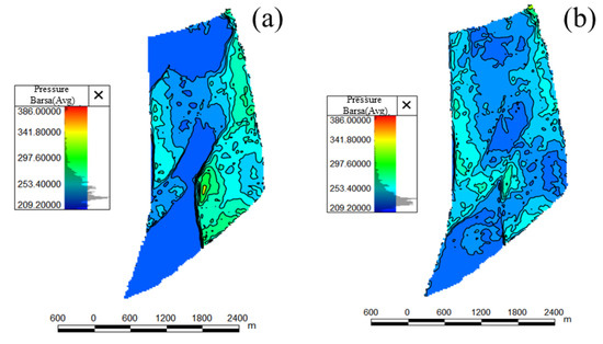
Figure 8.
Comparison of numerical model pressure distribution before and after optimization at the end of production in the 6th injection–production cycle of the W23-UGS: (a) before optimization, (b) after optimization.
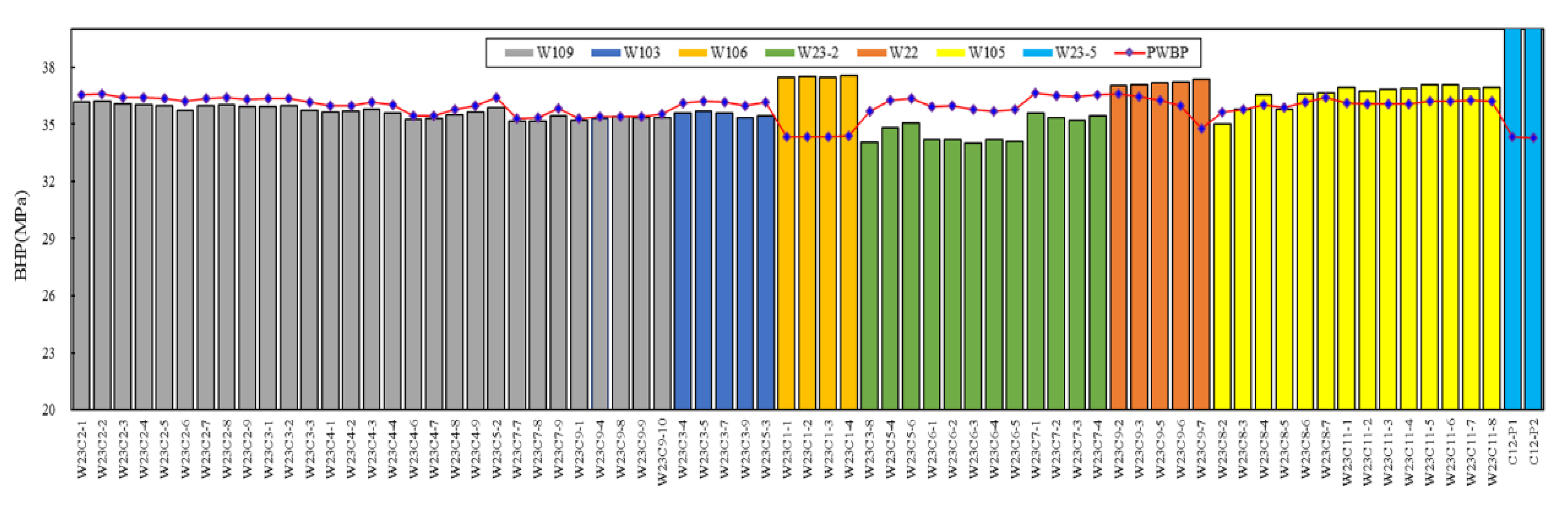
Figure 9 presents a comparative analysis of bottom-hole pressures for individual wells within each block after the injection phase during the sixth cycle, both before and after optimization. The red curve represents the pressure of the optimized model, while the bar chart illustrates the actual pressure recorded before optimization. Following the implementation of the optimized injection–production scheme, the distribution of bottom-hole pressures at the end of the injection phase demonstrates a more uniform profile in contrast to the pre-optimization condition. This modification effectively achieves the overall injection objectives without exceeding the formation pressure limits in any of the blocks.
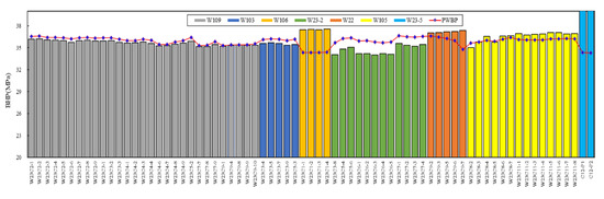
Figure 9.
Comparison of individual well bottomhole pressures in each block before and after optimization at the end of injection in the 6th cycle.
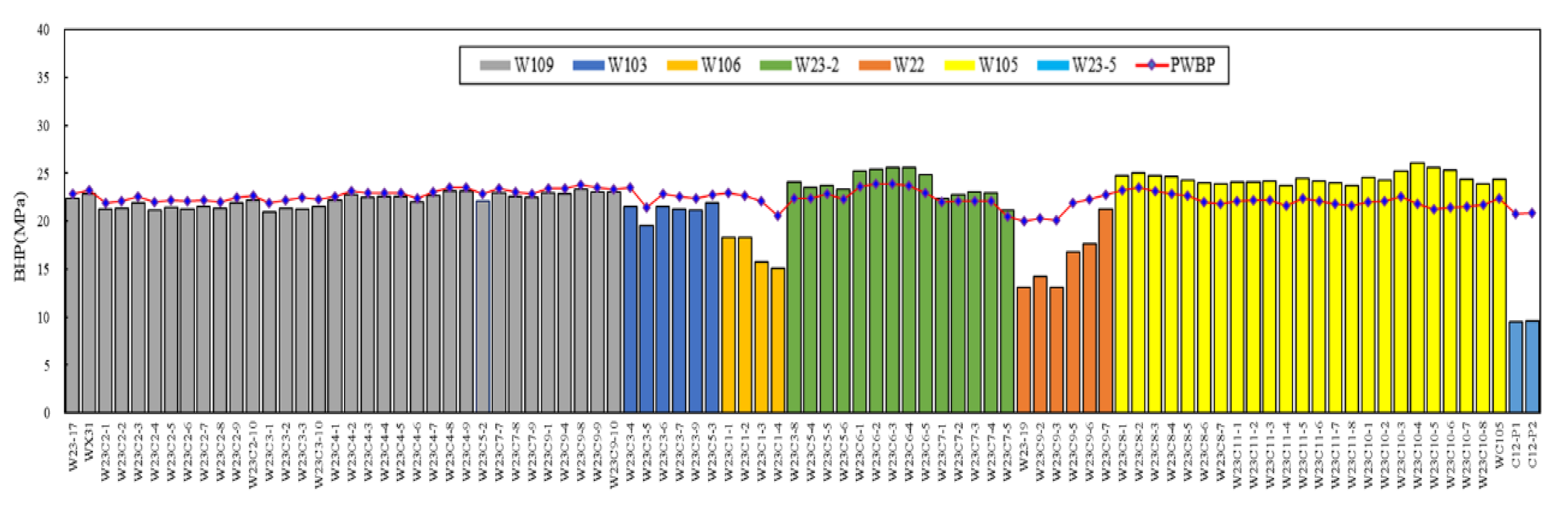
Figure 10 provides a comparative analysis of bottom-hole pressures across each block following production for the sixth cycle, both before and after the optimization process. The data demonstrate that the optimized scheme results in higher bottom-hole pressures after production when compared to the pre-optimization scenario. Additionally, due to the constraints imposed by the optimization model, regional pressures are sustained above the predetermined minimum threshold.
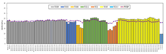
Figure 10.
Comparison of individual well bottomhole pressures in each block before and after optimization at the end of production in the 6th cycle.
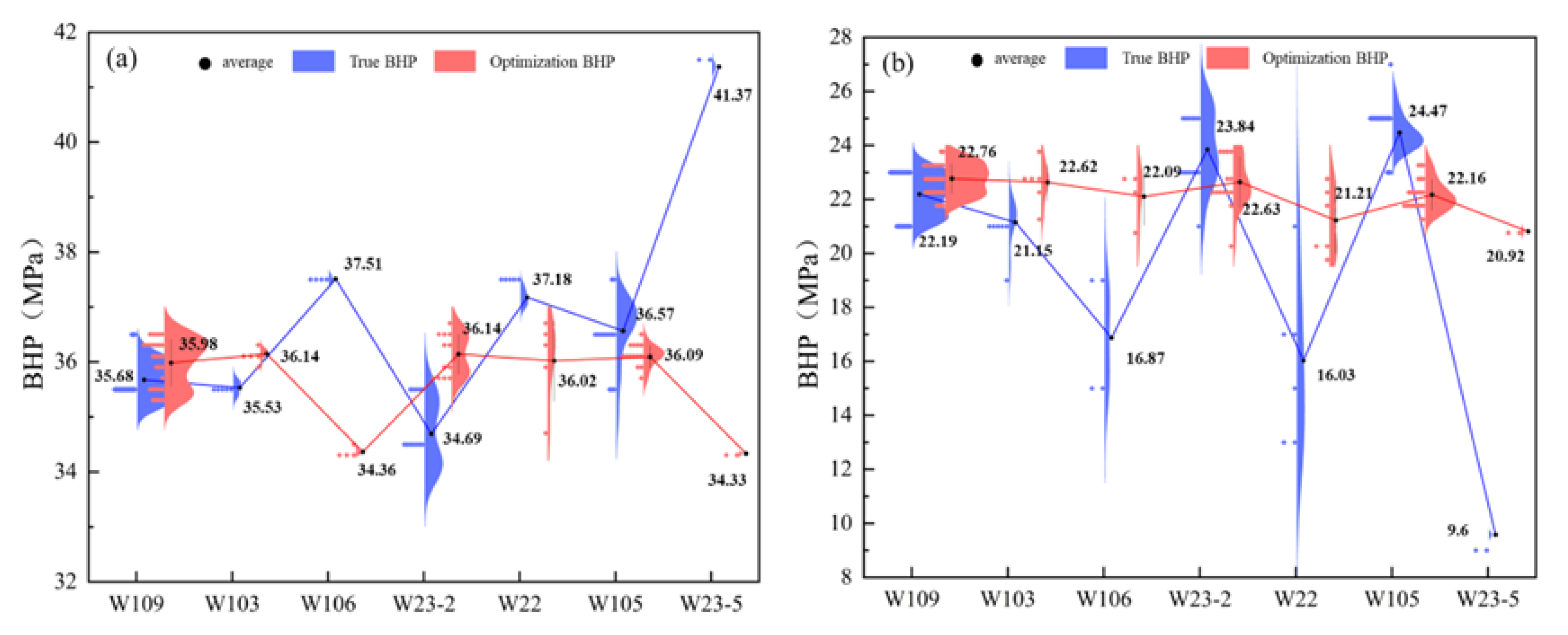
Figure 11 provides a comparative analysis of the average pressure in each block before and after the optimization process after the injection (Figure 11a) and production (Figure 11b) phases during the sixth injection–production cycle. The data are illustrated with blue representing pre-optimization pressures and red indicating post-optimization pressures. In Figure 11a, it is evident that before optimization, the pressure at the end of the injection phase for Well Block W106 was recorded at 37.51 MPa, W22 at 37.18 MPa, and W23-5 at 41.37 MPa, with several blocks exceeding the formation pressure threshold of 38.6 MPa. The variance in formation pressures across the blocks was calculated to be 4.985 MPa2. Following the implementation of the optimized injection–production strategy, the pressures at the end of the injection phase decreased to 34.36 MPa in W106, 36.02 MPa in W22, and 34.33 MPa in W23-5, resulting in a reduced variance of 0.618 MPa2, which represents one-eighth of the initial variance. In Figure 11b, the data indicate that prior to optimization, the pressures at the end of the production phase for Well Block W106 had declined to 16.87 MPa, W22 to 16.03 MPa, and W23-5 to 9.60 MPa, with certain blocks falling below the minimum formation pressure of 20.92 MPa. The variance of formation pressures across the blocks was determined to be 41.343 MPa2. Post-optimization, the end-of-production pressures increased to 22.09 MPa in W106, 21.21 MPa in W22, and 20.92 MPa in W23-5, thereby reducing the pressure variance across the blocks to 4.232 MPa2, which is one-tenth of the original variance.

Figure 11.
Comparison of average pressures in each block before and after optimization at the end of injection and production in the 6th cycle: (a) end of injection, (b) end of production.
5. Conclusions
- (1)
- To achieve a balanced variation in overall formation pressure during the production process of a gas storage facility, an optimization model for injection and production was developed to minimize the variance in formation pressures across different blocks following each operational cycle. Utilizing the W23 gas storage facility as a case study, a model grounded in the SA-PSO algorithm was formulated. This model demonstrated a significant reduction in pressure differentials between blocks during the sixth injection–production cycle. The reduction in the inter-block pressure difference can effectively prevent gas channeling or leakage accidents caused by the damage of fault sealing. The optimized allocation of injection and production volumes enhanced the operational efficiency of the gas reservoir, effectively addressing the limitations associated with traditional operational methodologies.
- (2)
- The establishment of a high-precision three-dimensional geological model, coupled with comprehensive numerical simulations, provided a robust foundation for the optimization process. By integrating real-time data and conducting historical matching, we ensured that the model accurately reflected the dynamics of the reservoir. The successful validation of these models affirms their efficacy in simulating the intricate geological conditions present at W23 and underscores their practical significance in informing future operational strategies.
- (3)
- A comparative analysis between the optimized injection–production strategy and conventional empirical methods revealed the tangible advantages of the new approach. The results indicate that the variance in formation pressures between blocks under the optimized framework is markedly lower than that observed with the empirical method, with the variance reduced to one-eighth of its original value. The optimized strategy not only augmented the working gas capacity but also preserved balanced pressures across blocks, effectively reducing the risks associated with excessively high pressures and salt precipitation. The precipitated salt crystals come from the gypsum-salt caprock above the gas field. Excessively low formation pressure causes the salt from the overlying layer to crystallize and precipitate into the formation and wellbore. As a result, the gas flow channels are blocked, the physical properties of the reservoir deteriorate, the power consumption of the compressor increases during the injection–production process, and the working gas volume decreases. This highlights the potential of SA-PSO-based optimization to enhance the efficiency and reliability of gas storage facilities, thereby ensuring the safe and stable operation of the gas storage reservoir.
Author Contributions
Conceptualization, X.B. and T.G.; methodology, X.B.; software, B.Y.; validation, X.B. and Y.L.; formal analysis, T.G.; investigation, J.Y.; resources, X.B. and F.H.; data curation, S.Z.; writing—original draft preparation, W.D.; writing—review and editing, Z.Z.; visualization, X.B. and W.D.; supervision, X.B.; project administration, X.B.; funding acquisition, T.G. All authors have read and agreed to the published version of the manuscript.
Funding
This research was funded by the PipeChina Energy Storage Technology Co., Ltd. (Grant number: KJ202303).
Data Availability Statement
The data presented in this study are available on request from the corresponding author.
Conflicts of Interest
Authors Xuefeng Bai, Tong Gu, Bo Yu, Yun Liu, Jiakun Yang, Famu Huang and Siyuan Zhang were employed by the PipeChina Energy Storage Technology Co., Ltd. The remaining authors declare that the research was conducted in the absence of any commercial or financial relationships that could be construed as a potential conflict of interest. The PipeChina Energy Storage Technology Co., Ltd., had no role in the design of the study; in the collection, analyses, or interpretation of data; in the writing of the manuscript, or in the decision to publish the results.
References
- Safari, A.; Das, N.; Langhelle, O.; Roy, J.; Assadi, M. Natural gas: A transition fuel for sustainable energy system transformation? Energy Sci. Eng. 2019, 7, 1075–1094. [Google Scholar] [CrossRef]
- Huang, K.; Zhang, W.; Wang, F.; Luan, Z.; Hu, Y.; Chen, J.; Fang, Y.; Song, Z.; Wang, J. Development status of underground space energy storage at home and abroad and geological survey suggestions. Geol. China 2024, 51, 105–117. [Google Scholar]
- Sedaee, B.; Mohammadi, M.; Esfahanizadeh, L.; Fathi, Y. Comprehensive modeling and developing a software for salt cavern underground gas storage. J. Energy Storage 2019, 25, 100876. [Google Scholar] [CrossRef]
- Animah, I.; Shafiee, M. Application of risk analysis in the liquefied natural gas (LNG) sector: An overview. J. Loss Prev. Process Ind. 2020, 63, 103980. [Google Scholar] [CrossRef]
- Chen, S.; Zhang, Q.; Wang, G.; Zhu, L.; Li, Y. Investment strategy for underground gas storage facilities based on real option model considering gas market reform in China. Energy Econ. 2018, 70, 132–142. [Google Scholar] [CrossRef]
- Jelušič, P.; Kravanja, S.; Žlender, B. Optimal cost and design of an underground gas storage by ANFIS. J. Nat. Gas Sci. Eng. 2019, 61, 142–157. [Google Scholar] [CrossRef]
- Firme, P.A.L.P.; Roehl, D.; Romanel, C. Salt caverns history and geomechanics towards future natural gas strategic storage in Brazil. J. Nat. Gas Sci. Eng. 2019, 72, 103006. [Google Scholar] [CrossRef]
- Malakooti, R.; Azin, R. The optimization of underground gas storage in a partially depleted gas reservoir. Pet. Sci. Technol. 2011, 29, 824–836. [Google Scholar] [CrossRef]
- Guo, W.; Zhang, B.; Liang, Y.; Qiu, R.; Wei, X.; Niu, P.; Zhang, H.; Li, Z. Improved method and practice for site selection of underground gas storage under complex geological conditions. J. Nat. Gas Sci. Eng. 2022, 108, 104813. [Google Scholar] [CrossRef]
- Khalili, Y.; Ahmadi, M. Reservoir modeling & simulation: Advancements, challenges, and future perspectives. J. Chem. Pet. Eng. 2023, 57, 343–364. [Google Scholar]
- Labadie, J.W. Optimal operation of multireservoir systems: State-of-the-art review. J. Water Resour. Plan. Manag. 2004, 130, 93–111. [Google Scholar] [CrossRef]
- Bagci, A.S.; Ozturk, B. Performance analysis of horizontal wells for underground gas storage in depleted gas fields. In SPE Eastern Regional Meeting; SPE: Houston, TX, USA, 2007; p. SPE-111102-MS. [Google Scholar]
- Tureyen, O.I.; Karaalioglu, H.; Satman, A. Effect of the wellbore conditions on the performance of underground gas-storage reservoirs. In SPE Unconventional Resources Conference/Gas Technology Symposium; SPE: Houston, TX, USA, 2000; p. SPE-59737-MS. [Google Scholar]
- Moradi, B. Study of gas injection effects on rock and fluid of a gas condensate reservoir during underground gas storage process. In SPE Latin America and Caribbean Petroleum Engineering Conference; SPE: Houston, TX, USA, 2009; p. SPE-121830-MS. [Google Scholar]
- Surej, S.; Burgstaller, C.; Fuller, J.; Wielemaker, E.; Jilg, W. Solving completion options for underground gas storage through geomechanics. In SPE Eastern Regional Meeting; SPE: Houston, TX, USA, 2008; p. SPE-116409-MS. [Google Scholar]
- Ponomareva, I.N.; Martyushev, D.A.; Govindarajan, S.K. A new approach to predict the formation pressure using multiple regression analysis: Case study from Sukharev oil field reservoir–Russia. J. King Saud Univ.-Eng. Sci. 2024, 36, 694–700. [Google Scholar] [CrossRef]
- Sircar, A.; Yadav, K.; Rayavarapu, K.; Bist, N.; Oza, H. Application of machine learning and artificial intelligence in oil and gas industry. Pet. Res. 2021, 6, 379–391. [Google Scholar] [CrossRef]
- Lambora, A.; Gupta, K.; Chopra, K. Genetic algorithm-A literature review. In Proceedings of the 2019 International Conference on Machine Learning, Big Data, Cloud and Parallel Computing (COMITCon), Faridabad, India, 14–16 February 2019; IEEE: Piscataway, NJ, USA, 2019; pp. 380–384. [Google Scholar]
- Wang, D.; Tan, D.; Liu, L. Particle swarm optimization algorithm: An overview. Soft Comput. 2018, 22, 387–408. [Google Scholar] [CrossRef]
- Karaboga, D. Artificial bee colony algorithm. Scholarpedia 2010, 5, 6915. [Google Scholar] [CrossRef]
- Price, K.V.; Storn, R.M.; Lampinen, J.A. The differential evolution algorithm. In Differential Evolution: A Practical Approach to Global Optimization; Springer: Berlin/Heidelberg, Germany, 2005; pp. 37–134. [Google Scholar]
- Bertsimas, D.; Tsitsiklis, J. Simulated annealing. Stat. Sci. 1993, 8, 10–15. [Google Scholar] [CrossRef]
- Wu, J.; Li, Z.; Sun, Y.; Cao, X. Neural network-based prediction of remaining oil distribution and optimization of injection-production parameters. Pet. Geol. Recovery Effic. 2020, 27, 85–93. [Google Scholar]
- Fadilah, S.M.R.; Aditsania, A. Optimization of gas injection allocation to increase oil production using Gbest-guided artificial bee colony algorithm. In Journal of Physics: Conference Series; IOP Publishing: Bristol, UK, 2019; Volume 1192, p. 012049. [Google Scholar]
- Farahi, M.M.M.; Ahmadi, M.; Dabir, B. Model-based multi-objective particle swarm production optimization for efficient injection/production planning to improve reservoir recovery. Can. J. Chem. Eng. 2022, 100, 503–520. [Google Scholar] [CrossRef]
- Azamipour, V.; Assareh, M.; Mittermeir, G.M. An improved optimization procedure for production and injection scheduling using a hybrid genetic algorithm. Chem. Eng. Res. Des. 2018, 131, 557–570. [Google Scholar] [CrossRef]
- Zhang, Y.; Wang, S.; Ji, G. A comprehensive survey on particle swarm optimization algorithm and its applications. Math. Probl. Eng. 2015, 2015, 931256. [Google Scholar] [CrossRef]
- Kennedy, J.; Eberhart, R. Particle swarm optimization. In Proceedings of the ICNN’95—International Conference on Neural Networks, Perth, WA, Australia, 27 November–1 December 1995; IEEE: Piscataway, NJ, USA, 1995; Volume 4, pp. 1942–1948. [Google Scholar]
- Zhang, Z.; Gan, H.; Zhang, C.; Jia, S.; Yu, X.; Zhang, K.; Zhong, X.; Zheng, X.; Shen, T.; Qu, L.; et al. Experimental Study on Improving Oil Recovery Mechanism of Injection–Production Coupling in Complex Fault-Block Reservoirs. Energies 2024, 17, 1505. [Google Scholar] [CrossRef]
- Ma, X.; Zheng, D.; Shen, R.; Wang, C.; Luo, J.; Sun, J. Key technologies and practice for gas field storage facility construction of complex geological conditions in China. Pet. Explor. Dev. 2018, 45, 507–520. [Google Scholar] [CrossRef]
- Syed, Z.; Lawryshyn, Y. Risk analysis of an underground gas storage facility using a physics-based system performance model and Monte Carlo simulation. Reliab. Eng. Syst. Saf. 2020, 199, 106792. [Google Scholar] [CrossRef]
- He, Z.; Tang, Y.; He, Y.; Qin, J.; Hu, S.; Yan, B.; Tang, L.; Sepehrnoori, K.; Rui, Z. Wellbore salt-deposition risk prediction of underground gas storage combining numerical modeling and machine learning methodology. Energy 2024, 305, 132247. [Google Scholar] [CrossRef]
- Zhang, J. Pore pressure prediction from well logs: Methods, modifications, and new approaches. Earth-Sci. Rev. 2011, 108, 50–63. [Google Scholar] [CrossRef]


Disclaimer/Publisher’s Note: The statements, opinions and data contained in all publications are solely those of the individual author(s) and contributor(s) and not of MDPI and/or the editor(s). MDPI and/or the editor(s) disclaim responsibility for any injury to people or property resulting from any ideas, methods, instructions or products referred to in the content. |
© 2025 by the authors. Licensee MDPI, Basel, Switzerland. This article is an open access article distributed under the terms and conditions of the Creative Commons Attribution (CC BY) license (https://creativecommons.org/licenses/by/4.0/).