Article

Power Load Forecasting System of Iron and Steel Enterprises Based on Deep Kernel–Multiple Kernel Joint Learning

1
Beijing Research Institute of Ansteel Co., Ltd., Beijing 102200, China
2
The State Key Laboratory of Rolling and Automation, Northeastern University, Shenyang 110819, China
*
Author to whom correspondence should be addressed.
Processes 2025, 13(2), 584; https://doi.org/10.3390/pr13020584
Submission received: 13 December 2024 / Revised: 11 February 2025 / Accepted: 12 February 2025 / Published: 19 February 2025

Abstract

:
The traditional power load forecasting learning method has problems such as overfitting and incomplete learning of time series information when dealing with complex nonlinear data, which affects the accuracy of short–medium term power load forecasting. A joint learning method, LSVM-MKL, was proposed based on the bidirectional promotion of deep kernel learning (DKL) and multiple kernel learning (MKL). The multi-kernel method was combined with the input layer, the highest coding layer, and the highest encoding layer to model the network of the stack autoencoder (SAE) to obtain more comprehensive information. At the same time, the deep kernel was integrated into the optimization training of Gaussian multi-kernel by means of the nonlinear product to form the nonlinear composite kernel. Through a large number of reference datasets and actual industrial data experiments, it was shown that compared with the Elman and LSTM-Seq2Seq methods, the proposed method achieved a higher prediction accuracy of 4.32%, which verified its adaptability to complex time-varying power load forecasting processes and greatly improved the accuracy of power load forecasting.

1. Introduction

Electricity is very important in the production processes of steel enterprises, accounting for about 90% of the total energy loss [1]. Power load forecasting is based on historical load data to predict the total electricity consumption in future periods. Accurate load forecasting can guide steel enterprises’ production planning, rational power purchase, and the reasonable arrangement of equipment maintenance and repair, and improve their economic efficiency. Because of the non-stationarity, non-linearity, complexity, and dynamic nature of load data, it is challenging to accurately forecast the short- and medium-term load. The traditional load forecasting methods are mainly based on statistical models, which cannot fully explore the inherent laws and dynamic changes in power loads [2]. In recent years, deep learning has achieved significant results in the field of temporal prediction, and kernel learning-based pattern analysis is able to efficiently handle nonlinear and temporal features in systems [3]. Multiple new data-driven methods have been proposed, and reference [4] proposed a deep learning-based LSTM (Long Short-Term Memory) Seq2Seq load forecasting model. The algorithm is prone to gradient vanishing and exploding as the number of layers and training iterations increases. A mid-term load forecasting model based on the Elman neural network was proposed [5], which used an improved BP algorithm to predict the load values of the regional power grid for the next 12 months of the year. However, the algorithm had problems with a slow rate of convergence and local minima [6].
In contrast, deep kernels based on deep neural networks have nonlinear mapping expressions. They only use the highest hidden layer of neural networks to construct kernels, requiring a large amount of data to ensure the information quality of the highest hidden layer, and there is an overfitting problem [7,8,9]. This paper proposes a bidirectional promotion joint learning method that improves the performance of deep kernels using multi-kernel learning, while using deep kernels to improve the training process of Gaussian multi-kernels [10]. A deep kernel prediction model with adaptive time-varying characteristics is established, and a special correlation layer is introduced into the multi-layer feedforward network to form a network with a “memory” ability [11], which can map the nonlinear and dynamic characteristics of the power load forecasting system. This combined model can exploit more abstract potential features from multiple angles of massive data, reflect the nonlinear and dynamic characteristics of the system, and overcome the problems of slow convergence and local minimal points [12]. The power load forecasting system of the steel enterprise adopts a mixed structure of B/S and C/S and implements deep learning algorithm functions in Python. The experimental results show that the method proposed not only effectively improves the accuracy of kernel learning, but also has a stronger universality to the dataset. It can meet the higher accuracy and adaptability requirements of production data, and can deal with the challenges of nonlinearity and the randomness of power energy forecasting, considering the incomplete learning of time-sequence information [13]. According to the entire process from theory to practical application, it can be divided into fundamental research methods and the deep multi-kernel joint learning model of experimental data.

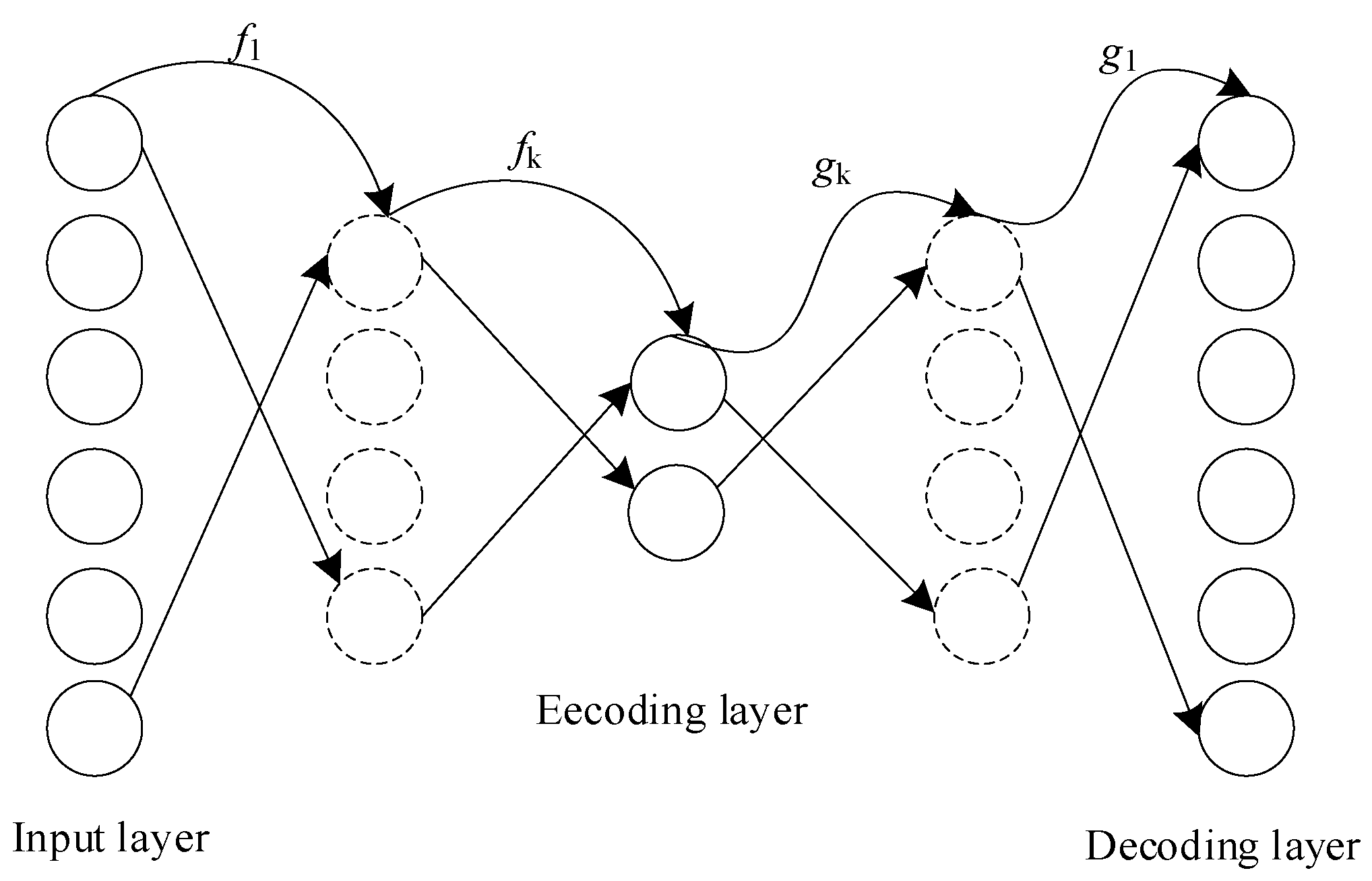
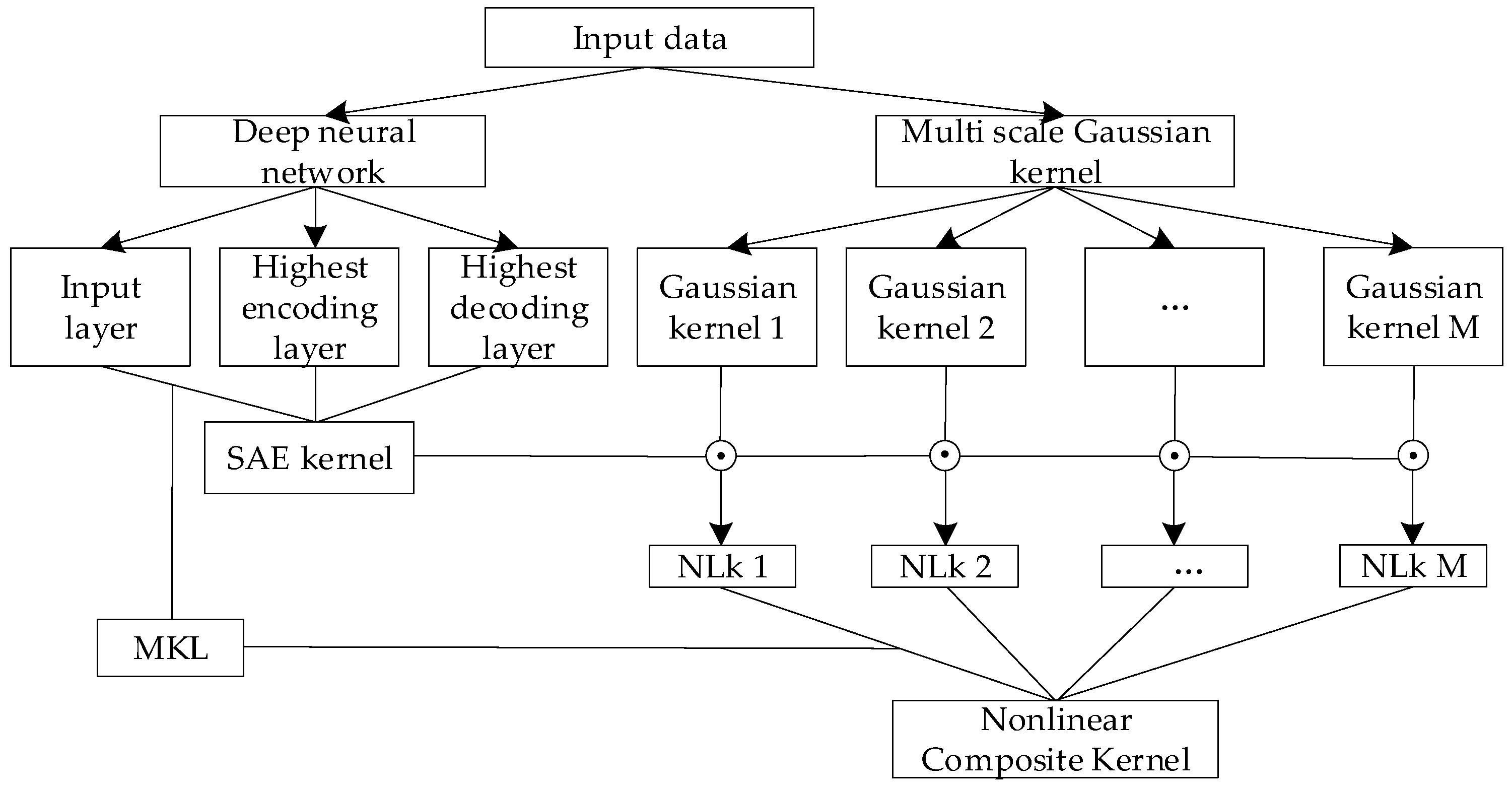
2. Deep Multi-Kernel Joint Learning Model

The kernel method is one of the methods that transforms nonlinear inseparable problems in low-dimensional spaces into linearly separable problems in high-dimensional spaces [14]. Multi-kernel learning is a linear or nonlinear combination of basic kernels, which takes the form of a convex combination of base kernels, that is, a linear non-negative combination of weight vectors with a fixed 1-norm:
k μ x i , x j = r = 1 M u r k r x i , x j = r = 1 M u r φ r x i , φ r x j u r 0 , u 1 = 1
where kμ is the combination of base kernels, φr is the feature map from the original space to the high-dimensional Hilbert space, kr is the r-th kernel (the Gaussian kernel or the polynomial kernel), ur is the r-th kernel weight vector, and M is the number of multiple kernels. The multi-kernel can capture different data similarity information, effectively combine them to adapt to different modalities of information, and reduce the workload of selecting kernel hyperparameters by directly learning the base kernel weights from the data.
The deep neural network relies on a stacked series of nonlinear mappings to learn representations through the increasing complexity of feature levels. The mathematical model can be described by a nonlinear function φnet from the input space to the output space. In typical feedforward neural networks, it is defined as a combination of basic mapping functions:
φ n e t x = ψ o u t ψ l ψ 2 ψ 1 x
where Ψ1 is the mapping from the input layer to the first layer, Ψout is the mapping from the highest layer to the output, and ◦ is the iteration between mappings. The nonlinear mapping from the hidden layer of r − 1th to the hidden layer of rth is
ψ r x = σ W r x + b
where Wr is the weight matrix, b is the bias, and σ is the activation function. The kernel function constructed based on the deep neural network approximation kernel mapping idea has an explicit function expression form. Kernel mapping transforms the original input space into a feature space using neural networks, and the deep kernel mapping function is expressed as:
K d = ψ n K n ψ 1 K 1 = σ W n K n σ W 1 K 1 + b 1 + b n
As shown in Figure 1, in response to the problems of incomplete information and overfitting in deep kernels, a multi-kernel method is adopted to combine the input layer, highest encoding layer, and highest decoding layer of the SAE kernel, which improves the expressive ability of the deep kernel. The obtained deep kernel is integrated into the optimization training of Gaussian multi-kernels in a nonlinear multiplication manner, and they are coordinated with each other to form a nonlinear combination kernel [15]. NLk1.. M means the deep information of nonlinear kernels.
As shown in Figure 2, the network representations of the input layer, the highest encoding layer, and the highest decoding layer of the SAE core are combined and reconstructed [16]. The number of layers in the deep autoencoder are set to 2k + 1, with the 0th layer as the input layer. The first to k th layers are set as the encoding layers. The k + 1th to 2kth layers are set as the decoding layers. The nonlinear mapping function between each layer of the encoding layer is fr (x), and the nonlinear mapping function between the decoding layers is gr (x),
ψ r ( x ) = x f 0 f 1 f r g r g 1 = ψ r 1 x f r g r , 0 r k
Among them, ψ 0 x = x as the input, and the internal representation of the hidden layer were determined through calculations performed by continuously applying the basic mapping ψ 0 , ψ 1 , ψ 2 . Among them, f1, … fk are the nonlinear mapping functions from the input layer to the encoding layer, and g1, …, gk are the nonlinear mapping functions from the encoding layer to the decoding layer.
Figure 2. Stack autoencoder structure.
Processes 13 00584 g002
Given that the encoder layer can automatically and effectively extract high-dimensional data and map it to low-dimensional hidden data:
k 0 x i , x j = x i , x j k 1 x i , x j = φ k x i , φ k x j k 2 x i , x j = ϕ k x i , ϕ k x j
Three kernels containing different depth information can be obtained, and the SAE core can be integrated through a multi-kernel method.
The organic combination of deep kernel learning and multi-kernel learning achieves the coordinated training and joint learning between the deep kernel and multi-kernel, improving the flexibility of the model. The algorithm process is as follows:
Step 1: Predefine the hyperparameters such as network layers, number of neurons, training algorithm, activation function, etc., and train the deep autoencoder using unsupervised pretraining and fine-tuning methods.
Step 2: Extract the highest encoding layer representation φ k x , the highest decoding layer representation ϕ k x , and the input layer representation ϕ 0 x from the network, and kernel the Equation (4).
Step 3: Integrate the three types of kernelling layers from Step 2 using a multi-kernel, and determine the hyperparameters using empirical and experimental methods.
Step 4: Predefine M Gaussian basis kernels g 1 , …, g M . Each kernel is multiplied with the deep autoencoder kernel obtained in Step 3 to obtain a set of nonlinear kernels k 1 , …, k M .
Step 5: Use the same multi-kernel method and kernel parameters as in Step 3 to optimize the k 1 , …, k M combinatorial optimization to form a nonlinear combinatorial kernel.
Step 6: Apply the obtained nonlinear combination and the kernel machine parameters (Lagrange multipliers and biases) from Step 5 for classification.

3. Experimental Results and Analysis

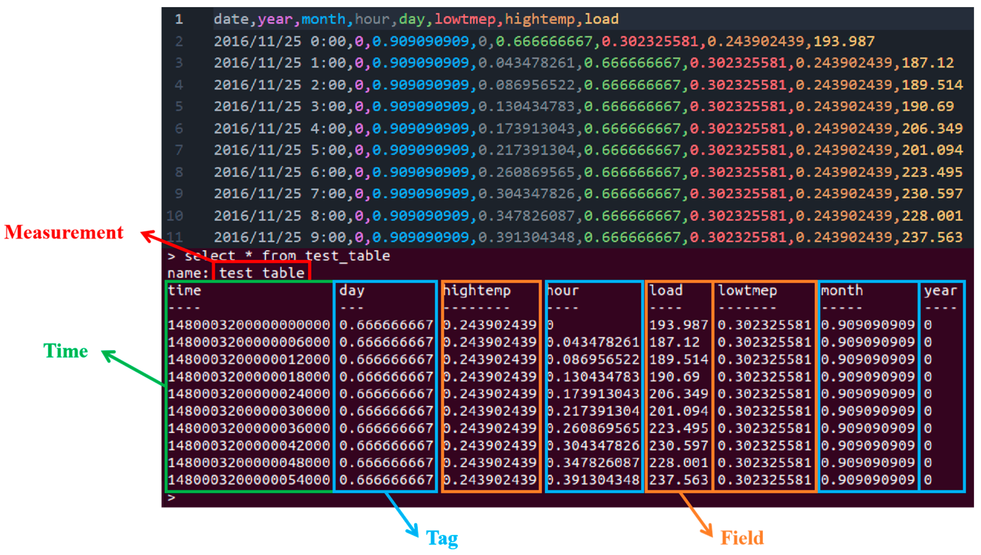
3.1. Benchmark Dataset

In order to ensure data timeliness, the data are divided into a sequence every ten days on a daily basis, and the total load value for the next ten days is predicted based on the process losses and power load consumption values of the ten days. Experiments are conducted on 15 benchmark datasets with different features and sample sizes. The data have been preprocessed and normalized, and the prediction accuracy is used to evaluate the performance of the model. The information of the dataset is compared before and after optimization, and the accuracy results are shown in Table 1. The prediction accuracy is the average of 20 random experiments, with 70% of the samples randomly selected as the training set and 30% as the testing set.
Three data-driven methods for instantiation are used, such as LSVM-MKL, Elman, and LSTM-Seq2Seq [17]. Based on this, comparative experiments are conducted using SAE (AE), Gaussian multi-kernel (Gau), and joint methods (G-A). The kernel learning machine and hyperparameter settings are the same. Elman uses a three hidden layer regression neural network and trains the network by an improved BP algorithm (an adaptive learning rate momentum gradient descent backpropagation algorithm) [18]. The encoder part of the LSTM-Seq2Seq model consists of 10 sets of LSTM modules stacked in a two-layer LSTM network [19]. The number of hidden layers is set to 24, and the initial states are all zero. The weight initialization is a normal distribution with a mean of 0 and a variance of 1. The LSVM-MKL penalty parameter is 1, and the maximum number of iterations is 10,000 using hard spaced SVM. The hyperparameter is 0. The multi-scale Gaussian kernel set has kernel widths of {5−2, 5−1, 50, 51, 52, 53, 54}, and the SAE kernel network has seven layers. Adam is used for training, and the activation function is ReLU For nonlinear functions, the kernel width and ReLU have a stronger expressive power, especially in deep networks. ReLU has a constant gradient in the non-negative interval, so there is no gradient vanishing problem, which maintains the convergence speed of the model in a stable state.
As shown in Figure 3, after the comprehensive comparison of the three methods, the joint method achieved excellent results, with the highest classification accuracy on datasets 13, 10, and 12. Compared with the Gaussian multi-kernel method, it improved almost all of the 15 datasets and had significant effects on some datasets. Under LSVM-MKL, the accuracy improvements of the HOR, OOC1, OOC2, SON, PRO, BAN, and SPL datasets were 2.94%, 2.57%, 3.15%, 3.66%, 5.19%, 4.37% and 2.58% respectively. Under Elman, the improvement levels of the MON1, MON2, SON, and PRO datasets were 2.94%, 2.57%, 3.15%, and 3.66%, respectively. Under LSTM-Seq2Seq, the improvement levels of the OOC1, OOC2, and PRO datasets were 2.09%, 2.26%, and 4.44%, respectively. Overall, in the high-dimensional datasets of HOR, OOC2, SON, PRO, and BAN, the SAE kernel has a strong feature extraction ability and integrates prior information into Gaussian multi-kernel training.
The good results in datasets with lower dimensions, such as MON1, MON2, MON3, and BLO, further demonstrate that our method has good universality and stability, and can be applied to multiple types of data. On the other hand, the joint approach is not simply about neutralizing the kernel under two systems, but rather integrating the advantages of both. In the ION, SON, and MON1 datasets, the method can still achieve high-precision prediction, indicating that it can eliminate the influence of adverse factors and prefers to select the best one to achieve the optimal combination state of the two kernel systems.

3.2. Power Load Forecasting

This prediction system is developed in the Micro Visual Studio 2010 environment. Net technology is used to design the web interface, and the C # language is used to complete the layout of the system pages. SQL Server 2019 is selected as the database to complete data access functions. The Python 3.1 uses TensorFlow, and the neural network structure adopts an unsupervised model autoencoder network. As shown in Figure 4, it is a partial screenshot of the dataset. The historical load data and environmental collection information (such as temperature, humidity, air pressure, etc.) obtained from the power system will be processed for missing/NaN values, seasonal adjustments, noise removal, outlier handling, and stability checks to obtain the preprocessed load data.
To address this issue, a power load forecasting model is established, and the prediction target is set as the active power of electricity. The input data includes historical day parameters, holiday definitions, scheduling maintenance plans, loading load data (source data), and modifying source data. Load forecasting includes setting forecast dates, conducting medium- to short-term load forecasting, compiling forecast results, and adjusting forecast results. Data output includes adding curves, deleting curves, clearing the screen, refreshing, comparing curves, displaying all of the algorithm results, and conducting assessment statistics. As shown in Figure 5a, the dataset comes from the active power consumption of 800–1400 MW in a certain steel enterprise in the first 11 months of 2023, and the active power in the 12th month is predicted, with a total of 2880 records. Considering the real-time requirements of the actual production process, the efficient LSVM-MKL was selected for the experiment, with a multi-scale Gaussian set kernel width of {5−1, 50, 51, 52, 53, 54}.
As shown in Figure 5b, compared with the actual value, the predicted load for December 2023 is basically in the middle of the actual value, with an average relative error of 4.32%. Using the LSVM-MKL model for prediction, the neural networks can better fit the relationship between the input and output. With the increase in information sources, this method achieves the highest prediction accuracy. Therefore, this method has been proven to be adaptable and effective for complex time-varying industrial problems, and can meet the working conditions of different processes. Overall, the average relative error of the electricity load forecasting system for steel enterprises in 2024 is within 5% to avoid the penalty price settlement of electricity bills. The maximum demand is accurately predicted based on the dynamic load, and the peak demand is reduced by the load dispatch measures, which directly reduces the expenditure for purchased electricity.

4. Conclusions

Aimed at the problems of poor stability and unsatisfactory prediction accuracy caused by the nonlinear and temporal characteristics of power load forecasting, a joint learning model based on the multi-kernel is proposed for steel enterprises. The effectiveness of the model is ultimately verified through experiments. It constructs a more flexible kernel learning framework by the joint bidirectional learning between the data-driven SAE kernel and Gaussian multi-kernel, which improves the expression ability of the kernel.
In the experiment, the prediction accuracies of three prediction models were compared, and prediction accuracy showed a different performance on different data types. The LSVM-MKL model had a higher prediction accuracy, training iteration speed, and stability. Comparison with the Elman and LSTM-Seq2Seq, the feasibility and effectiveness of the joint learning methodit was further demonstrated.
Due to the poor learning ability of the Elman and LSTM-Seq2Seq models for power load temporal information, the joint models outperformed the other two models in terms of training iteration speed and stability, and the average relative error was improved to 4.32%. In the model, only historical load data was considered as input, without taking into account the influence of other factors. In future studies, temperature and weather conditions can be included to further improve the prediction accuracy.

Author Contributions

Conceptualization, Y.Z., J.W., J.S., R.S. and D.Q.; methodology, Y.Z.; software, Y.Z. and J.W.; validation, Y.Z., J.W., J.S. and D.Q.; formal analysis, Y.Z. and R.S.; investigation, D.Q.; resources, J.S.; data curation, Y.Z., J.W. and R.S.; writing—original draft preparation, Y.Z. and J.W.; writing—review and editing, Y.Z. and J.S.; visualization, Y.Z. and D.Q.; supervision, Y.Z.; project administration, Y.Z. and J.W. All authors have read and agreed to the published version of the manuscript.

Funding

This research was funded by the National Key Research and Development Program Funding Project (Grant No. 2022YFB3304800).

Data Availability Statement

The data that support the findings of this study are available from the corresponding author, Yan Zhang, upon reasonable request.

Conflicts of Interest

Authors Yan Zhang, Junsheng Wang, Ruiqi Sun and Dawei Qin were employed by Beijing Research Institute of Ansteel Co., Ltd. The remaining authors declare that the research was conducted in the absence of any commercial or financial relationships that could be construed as a potential conflict of interest.

References

  1. Luo, X.; Chen, F.; Lu, Y.; Zhao, Z.; Peng, Y.; Pang, J. Intelligent Fault Diagnosis Method for Transformer Driven by Multiple Vibration Data. J. Phys. Conf. Ser. 2024, 2774, 4255–4262. [Google Scholar] [CrossRef]
  2. Li, H.; Li, Y.; Huang, J.; Shen, C.; Wang, C.; Jing, T.; Liu, Z.; Xu, W. Physical Metallurgy Guided Industrial Big Data Analysis System with Data Classification and Property Prediction. Steel Res. Int. 2022, 93, 3029–3043. [Google Scholar] [CrossRef]
  3. Gonen, M.; Alpaydin, E. Multiple kernel learning algorithms. J. Mach. Res. 2011, 12, 2211–2268. [Google Scholar]
  4. Anan, M.; Kanaan, K.; Benhaddou, D.; Nasser, N.; Qolomany, B.; Talei, H.; Sawalmeh, A. Occupant-Aware Energy Consumption Prediction in Smart Buildings Using a LSTM Model and Time Series Data. Energies 2024, 17, 6451. [Google Scholar] [CrossRef]
  5. He, Z.; Li, C.; Shen, Y.; He, A. A Hybrid Model Equipped with the Minimum Cycle Decomposition Concept for Short-Term Forecasting of Electrical Load Time Series. Neural Process. Lett. 2017, 46, 1059–1081. [Google Scholar] [CrossRef]
  6. Arvanitidis, A.I.; Bargiotas, D.; Daskalopulu, A.; Laitsos, V.M.; Tsoukalas, L.H. Enhanced Short-term Load Forecasting using Artificial Neural Networks. Energies 2021, 14, 7788. [Google Scholar] [CrossRef]
  7. Li, Y.; Zhang, T.; Hu, H. Deep Kernel Mapping Support Vector Machine based on Multilayer Perceptron. J. Beijing Univ. Technol. 2016, 42, 1652–1661. [Google Scholar]
  8. Wang, Q.; Lv, Z.; Wang, L.; Wang, W. Long Term Prediction Model based on Deep Denoising Kernel Mapping. Control Decis. 2019, 34, 989–996. [Google Scholar]
  9. Ma, L.; Dong, J.; Peng, K. A Novel Hierarchical Detection and Isolation Framework for Quality-related Multiple Faults in Large-scale Processes. IEEE Trans. Ind. Electron. 2020, 67, 1316–1327. [Google Scholar] [CrossRef]
  10. Jiao, J.F.; Yu, H.; Wang, G. A Quality-related Fault Detection Approach Based on Dynamic Least Squares for Process Monitoring. IEEE Trans. Ind. Inform. 2016, 63, 2625–2632. [Google Scholar] [CrossRef]
  11. Han, M.; Zhang, H. Multiple Kernel Learning for Label Relation and Class Imbalance in Multi-label Learning. Inf. Sci. 2022, 613, 344–356. [Google Scholar] [CrossRef]
  12. Geng, Z.; Li, S.; Yu, F. Ulta-short-term and Short-term Power Load Single-step and Multi-step Prediction Considering Spatial Association. Comput. Eng. 2024, 7, 22–25. [Google Scholar]
  13. Aiolli, F.; Donini, M. Easymkl. A Scalable Multiple Kernel Learning Algorithm. Neurocomputing 2015, 169, 215–224. [Google Scholar] [CrossRef]
  14. Wang, G. Research on Theory and Algorithm of Support Vector Machine. Ph.D. Thesis, Beijing University of Posts and Telecommunications, Beijing, China, 2008; pp. 1–30. [Google Scholar]
  15. Hassanzadeh, S.; Danyali, H.; Karami, A.; Helfroush, M.S. A Novel Graph-Based Multiple Kernel Learning Framework for Hyperspectral Image Classification. Int. J. Remote Sens. 2024, 45, 3075–3103. [Google Scholar] [CrossRef]
  16. Wang, T.; Zhang, L.; Hu, W. Bridging Deep and Multiple Kernel Learning: A Review. Inf. Fusion 2021, 23, 18. [Google Scholar] [CrossRef]
  17. Uğurel, E.; Huang, S.; Chen, C. Learning to Generate Synthetic Human Mobility Data: A Physics-Regularized Gaussian Process Approach based on Multiple Kernel Learning. Transp. Res. Part B 2024, 189, 103064. [Google Scholar] [CrossRef]
  18. Mori, H.; Kurata, E. An Efficient Kernel Machine Technique for short-term Load Forecasting under Smart Grid Environment. In Proceedings of the 2012 IEEE Power and Energy Society General Meeting, San Diego, CA, USA, 22–26 July 2012. [Google Scholar]
  19. Hernandez, L.; Baladron, C.; Aguiar, J.M.; Carro, B.; Sanchez-Esguevillas, A.; Lloret, J. Artifical Neural Networks for Short-term Load Forecasting in Microgrids Environment. Energy 2014, 75, 252–264. [Google Scholar] [CrossRef]
Figure 1. Joint learning framework.
Processes 13 00584 g001
Figure 3. Classification accuracy under three kinds of multi-kernel instances. (a) LSVM-MKL1; (b) Elman1; (c) LSTM-Seq2Seq1; (d) LSVM-MKL2; (e) Elman2; and (f) LSTM-Seq2Seq2.
Processes 13 00584 g003
Figure 4. Datasets and timing databases.
Processes 13 00584 g004
Figure 5. Power load forecasting results. (a) Training values and actual values; and (b) predicted values and real values.
Processes 13 00584 g005
Table 1. Dataset information.
SerialDatasetSample SizeDimensionLSVM-MKL/
Before Optimization
ElmanNeural Network/
Before Optimization
Seq2Seqmodel/
BeforeOptimization
1MON1124 + 432687.73 ± 0.01/66.46 ± 0.0086.04 ± 0.17/67.25 ± 0.6287.18 ± 0.28/66.65 ± 0.01
2MON2169 + 432686.66 ± 0.28/65.60 ± 0.0186.60 ± 0.24/73.38 ± 0.0184.19 ± 0.36/65.19 ± 1.10
3MON3122 + 432695.37 ± 0.01/82.28 ± 0.1095.14 ± 0.01/82.12 ± 0.9095.08 ± 0.11/81.94 ± 0.00
4HOR300 + 682583.82 ± 0.01/80.81 ± 1.0983.75 ± 0.73/80.88 ± 0.0087.13 ± 0.64/81.32 ± 1.05
5OOC110224079.24 ± 2.62/76.67 ± 1.2680.19 ± 1.47/78.58 ± 1.2077.14 ± 1.35/75.05 ± 1.79
6OOC29122581.24 ± 1.28/79.84 ± 1.5178.86 ± 2.02/77.16 ± 1.7682.49 ± 1.41/80.23 ± 1.84
7ION3513495.06 ± 1.35/87.64 ± 1.3194.23 ± 1.17/87.70 ± 2.2994.97 ± 1.60/88.01 ± 2.06
8SON2086083.08 ± 4.01/76.88 ± 3.0284.38 ± 3.84/75.29 ± 1.9383.41 ± 3.44/77.21 ± 3.75
9SPL15356092.17 ± 1.91/90.05 ± 1.9692.02 ± 0.95/89.86 ± 1.4591.35 ± 1.65/90.23 ± 1.43
10BRE1699996.79 ± 0.81/86.43 ± 0.8196.63 ± 2.66/85.06 ± 1.0696.91 ± 0.78/86.73 ± 0.66
11BRE25693095.63 ± 2.01/84.86 ± 3.0293.72 ± 2.61/83.72 ± 2.6695.37 ± 2.35/85.21 ± 3.41
12PRO1065576.23 ± 7.49/74.53 ± 4.8377.08 ± 4.75/58.87 ± 2.6676.89 ± 6.48/75.57 ± 5.04
13CLI5401891.96 ± 1.27/81.96 ± 1.2892.28 ± 1.22/82.28 ± 1.2292.15 ± 1.46/82.15 ± 1.05
14BLO748578.03 ± 2.42/75.91 ± 1.3474.10 ± 2.94/72.35 ± 3.0278.58 ± 1.88/77.47 ± 1.28
15BAN5123571.13 ± 2.27/69.94 ± 2.7368.28 ± 4.42/66.15 ± 3.4772.79 ± 1.79/70.88 ± 2.10
Disclaimer/Publisher’s Note: The statements, opinions and data contained in all publications are solely those of the individual author(s) and contributor(s) and not of MDPI and/or the editor(s). MDPI and/or the editor(s) disclaim responsibility for any injury to people or property resulting from any ideas, methods, instructions or products referred to in the content.

