A Study of the Mixing Process Under Vertical Vibration with Different Initial Structures

Abstract

Resonance Acoustic Mixing (RAM) is an efficient mixing technique and holds significant application value in many fields, especially in the mixing of high-viscosity materials. Due to the one-time loading feature, different material structures formed during the feeding process may cause undesired irregularities in the mixing process, which is not conducive to maintaining the mixing consistency between different batches. However, in the analysis of multi-component mixtures, previous studies have often overlooked the impact of the initial material structure. This study delved into the mixing mechanism of RAM in viscous solid–liquid mixtures. By constructing a numerical model based on the Mixture model, simulations of gas–solid–liquid multiphase flows under different initial structures were conducted, and the reliability of the model was verified through experiments. The research results indicate that the mixing processes with different initial structures share similar temporal characteristics of being intense at first and then moderating, but their development trends vary. The mixing time of the structure with the solid on the upper part is shortened by about 10% compared with that of the structure with the solid on the lower part. The double-interface structure exhibits a significantly higher mixing efficiency than the single-interface structure, with the mixing time reduced by up to 41%. This study offers a theoretical basis for optimizing the parameters of resonant acoustic mixing and holds significant reference value for the refined operation of resonant acoustic mixing in the future.

1. Introduction

Mixing refers to the process of dispersing and blending two or more materials using mechanical or fluid dynamic methods to ultimately form a homogeneous mixture [1]. As an important chemical engineering technique, mixing serves as an essential basic unit operation in many industries. Traditional dispersion mixing technologies primarily employ methods such as kneading, stirring and ultrasonic treatment. These methods utilize the large shear forces, pressure or local cavitation in the mixing area to achieve dispersion of high-viscosity materials [2]. However, these methods can cause significant stress stimulation to the materials or even damage them during the operation, and they may also be accompanied by a sharp rise in local temperature, which is unacceptable in processes involving materials that are sensitive to force and heat [3]. Resonant Acoustic Mixing (RAM) is a process that may be used to mix a wide array of materials such as liquids (especially high-viscous liquids), non-Newtonian rheological materials and particles without the use of blades [4,5]. Standard RAM equipment can achieve the mixing of contents by inducing the container to undergo vertical harmonic motion [6]. The technique is especially suitable for processes that involve high-viscosity materials, where traditional paddle-based methods struggle to perform effectively [7,8]. RAM avoids the use of blades, so the mixture constituents come into contact only with themselves and the container walls [9]. This characteristic has already gained significant attention in the field of energy materials preparation [10], as it offers advantages such as reduced contamination and improved mixing efficiency without the need for mechanical agitation [11,12]. Additionally, RAM also possesses the characteristics of high material yield, ease of cleaning and flexibility [13]. In the preparation of viscous materials with RAM, it is usual to deploy the particulate dispersed phase with the continuous phase composed of liquid components in one time loading. The vibration excitation leads to mutual kneading and collision between materials, resulting in the uniform dispersion of the slurry and particles [14]. The mixing of slurry in this case is a gas–liquid–solid multiphase flow process, characterized by various accompanying phenomena and a complex dynamic [15]. The efficiency of particle dispersion in the liquid phase under different initial distributions can serve as a useful tool for analyzing the mixing process (

Table 1. Summary of the literature on viscous material mixing with the RAM system.

Authors	Research Theme	Key Finding
Khan et al. [16]	Numerical modeling of the mixing process of HMX and TNT with an RAM system	Vibration amplitude and frequency both influence the mixing efficiency of the RAM process.
Zhan et al. [17]	The mixing process of two liquids with different viscosities with an RAM system.	Liquid jets on the surface can facilitate the mixing process of the two liquids.
Huo et al. [18]	Free surface instability when mixing with an RAM system.	The deformation of the free surface in the RAM flow field is closely related to Faraday instability.
Wang et al. [19]	Numerical study of multiphase flow in an RAM system with POD method.	Mixing parameters affect the generation and development of vortices in the RAM flow field.
Ours	The effects of loading parameters on mixing time of high-viscosity liquids with an RAM system.	Mixing time of viscous materials is significantly affected by vertical loading structures in an RAM system

).

Past research on RAM has primarily focused on the experimental processes of preparing various mixtures using this technology [20,21,22,23,24,25,26], with many studies conducted in this field, while only a limited number of studies have been conducted on the numerical simulation of the RAM process. The Air Force Research Laboratory of United States first completed a numerical simulation based on the LESLEI3D platform. They simulated the mixing process of high-viscosity resin materials under the influence of resonant acoustic mixing, providing a digital perspective for in-depth understanding of this complex phenomenon. In the processing of the simulation results, the Fourier analysis method was innovatively applied, enabling researchers to clearly observe the key feature of vortex length scale. By accurately defining the minimum vortex size generated within the interval, the potential value of RAM technology in the mixing application of high-viscosity resins and nanomaterials was effectively evaluated, laying a solid foundation for subsequent related studies [27]. Qu et al. and Imdad et al. conducted research on the mixing of HMX and TNT, employing the Mixture model to perform two-dimensional and three-dimensional simulation, respectively. They analyzed the impact of factors such as mixing time, vibration amplitude and shape of container on the density gradient of the product and concluded that the highest mixing efficiency is achieved in a spherical container, and the better efficiency always comes with higher amplitude and frequency [16,28]. Zhan et al. analyzed the relationship between key parameters and dynamic characteristics based on a VOF model combined with the mechanical model of the RAM system. In the work on fluid–solid coupling in resonant acoustic mixing, they built a coupling model of a multi-degree-of-freedom system and two-phase fluids. They found fluid movement under vertical acoustic vibration changed its equivalent mass, altering the system’s natural frequency, making the excitation frequency deviate from resonance, and reducing the dynamic response. Increasing excitation amplitude could boost the response but worsen amplitude fluctuation; raising the frequency properly could make the system run at a new resonance frequency, reducing fluid movement’s impact. They proposed an excitation force adjustment strategy based on their findings [29]. Furthermore, they also analyzed the correlation between flow field morphology and parameters of low-solid content, providing a critical oscillation curve indicating adequate mixing of glycerin solutions [17,30]. Wang et al. established a CLSVOF model for gas–liquid–solid three-phase flows to investigate the dispersion characteristics of RAM flow fields. By employing a modal decomposition method, the flow fields under various oscillation accelerations and filling levels were decomposed to extract the energy distribution patterns and energy structures at different scales [19]. Huo et al. utilized phase field models and spectral analysis methods to investigate the mixing mechanism of power-law non-Newtonian fluids during the RAM process. It was discovered that Faraday instability led to the development of vortices from large scales to small scales, with frequency components distributed near the operating frequency, relying on nonlinear effects to excite single frequency components for mixing [31]. Shah et al. [32] studied the interaction between liquid surface waves and liquids under the action of sound waves. Previous studies have fully investigated the vibration mechanism at the very first period and the influence of factors such as amplitude and frequency, but have not fully considered the impact of the initial material structure on the mixing process.

In actual manufacturing processes, the performance of energetic materials is often enhanced by the addition of fine particulate additives [33].When using the RAM technology for in situ mixing of missile and engine charges, formulation materials composed of multiple components usually participate in the mixing. These materials are arranged in layers in the vertical direction within the container, forming a staggered initial structure. In the early promotion of the RAM technology, not requiring a specific loading sequence was regarded as one of the characteristics of this technology. This is feasible in other scenarios where the mixing sequence of different component materials is not critical.

However, during the in situ mixing and curing process of energetic materials, there is often a need for the uniform dispersion of minor-component materials such as high-energy particles and curing agents in the container. A random loading process can have an adverse impact on this requirement. For example, when the curing agent is mixed at different positions in the container in different sequences, the hardness of the energetic materials at different heights in the final container will vary, which directly affects the product performance. At different interfacial structures, the diffusion rate of these fine particles within the container cannot be determined, which can easily lead to a decrease in the consistency of product quality, thereby affecting the performance of these trace elements. Due to confidentiality reasons, the original data cannot be presented here. Different initial structures refer to the different relative sequences formed by the materials in the vertical direction within the container after the initial loading process.

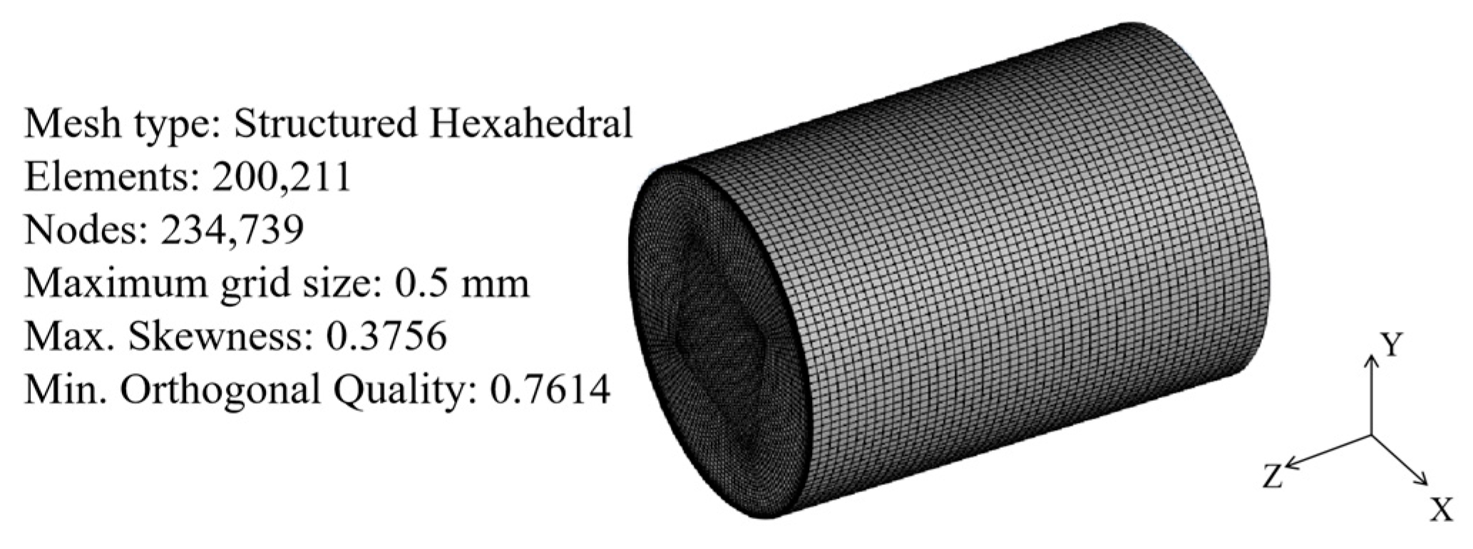
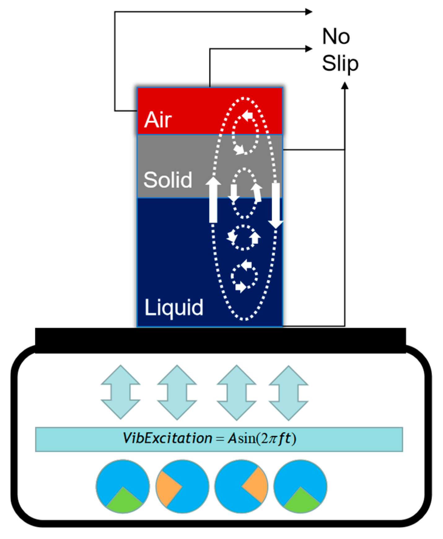
The key indicator that influences the performance of these trace elements is their uniform dispersion. Because of that, studying this characteristic at different initial material structures is of paramount importance for optimizing the parameters and for gaining a deeper understanding of the RAM process. This kind of research is currently lacking and further research is needed from the perspective of initial material structure to continue studying the mixing mechanism of the RAM process in high-viscosity mixtures. This study constructed a flow model based on the Mixture model and DPM model, focusing on the gas–liquid–solid multiphase flow of air, solid particle and viscous liquid. A set of numerical simulations were calculated with the initial material structure as variables. Based on the results, the uniformity of mixing and the distribution of particles over time of the flow field were compared to obtain the impact and relationship of variables on mixing efficiency. Comparisons are to be made with experimental data on the thoroughness of mixing to verify the findings. This study can provide a deeper insight into the RAM mechanism and a theoretical and data foundation for improving mixing efficiency.

2. Materials and Methods

2.1. Experimental Methods

The experimental platform utilizes a 100-milliliter resonant acoustic mixing system developed by Xi’an Modern Chemistry Research Institute (MCRI). During the experimental process, glycerin solutions (Chron Chemicals, Chengdu, China) and melamine powder (Huaxu Chemicals, Shijiazhuang, China) are employed as the liquid and solid phases, respectively. To simulate the actual production process, the filling rate is set to 90%. The properties used in the simulation are shown in

Table 2. Physical properties.

Material Property	Value
Particle Density	1.65 kg/m3
Particle diameter	0.1 mm
Liquid Density	1.26 kg/m3
Liquid Viscosity	1.41 Pa·s1

. High-speed photography experiments are conducted to document the relative flow states of particles and liquids. The motion of the container during the mixing process can be regarded as simple harmonic motion in the vertical direction, as described below:

$$z=Asin\left(2\pi ft\right).$$

(1)

In equation, A represents the amplitude, f represents the frequency and t represents the flow time.

2.2. Mixture Model

The formulation of composite energetic materials we discuss here has a solid content exceeding 10%. Among the commonly used multiphase flow models for solid–liquid mixtures, the Mixture model is suitable as the base model. The Mixture model allows the phases to be interpenetrating. The volume fractions for a control volume can therefore be equal to any value between 0 and 1, depending on the space occupied by different phases. The Navier–Stokes equation constitutes a system of conservation laws for mass, momentum and energy. In Cartesian coordinates, the conservation of mass equation may be written as follows [34]:

$${\displaystyle \frac{\mathsf{\partial }{\rho }_m}{\mathsf{\partial }t}}+\nabla ·\left({\rho }_m{\overrightarrow{v}}_m\right)=0,$$

(2)

where $v_m$ represents mass mean velocity, ${\rho }_m$ represents the mixture density:

$${\overrightarrow{v}}_m={\displaystyle \frac{\sum _{k=1}^n{\alpha }_k{\rho }_k{\overrightarrow{v}}_k}{{\rho }_m}},$$

(3)

$${\rho }_m={\sum }_{k=1}^n{\alpha }_k{\rho }_k,$$

(4)

where ${\rho }_m$ represents the density of the kth phase, ${\alpha }_k$ represents the volume fraction of the kth phase, ${\overrightarrow{v}}_k$ represents the velocity of the kth phase. The momentum equation for a mixture can be obtained by summing the individual momentum equations for all phases [35]:

$$\begin{gathered} {\displaystyle \frac{{\mathsf{\partial }\rho }_m{\overrightarrow{v}}_m}{\mathsf{\partial }t}}+\nabla ·{\rho }_m{\overrightarrow{v}}_m{\overrightarrow{v}}_m=-\nabla ·\mathrm{P}+\nabla ·\left[{\mu }_m\left(\nabla {\overrightarrow{v}}_m+{{\overrightarrow{v}}_m}^T\right)\right]+ \\ {\rho }_m\overrightarrow{g}+\overrightarrow{F}+\nabla ·\left({\sum }_{k=1}^n{\alpha }_k{\rho }_k{\overrightarrow{v}}_{dr,k}{\overrightarrow{v}}_{dr,k}\right), \end{gathered}$$

(5)

where n represents the phase index, $\overrightarrow{F}$ represents the body force, ${\mu }_m$ represents the viscosity of the mixture:

$${\mu }_m={\sum }_{k=1}^n{\alpha }_k{\mu }_k,$$

(6)

where ${\overrightarrow{v}}_{dr,k}$ represents the drift velocity of the kth phase. The Mixture model communicates the resistance forces between liquid phase and solid phase via ${\overrightarrow{v}}_{dr,k}$:

$${\overrightarrow{v}}_{dr,k}={\overrightarrow{v}}_k-{\overrightarrow{v}}_m.$$

(7)

2.3. Discrete Particle Model

To analyze the influence of different initial positions of fine particulate additives on the mixing effectiveness, the Discrete Phase Model was deployed to track the trajectory of inert particles released from the top, bottom and interfaces of the material. In a Lagrange coordinate system, the particle positions were calculated by integrating the force balance on each article without mutual interaction [36]. The balance between the particle inertia and external forces acting on the particles in x direction is defined as [37]

$${\displaystyle \frac{d{u}_p}{dt}}=F_D\left(u-u_p\right)+{\displaystyle \frac{g_x({\rho }_p-\rho )}{{\rho }_p}}+F_x,$$

(8)

where $u_p$ represents the particle velocity, $g_x$ represents the component of the gravitational acceleration in the x direction, $\rho$ represents the fluid density, ${\rho }_p$ represents the particle density, $F_x$ is a term including pressure gradient force, virtual mass force and Saffman’s lift force. $F_D\left(u-u_p\right)$ is the drag force per unit particle mass. $F_D$ is defined as

$$F_D=\left({\displaystyle \frac{18\mu }{{\rho }_p{d_p}^2}}\right)·\left({\displaystyle \frac{C_{D}Re}{24}}\right),$$

(9)

where $\mu$ represents the molecular fill level of the fluid, $d_p$ represents the particle diameter, Re represents the Reynolds number defined as

$$Re={\displaystyle \frac{{\rho }_p{d}_p\left|u_p-u\right|}{\mu }},$$

(10)

For spherical particles, the drag coefficient $C_D$ is defined as

$$C_D=a_1+{\displaystyle \frac{a_2}{Re}}+{\displaystyle \frac{a_3}{{Re}^2}},$$

(11)

where $a_1$, ${ a}_2$ and $a_3$ are given by Moris [38].

2.4. Boundary Conditions and Numerical Simulation Setup

The geometry for the RAM gas–liquid–solid flow simulation system is a typical cylinder as shown in Figure 1. The standard cylinder container has a diameter of 45 mm and is 80 mm in height. The remaining cylindrical surfaces are treated as “no-slip” walls. The oscillation applied for this work is described as follows with a fixed amplitude and angular frequency:

$$a={\displaystyle \frac{d^{2}z}{{dt}^2}}=-4{\pi }^2{f}^{2}Asin(2\mathsf{\pi }\mathrm{ft}),$$

(12)

The fluent UDF macro DEFINE_ADJUST provides an interface that could change the domain’s acceleration every time step. After interpretation, the function should be hooked in the User-Defined Function Hooks panel.

The RAM mechanism is shown in Figure 2. The RAM process utilizes the coupling that can occur between acoustic pressure or velocity fluctuations and fluctuating vorticity to facilitate the mixing process of materials. Adjacent layers of viscous fluid and solid particles are wrapped together by fluid loops of circulation established by the rotary motion existing in vortices. Viscosity is an important contributor to this process since it makes the fluid layers adhere to one another. The Reynolds number is dependent on the density of the fluid, the diameter of the particle and the viscosity of the fluid. The mixing process is closely related to the Reynolds number due to its impact on turbulence flow. However, the mixing problem we addressed here has a Reynolds number that is low enough to maintain a unity flow field. It follows that the Laminar model could be used for the situation. The pressure–velocity coupling is the pressure-implicit with the splitting of operator (PISO) method. The pressure discretization method is the pressure staggering option. The momentum discretization method is a second-order upwind scheme. The time step size is 0.0001 s. The numerical simulation was executed via Ansys Fluent in parallel version on a Think Workstation with 40 processors. Through a specific design, the particular manner in which components are introduced can synergize with the mixing mechanism of RAM, thereby enhancing the consistency of quality between batches. To achieve a more refined and consistent outcome in the homogenization process, we have engineered four initial relative orders of materials, which are sequentially introduced into the mixer before the commencement of mixing. At flow-time zero, the solid particles and liquid were patched to the specific initial regions. The initial regions are shown in Figure 3.

The geometry was meshed with Fluent Meshing. All zones were meshed with structured hexahedral grids. The element size was decided with a mesh independence test on different mesh numbers. Figure 4 shows the results of the vertical velocity distribution along the z-axis on the yz plane. The element quantities of the meshes were 90,445, 155,620, 200,211 and 296,087, respectively. To balance computational precision and efficiency, the configuration of mesh 3 was selected to apply for later simulation. To achieve better accuracy in calculating the fluid mixture, the adaptive mesh refinement technique was applied to refine the grid, with the density gradient on the grid serving as the refinement indicator.

In the context of this article, when dealing with the mixing of substances of the same mass, the mixing efficiency is defined as follows [39]: if we denote the mixing efficiency as E, the fixed mass of the substances as m and the mixing time as t, the relationship can be expressed as E = m/t. Specifically, given a fixed mass of substances to be mixed, the shorter the time it takes to achieve a homogeneous mixture, the higher the mixing efficiency. Here, a shorter t for the same m results in a higher E, indicating a more efficient mixing process. This definition reflects a shorter mixing time for an equal mass of materials, which not only means a faster rate of achieving a homogeneous state at the molecular or particulate level but also has significant implications for production efficiency and cost-effectiveness. The criterion for homogeneity in the mixture is that the difference between the maximum and minimum density values at all locations is less than 0.5 kg/m³ [16]. The mixing efficiency following the release of minor components from different initial positions is also a matter of concern. The amplitude and frequency of oscillation is fixed at 40 g and 60 Hz.

3. Results and Discussion

The gas–liquid–solid RAM process presents a complex flow environment. The reciprocating motion in the vertical direction causes materials at different heights to undergo disordered positional exchanges at staggered times, until a state of uniform mixing is achieved [40]. This study is to investigate the relationship between the initial structure and mixing performance.

High-speed photography is widely used to verify the authenticity of the interface deformation effect of the numerical model. In the research on the characteristics of the resonant acoustic flow field by Zhan et al. [41], the pictures of the liquid peak under different vibration frequencies and the pictures of the solid–liquid–gas mixing process with glycerin-sand obtained through high-speed photography proved the accuracy of the simulation results. In order to verify the numerical model proposed in this paper, in this section, the influence of different initial structures on the resonant acoustic mixing process is analyzed by comparing the output performance of the simulation model and the high-speed photographs over time. The experimental equipment consists of a high-speed photography system PFV4 (Photron FASTCAM Viewer 4) and a resonant acoustic mixing system developed by MCRI, as shown in Figure 5. To acquire the interphase mass-transfer characteristics, the numerical solution has been post-processed and the gross flow field structure has been examined at different snapshots in time. To illustrate the evolution of the mixing process, slices of the density field are shown. The slices are placed through the origin and are taken normal to the z planes.

3.1. Flow Analysis of Liquid–Solid Structure

Firstly, we discuss a category of situations where there is only a single interface between materials (not considering the interface with air). When it comes to mixing a liquid material with a solid material, two natural sequences emerge: the liquid–solid structure and the solid–liquid structure. To analyze the gas–liquid–solid mixing process under the liquid–solid structure, the distributions of tracer particles from different interfaces over time were extracted from the simulation model. High-speed photography was used to capture the motion of the fluid inside at a speed of 2000 frames per second for a comparison.

Figure 6 shows the comparisons between the distributions of tracer particles and the high-speed photographs at the corresponding times. Figure 6a shows the positions where particles released when at rest. When vertical vibration is initiated, the vibration energy spreads throughout the entire system. Particles at different heights will be directly or indirectly affected by the vibration energy. This vibration energy can overcome some initial adhesive forces, frictional forces, etc., between the particles, leading to their simultaneous dispersion. At 0.5 s after the vibration starts, the particles at the gas–liquid interface (in red) are thrown upward by the Faraday instability waves. The particles at the solid–liquid interface (in blue) and the particles near the bottom (in green) diffuse towards each other. As can be seen from Figure 6b–d, the solid particles are entrained in the glycerol liquid due to the tumbling caused by the vibration from flow time 0.5 s to 5.0 s. The vertical vibration causes relative displacements among the bottom particles, breaking the original stacking state. Meanwhile, the vibration also induces the flow of the liquid, and the flow of the liquid exerts a dragging effect on the solid particles, prompting them to roll. As the particles roll, the buoyancy effect of the liquid gradually becomes apparent. Under the combined action of buoyancy and vibration, the particles gradually expand upward with the flow of the liquid and the continuous vibration. The solid–liquid mixture continuously lifts from the bottom, while the particles on the liquid surface develop downward with the peaks and cavities of the surface waves. At 10.0 s after the vibration starts, the state shown in Figure 6e is reached. It can be seen that the solid–liquid mixture in the lower half of the container has developed relatively evenly. Subsequently, during the period from the vibration time of 10 s to that of 50 s, the mixing process inside the container slows down, as shown in the particle distribution shown in Figure 7 and the density variation curve in Figure 8, and finally reaches a uniform state, as shown in Figure 6f. The results show an agreement between the numerical simulation and the flow state from experiments.

The evolution of the flow field can be investigated by the particle velocity distribution at different times [42]. Figure 7 shows the relationship between the coordinates of the particles along the z-axis and the velocities in the vertical direction (the velocity components on the z-axis). At flow time 0.5 s, the particles begin to obtain a velocity from the shearing motion, as shown in Figure 7a. The air with a lower density exists above the liquid. When the particles are subjected to vibration, the vibration energy from below the liquid is transmitted upward to the gas–liquid interface. Since the resistance of the air to the particles is relatively small, the particles can be pushed more easily, and thus the displacement amplitude will be greater than that of the bottom particles. It can be seen from Figure 7b that the particles at the bottom first merge, and most of them have a velocity between 0 and 0.5 m/s, showing a lifting trend; the proportion of particles with a negative (−1.0 to 0 m/s) z-axis velocity in the upper particle is larger, showing an overall downward diffusion trend. Figure 7c,d show the process of the upper and lower parts of the particles first coming into contact and then mixing at 5.0 s and 10.0 s after the vibration starts. At flow time 50.0 s, most of the particles move slowly while attached to the solid–liquid mixture, and the velocity amplitude is concentrated within 0.1 m/s. However, there are still some particles that are ejected along with part of the liquid and reach the peak velocity of 0.45 m/s, as shown in Figure 7e.

To compare the differences in mixing efficiency of different initial structures, the average density data, and density contours at different heights of the axial cross-section were extracted for analysis. The locations of the probe surfaces are shown in Figure 8a, the average density of the probe surfaces over time is shown in Figure 8b and the density contours are shown in Figure 8c. Once the vibration commences, the density values at various heights will undergo a period of rapid change, followed by a gradual transition, culminating in a uniform level which signifies the conclusion of the mixing process.

The evolution of density contour maps at different times is depicted in Figure 8c, and is consistent with the results from Khan et al. [16]. It can be seen in Figure 8c that at 0.5 s after the vibration starts, the mechanical wave from the bottom penetrates the fluid and reaches the free interface, causing the Faraday instability at the gas–liquid interface. The deformation of the interface is fairly uniform and has obvious asymmetry. The solid particles at the bottom start to lift slowly and maintain an upward trend till the flow time 10.0 s. During the first 10 s after vibration, large-scale mass transfer occurs successively at various heights in the container, which is reflected in the density curves as the density value range at each height rapidly narrows, as shown in Figure 8b. Subsequently, the vibrating flow field enters a relatively slower local mixing process. The final mixing is achieved by continuously ejecting and resetting the positions of the materials through a more stable velocity field. The liquid–solid structure reaches the mixing target at 56.28 s, that is, the density difference of the surface probe is less than 0.5 kg/m³.

3.2. Flow Analysis of Solid–Liquid Structure

Figure 9 shows the comparisons between the distributions of tracer particles and the high-speed photographs at the corresponding times deploying the solid–liquid structure. Figure 9a shows the initial release positions of the tracer particles at rest. Glycerol is a liquid with relatively high viscosity and strong surface tension. When particles with a higher density are loaded onto the liquid surface, the liquid surface forms a structure similar to an “elastic film”, which can bear a certain weight. The particles can stay on the liquid surface due to the supporting effect of the surface tension. At 0.5 s after the vibration starts, due to the upward force generated by the propagation of sound waves in the glycerol liquid, which excites the particles on the surface of the particle layer to a certain extent, the particles (in red) at the gas–liquid interface are thrown upward and diffuse in the opposite direction to the particles that diffuse with the liquid Faraday waves near the solid–liquid interface (in blue). The particles near the bottom of the container remain stationary under the viscous force of glycerol (in green), as shown in Figure 9b.

Figure 9c,d illustrate the process in which the mixture composed of solid particles, air and glycerol solution extends downward in a spiral structure. The asymmetric flow of the Faraday instability waves will gradually cause the fluid to form a rotating tendency, which converges at the center of the container to form the initial shape of a vortex, as shown in Figure 9c. When a large number of particles concentrate and move downward in the center of the container, they will drive the surrounding liquid to generate a rotating flow vortex around the particles. It is just like stirring a spoon in water, where the movement of the spoon drives the surrounding water to form a vortex. This effect of the particles will strengthen the rotating tendency of the liquid, making the vortex gradually stabilize and develop. Once the liquid starts to rotate and form a vortex, a pressure difference will be generated inside the liquid. At the center of the vortex, the liquid pressure is lower, while at the edge of the vortex, the pressure is higher. This pressure difference will generate a centripetal force, enabling the liquid and particles to continuously rotate around the center of the vortex, and at the same time, the solid particles can be quickly distributed to various heights in the vertical direction, as shown in Figure 9d. At flow time 10.0 s, the spiral structure begins to expand horizontally after reaching the bottom of the container, as shown in Figure 9e. The fully mixed state is shown in Figure 9f. The results show an agreement between the numerical simulation and the flow state from experiments.

Figure 10 shows the relationship between the coordinates of the particles along the z-axis and the velocities in the vertical direction (the velocity components on the z-axis) at different times. Viscous force is an internal frictional force by which a liquid resists the motion of an object within it. It is related to the properties of the liquid and the velocity of the object’s movement. Glycerol is a liquid with relatively high viscosity and thus possesses a strong viscous force. When the bottom of a container is filled with a glycerol solution, the tracer particles will be noticeably affected by the viscous force. At flow time 0.5 s, the particles in the upper part obtain velocity from the vibration and begin to have relative displacement, while the particles at the bottom remain stationary because of the viscous force. At flow time 1.0 s, it can be observed that the particles in the upper part have a large range of displacement along the z-axis, and the maximum displacement has reached about 70 mm, close to the bottom of the container. When the vibration is transmitted from the container wall or other vibration sources to the particles in the glycerol solution, part of the energy is used to overcome the viscous force of the liquid, while the other part dissipates within the liquid in forms such as thermal energy. In contrast, the effective energy transferred to the bottom particles to make them move is rather limited. This is also one of the reasons why the tracer particles at the bottom remain stationary. Most of the upper particles also have a downward z-axis velocity (−0.3 to 0 m/s), showing an overall downward extension trend, which is consistent with Figure 9. At flow time 5.0 s and 10.0 s, the characteristic of the spiral structure can be observed in Figure 10c,d, and the particles in the upper and lower parts begin to come into contact and communicate quickly through the spiral structure. Figure 10e shows the displacement–velocity distribution when fully mixed, which is similar to that of the previous structure.

Figure 11 shows the more detailed dynamic changes of the density in the solid–liquid structure. It can be found from Figure 11 that the changes in the density curves are still intense at first and then slow down, which also demonstrates a common characteristic of resonant acoustic mixing under different initial structures. After the vibration starts, the average density on the probe surface on the solid–liquid phase drops rapidly, accompanied by a rapid increase at the top of the container. This phenomenon, as shown in Figure 11c, indicates that the granular powder splashes on the gas-solid surface and that particles continuously explore downward on the solid-liquid interface. During the first 10 s of the flow time, the flow developing downward from the upper part touches the bottom of the container, the large-scale mass exchange in the flow field ends and it enters the low-speed mixing area. Eventually, the solid–liquid structure completes the mixing process at 49.55 s, which is 10% faster than the previous structure. Since the spiral structure of the mixture entrains air from the upper part of the container, it shows a lighter color than the surrounding liquid phase in the contour map shown in Figure 11c, which means that the density of the spiral structure is less than that of the surrounding liquid. This is opposite to the lifting flow structure in the previous liquid–solid structure. The introduction of air leads to better mixing efficiency by reducing the fluid viscosity in the vortex region. This efficiency advantage is also accompanied by some disadvantages in practice. For example, in the initial stage when the solid particles in the upper half splash, they are prone to adhere to the wall of the container, resulting in the waste of material quality which is confirmed in Figure 9.

In summary, we have analyzed the influence of the initial structures with a single interface on the mixing process through the density curve diagrams collected by arranging surface probes at different heights and the density contours at different times. Through the comparative analysis of the distribution and variation of interface particles over time and high-speed photography, the reliability of the numerical model has been confirmed. The mixing flow fields of different initial structures have different development directions, but they all have the temporal characteristic of being intense at first and then moderating. The solid–liquid structure has a better mixing efficiency compared with the liquid–solid structure. This is because of the addition of air and the fact that substances with high density have a tendency to move downward, which accelerates the process of the downward exploration of the substances in the upper half during the mixing process.

3.3. Flow Analysis of Liquid–Solid–Liquid Structure

In order to explore the influence of the number of interfaces on the mixing efficiency, the liquid–solid–liquid structure and the solid–liquid–solid structure are proposed in this section. These two structures are also known as “sandwich structures” due to the shape of their relative relationships. The liquid–solid–liquid structure is analyzed first. In this structure, the solid is contained in the middle of the liquid phase, thus forming two interfaces between different phases.

Figure 12 shows the comparisons between the distributions of tracer particles and the high-speed photographs at the corresponding times deploying the liquid–solid–liquid structure. Figure 12b shows that at flow time 0.5 s, the liquid-phase particles first come into contact with the violent fluctuations of the gas–liquid interface and form a solid–liquid mixture in the upper half. When the container undergoes vertical vibrations, pressure alterations take place at the gas–liquid interface. Owing to the fact that air is far more compressible than liquid, the pressure fluctuations within the air layer will have an impact on the upper stratum of the liquid. In the context of the vibration energy propagating upward from the bottom, at the gas–liquid interface, a substantial amount of energy will be reflected back due to the large density disparity between air and glycerol liquid. This reflected energy will trigger more pronounced movements in the upper liquid layer, subjecting the particles therein to more vigorous disturbances and consequently promoting the mixing of the particles with the overlying liquid. From a microscopic viewpoint, driven by energy, the high-frequency vibrations and convective movements of liquid molecules can penetrate the voids in the upper part of the particle layer more efficiently, allowing for a seamless integration between the particles and the liquid.

Subsequently, at flow time 1.0 s, as shown in Figure 12c, the solid–liquid mixture is fully developed in the upper part of the container. At flow time 5.0 s, it is observed in Figure 12d that the solid–liquid mixture starts to move downward to the lower part of the container. Once the upper particles are mixed with the liquid, the density and void distribution of the particle layer will change, allowing energy to propagate downward more readily. Meanwhile, the movement of the “mixture” formed by the upper liquid and particles will also prompt the lower particles and liquid to engage in the mixing process. From an energy perspective, this mixture acts like an energy carrier, transmitting the vibration energy and mixing tendency from the upper layer to the lower layer, enabling the mixing process to gradually progress downward and ultimately achieve the mixing of the entire system. At 10.0 s of vibration, the solid–liquid mixture expands to the entire area of the container and starts the local mixing, as shown in Figure 12e. At 50.0 s of vibration, the fully mixed phenomenon as shown in Figure 12f is observed.

Figure 13 shows the distribution diagrams of the z-axis velocities and positions of the particles in the liquid–solid–liquid structure. At flow time 0.5 s (Figure 13a), the velocity amplitudes of the tracer particles at different heights obtained from the excitation source decrease from top to bottom. The peak velocity amplitude of the particles at the gas–liquid interface (in red) on the uppermost layer is 0.19 m/s, the peak velocity amplitude of the particles at the upper solid–liquid interface (in blue) is about 0.14 m/s, the peak velocity amplitude of the particles at the lower solid–liquid interface (in yellow) is about 0.05 m/s and the particles at the bottom of the container remain stationary. At flow time 1.0 s (Figure 13b), a large-scale mass exchange occurs between the solid particles and the upper part of the liquid, and only a small-scale diffusion occurs for the bottom particles. At flow times 5.0 s (Figure 13c) and 10.0 s (Figure 13d), an extensive exchange process of particles at different levels in the vertical space is observed, and the velocity amplitude increases from the initial 0.2 m/s to about 0.4 m/s. Finally, at 50.0 s of vibration, a displacement-velocity distribution state similar to that of the previous structure when fully mixed is observed, as shown in Figure 13e.

The changes in the average density of different height surfaces and the changes in the density contours at different times obtained from the mixing simulation using the liquid–solid–liquid structure are shown in Figure 14. It can be found from Figure 14b that the density change curve of the liquid–solid–liquid structure has undergone more state changes compared with the two single interface structures in the previous section, but it still maintains the characteristic of undergoing intense mass exchange first and then evolving in a moderated manner. It can be seen from Figure 14c that at flow time 0.5 s, the gas–liquid interface in the upper part of the container fluctuates, resulting in the changes in the average surface density of probe surfaces 4 and 5 in Figure 14b. The extensive flow occurs in the upper half of the container, which means the initial mixing of air, the solid phase and this part of the liquid phase. The solid-phase particles start to extend downward and reach the bottom of the container at flow time 5.00 s. At 10.00 s of vibration, two mixing zones with different densities are formed in the upper and lower parts of the container, and then further full-field mixing occurs. Eventually, the mixing condition is achieved at 32.78 s of vibration. Compared with simpler structures, this multi-layer structure significantly increases the mixing efficiency and generates flows with more details during the process, which provides more process operability for the resonant acoustic mixing technology.

3.4. Flow Analysis of Solid–Liquid–Solid Structure

By swapping the relative positions of the solid and liquid phases, another possible solid–liquid–solid loading structure is obtained. Figure 15 shows the comparisons between the distributions of tracer particles and the high-speed photographs at the corresponding times deploying the solid–liquid–solid structure. Figure 15b–e show the complete process in which the upper and lower local mixing areas develop towards each other and finally merge, and finally the state of uniform mixing can be observed in Figure 15f.

It can be observed in Figure 15b that 0.5 s after the vibration commences, the particles at the upper solid–liquid interface and those at the lower solid–liquid interface simultaneously diffuse towards each other. Due to the vast density difference between air and solid particles, the vibration energy undergoes intense reflection at this interface. This reflection results in the solid particles receiving relatively concentrated energy at the interface, and thus being subjected to a greater impact force. Thanks to the rapid movement of the uppermost particles, the upper mixing zone can be rapidly initiated. As these particles move downward, they will drive the surrounding liquid to move as well, leading to a more thorough mixing between the liquid and the particles. At the solid–liquid interface, owing to the density difference between the solid particles and liquid glycerol, the vibration energy will be reflected and refracted. For both the upper and lower solid–liquid interfaces, this phenomenon occurs concurrently. Driven by the vibration energy, the lower particles overcome gravity and the frictional forces among them and gradually move upward. The expansion of the upper and lower mixing zones resembles two “waves” moving towards each other, and over time, they will gradually approach each other. When the vibration lasts for 1.0 s (Figure 15c), the upper and lower mixing structures begin to make contact. At 5.0 s of vibration (Figure 15d), the contact area continues to expand. When the vibration reaches 10.0 s (Figure 15e), the upper and lower local mixing zones almost fill the entire container and global mixing begins to occur. A uniformly mixed state is observed at 50.0 s of vibration (Figure 15f). Owing to the enormous density difference between air and solid particles, the vibration energy will be strongly reflected at this interface. Such reflection causes the solid particles to receive relatively concentrated energy at the interface, subjecting them to a greater impact force. Thanks to the rapid movement of the uppermost particles, the upper mixing zone can be initiated promptly. As these particles move downward, they will drive the surrounding liquid to move along, leading to a more thorough mixing between the liquid and the particles. At the solid–liquid interface, due to the density difference between the solid particles and liquid glycerol, the vibration energy will be reflected and refracted. For both the upper and lower solid–liquid interfaces, this phenomenon occurs simultaneously. Driven by the vibration energy, the lower particles overcome gravity and the frictional forces among them and gradually move upward. The expansion of the upper and lower mixing zones is like two “waves” moving towards each other, and over time, they will gradually approach each other.

Figure 16 shows the relationship between the z-axis velocities and position distributions of the particles at the corresponding moments. It can be found from Figure 16a that the mixing flow fields in this structure have a tendency to develop towards each other. And it can be found from Figure 16b that the downward development speed of the upper mixing area is faster than the upward development speed of the lower mixing area. The resistance exerted by air on particles is much smaller than that exerted by liquid. Therefore, under the action of the same vibration energy, the uppermost particles can be more easily activated to move, and they will have larger velocity amplitudes and displacement amplitudes. From the perspective of energy conversion, after absorbing the vibration energy, the particles at the gas–solid interface can convert more energy into kinetic energy, thus generating more pronounced movement. It can be observed that the amplitude of the particle velocities during the rapid mixing in the first half of the mixing process is smaller. This may be because the simultaneously developing mixing areas disperse the energy transmitted into the mixer, creating a gentler solid–liquid dispersion process. Figure 16c,d show the process in which the upper and lower mixing areas gradually approach and merge. Finally, in Figure 16e, the fully mixed characteristics similar to those of the previous structures are observed.

The changes in the average density of different height surfaces and the changes in the density cloud charts of the axial cross-section at different time points obtained from the mixing simulation using the solid–liquid–solid structure are shown in Figure 17.

It can be found from Figure 17b that there are complex density states similar to those of the liquid–solid–liquid structure and a trend of being intense at first and then moderating. It can be seen from the density contour in Figure 17c that 0.5 s after the vibration starts, the wave first shakes up the powder particles on the surface of the gas–solid interface in the upper part of the container, forms a uniform gas–solid mixing area in the upper part and begins to develop towards the lower part of the container. At 0.75 s of vibration, it is observed that the solid–liquid interface at the bottom undergoes unstable fluctuations, the particles at the bottom rise up, the liquid infiltrates downward and a larger liquid–solid mixing area is continuously formed with the effect of the vortex. During the first 10 s, the densities at various heights change widely and intensely. Subsequently, the upper and lower mixing areas gradually approach and merge into a global mixing, and finally the mixing is completed at 41.02 s. Compared with the single-interface structure, the liquid–solid–liquid structure also improves the mixing efficiency, but the improvement effect is less than that of the solid–liquid–solid structure as shown in

Table 3. Mixing time with different structures.

Initial Material Structure	Mixing Time (s)
Liquid–solid	56.28
Solid–liquid	49.55
Liquid–solid–liquid	32.78
Solid–liquid–solid	41.02

.

4. Conclusions

In this study, a simple solid–liquid mixing was discussed along with the results of an attempt at high-viscosity mixing. The work demonstrated the simulation of the mixing of solid powder and high-viscous liquid in a resonant acoustic mixer. A post-processing technique based on the numerical model was performed, as was an analysis of the motion of eddies in the mixture. Also, the distribution of particles from interfaces was studied.

• A numerical model of the resonant acoustic gas–liquid–solid mixing process based on the Mixture model was proposed, and the reliability of the numerical model was verified through high-speed photography comparison experiments.
• The resonant acoustic mixing flow fields with different initial structures have similar temporal characteristics of being intense at first and then moderating.
• The resonant acoustic mixing flow fields with different initial structures have different development trends. In the liquid–solid structure, the mixing flow field generally develops from the bottom upward; in the solid–liquid structure, the mixing flow field develops from the top downward; in the liquid–solid–liquid structure, the mixing flow field first develops upward from the middle and then downward; in the solid–liquid–solid structure, the mixing flow field develops from both the upper and lower ends towards the middle.
• The mixing time of the structure with the solid on the upper part is shortened by about 10% compared with that of the structure with the solid on the lower part. The double-interface structure has a significantly higher mixing efficiency than the single-interface structure, with the mixing time reduced by up to 41%.
• The solid–liquid–solid structure has a smaller velocity peak in the first half of the mixing process compared with other structures, which means that this structure can provide a gentler mixing process.

This research has certain reference significance for the refined operation of the resonant acoustic mixing process in the future.