Abstract
Small-size turbine drilling tools have better application prospects in small borehole drilling and so on. Based on the SST model, the influence of a Φ73 mm turbine knuckle-shape parameters on the mechanical energy output characteristics was simulated, and the vortex structure of the turbine internal flow field was analyzed to find the law. First, the influence of leading-edge radius on the turbine internal flow field is concentrated on the rotor suction surface. Second, as with the axial clearance, there is a regular effect of the trailing-edge radius on the flow field in the rotor as a whole and in the middle and rear parts of the stator. Third, the change in the installation-staggering angle does not change the turbine output performance. The output performance is optimal when the leading-edge radius of the Φ73 mm turbine blade is 0.8 mm, the trailing-edge radius is 0.4 mm, and axial clearance is 6 mm. At the same time, the effects of rotational speed, displacement, and fluid viscosity on the output performance of the turbine were simulated, and the output performance of the turbine of this size was predicted under the conditions of low rotational speed, small displacement, and high fluid viscosity. Under the working conditions of conventional drilling parameters, the output pressure drop of a single-stage turbine can be up to 0.018 MPa or less, and the torque is more than 1.6 Nm. If 100–200-stage turbines are used as the power, the output torque can reach 150–300 Nm, which can meet the demand of rock-breaking in the mine.
1. Introduction
In recent years, terrestrial conventional reservoir oil fields have increasingly entered periods of declining production, posing significant challenges in boosting output [1]. Small-sized turbine drilling tools, suitable for small-borehole drilling and sidetracking in aging wells, demonstrate promising application prospects [2]. The key component that affects the output performance of a turbine rig is the design of the turbine blade structure.
He et al. [3] proposed a three-dimensional blade design method, established a calculation model of the torque, and constructed different blades. Mokaramian et al. [4] combined the required rotational speeds and torques for hard-rock drilling to conduct numerical simulations across various speeds and mass flows, proposing optimized design parameters for turbines. Yu et al. [5] have relied on CFD simulations to study blade-design methods for high-temperature, high-pressure single-crystal segments of Φ127 mm turbine drilling tools. Mokaramian et al. [6] gave numerical simulation methods as well as results for small-sized turbines with different types of drilling fluids and different mass-flow rates, suggesting the optimal operating parameters for obtaining the required rotational speeds and torques for hard-rock drilling. Wang et al. [7] considered the high-temperature properties of geological formations, setting forth design requirements for turbine tools. They established turbine models using Bezier curves and conducted numerical simulations to optimize the blade structure of turbine tools, developing performance prediction models for single- and multi-stage blades. Seale et al. [8] detail design improvements in turbine drilling tools, providing suggestions for designing shorter lengths and better performing tools in the future. Zhang et al. [9] accounted for turbulence effects, employing a model to simulate a single-stage turbine numerically and analyzing the effects of various fluid properties on the turbine’s output performance. The design of power turbine blade shapes is pivotal to the performance of turbine drilling tools, determining their output efficiency. Geissler et al. [10] presented a new turbine drilling tool that can be used to drill small-diameter deflection holes in hard rock and steel, and the results can provide recommendations for downhole applications in deep wells. Yan et al. [11] introduced new dimensionless coefficients to preset the basic structural parameters of the blade and proposed a new optimization method for blade curves. Song et al. [12] found that the radius of the leading edge of the blade affects the intensity, area, and diffusion rate of the vortex through numerical simulation studies. Davandeh et al. [13] showed that there is an effect of the blade leading-edge radius on the near wake of the turbine. The study of Fadilah et al. [14] proved that there is an effect of trailing-edge shape on the mechanical output performance of the impeller. Yun et al. [15] demonstrated that the trailing-edge profile has a greater impact on the impeller mechanics than other parameters, especially on the shaft power. Grönman et al. [16] showed that there are five main sources of loss affected by the axial clearance of the stator and rotor, and that the relevant parameters can be used to establish a correlation between axial clearance losses and design parameters. Zhang et al. [17] showed that as the coefficient of axial clearance between impellers increases, the turbine torque and shaft power decreases, and the hydraulic efficiency first increases and then decreases.
In summary, the current research on the design of turbine drilling tools focuses on the modification of blade profiles, and the research on the influence of blade structural parameters on the output performance of the turbine focuses only on the influence on the turbine as a whole, lacks the specific influence of structural parameters on different parts of the turbine, and does not take into account the influence that the stator-rotor stagger angle in the installation process of the turbine may have on the performance of the turbine. In addition, most of the turbulence models used in numerical simulation are standard turbulence models. Yet, this model does not predict the internal flow field within impeller machinery as precisely as the SST model, especially in simulating near-wall fluid flow [18].
This study applies the unit theory method and the dimensionless coefficient method, combined with Bezier curves, to model the small diameter Φ73 mm turbine section. Employing the SST model, it conducts numerical simulations to examine the impact of various parameters, including the leading and trailing-edge radii of the turbine blades, axial clearance, and the staggered angles of the fixed and rotating blades on the turbine’s internal flow field vortex structure. This work may serve as a guide for future adjustments to the profiles of different parts of a turbine blade. Furthermore, it predicts the output performance of the designed single-stage turbine.
2. Turbine Structure Design
2.1. Basic Parameters of the Turbine
The turbine section of the drilling tool comprises an axial-flow turbine, featuring a stator and a rotor as depicted in Figure 1. During operation, the working fluid, guided by the stator blades, enters the rotor, where the rotational motion then transforms pressure potential energy into mechanical energy in the main shaft.
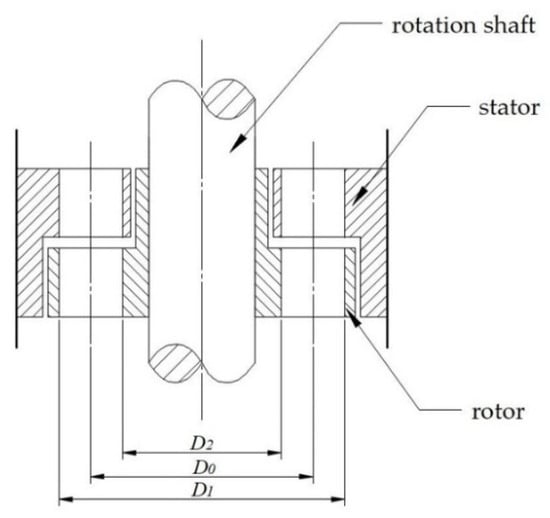
Figure 1.
Schematic diagram of the axial-flow turbine structure.
Key parameters involved in the design of turbine blades include the flow path’s outer diameter , inner diameter width , blade axial height , radial height , chord length , pitch , number of blades , rotor inlet structural angle , rotor outlet structural angle , stator inlet structural angle , stator outlet structural angle , and blade installation angle , as illustrated in Figure 2.
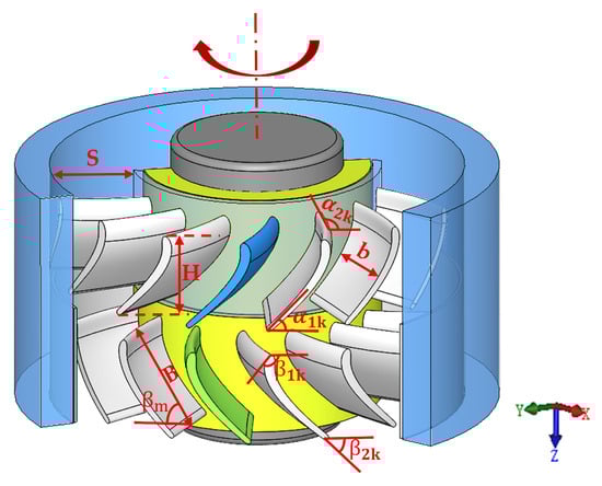
Figure 2.
Schematic diagram of parameters required for turbine blade design.
The Φ73 mm turbine section, designed for use with a Φ114.3 mm PDC drill bit, is engineered for drilling pressures of 5 to 30 kN [19,20]. The shaft diameter is set at 30 mm with an external flow path diameter of 60 mm. To reduce manufacturing and installation difficulties and to minimize frictional losses on the blade exteriors, a 0.75 mm tip clearance is maintained between the rotor blades and the wheel rim [21], with an adjusted outer diameter of 58.5 mm.
Using the optimal operating conditions method, where the stator and rotor outlet fluid flow angles equal their respective structural outlet angles (i.e., ), along with dimensionless coefficients (axial velocity , impact degree coefficient , and circulation coefficient ), other turbine blade-shaping parameters are determined. It is important to note that due to the complexity of fluid flow within the turbine, the unit theory method is employed to simplify calculations, reducing the fluid motion to movement within a cylindrical layer of computational diameter . The relevant calculation formulas are as follows:
Computational diameter
Axial velocity ()
where the axial component of the fluid’s absolute velocity ; circumferential velocity ; contraction coefficient is 0.9; blade pitch ; represents effective flow; and b is the blade’s radial height.
Impact degree coefficient ma
where represents the fluid’s converted pressure head; and are the absolute velocities at the rotor’s inlet and outlet, respectively.
Circulation coefficient :
where and are the circumferential components of the absolute velocities at the rotor’s inlet and outlet, respectively.
From the Formulas (2)–(4), it is evident that the three dimensionless coefficients for turbine design are exclusively related to the turbine blade’s inlet and outlet structural angles. Following a detailed derivation, the specific relationships are as follows:
When the impact degree coefficient ma is 0.5, the blades of the stator and rotor are mirror-symmetrical, with , , which results in the highest operational efficiency for the turbine [22]. The basic structural parameters of the designed turbine are listed in Table 1.

Table 1.
Basic parameters of the turbine.
2.2. Three-Dimensional Modeling of the Turbine
After obtaining the necessary parameters for the single-stage turbine, a basic model was developed using three-dimensional modeling software. The leading and trailing edges of the blades are defined using Bezier curves. The designed three-dimensional model of the single-stage turbine is illustrated in Figure 3.
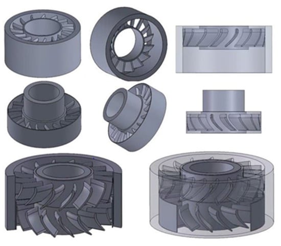
Figure 3.
Three-dimensional solid and perspective model of the single-stage turbine stator and rotor.
3. Turbine Section CFD Numerical Simulation
3.1. Turbulence Model
Among various turbulence models, the Shear Stress Transport () model is renowned for its superior accuracy and suitability for impeller machinery. This model combines the advantages of both the and models, addressing the dependency issues of the original model concerning free-stream values outside the boundary layer. Near the wall, the model is applied, whereas the model is used in the free stream [23,24,25].
Initially, the fundamental equations of the original model are as follows:
Transforming the high Reynolds number standard model equations into the model yields the following:
By multiplying (7) the Equation (9) by the blending function F1 and another set by (1 − F1), and combining them, the SST model equations are formulated as follows:
where the blending function F1 is set to 1 within the boundary layer and law-of-the-wall regions, gradually transitioning to 0 as it moves away from the boundary. The formula for F1 is
In this formula, y represents the distance to the nearest wall surface. .
Defining as the closure coefficients from the original model, , , , , , as those from the high Reynolds number standard model, and , , , , as those in the SST model, , β, , , γ the relationship is as follows:
The closure coefficients currently used are = 0.09, = 0.075, = 0.85, = 0.5, = /β* − k2/, = 0.0828, = 1.0, = 0.856, = / − k2/, k = 0.41.
3.2. Mesh Division and Flow Parameter Simulation Settings
To solve the numerical solutions for the flow-field parameters of the stator and rotor, the fluid domain is segmented into structured meshes, with densification near the wall surfaces. The grid size between neighboring grids grows from the wall in multiples of 1.2, with wall y+ around 1, locally greater than 1 but all less than 2. The inlet is set with a drilling fluid flow rate of 30 L/s, a plastic viscosity of 10 mPa·s, and the rotor’s rotational speed at 700 rpm, as illustrated in Figure 4.
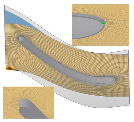
Figure 4.
Mesh division for single-stage turbine.
The number of meshes directly impacts the precision of simulation results. Validation under consistent boundary conditions with mesh counts of 500,000; 1,000,000; 2,000,000; and 3,000,000 was conducted to determine the optimal mesh count, assessing pressure drop, torque, and power (Figure 5).
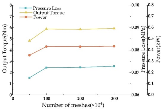
Figure 5.
Mesh independence analysis results.
Upon reaching 1,000,000 meshes, further increases result in negligible differences in the model’s torque, power, and pressure drop. The performance curves flatten, indicating that 1,000,000 meshes suffice for computational accuracy in subsequent simulations.
3.3. Programs for Numerical Simulation
Different cross-sections along the z-axis are chosen to evaluate the impact of blade parameters on the vortex structures within various turbine regions. The rotor is referred to as zone ‘a’, identified by cross-sections a01, a05, a10, a15, and a16; the stator is marked as zone ‘b’, with cross-sections b05, b10, b15, and b16 (Figure 6). Notably, b16 and a01 are situated at the stator outlet and rotor inlet, respectively.
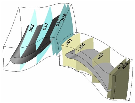
Figure 6.
Schematic of different cross-sections along the Z-axis of turbine stator and rotor.
To maximize the turbine’s hydraulic performance, the structural parameters of the blades should be kept within a reasonable range: (1) Drawing on extensive design and manufacturing experience, the optimal range for the leading-edge radius is 0.6–1.0 mm; (2) The ideal trailing-edge radius is between 0.3 and 0.6 mm; (3) Considering the overall length of the tool, turbines with different axial clearances of 2 mm, 4 mm, 6 mm, 8 mm, and 10 mm were designed; (4) This study designed a Φ73 mm turbine with 16 blades, and the staggered angles between the stator and rotor ranged from 0° to 22.5° (Figure 7), with angles of 0°, 4.5°, 9°, 13.5°, 18°, and 22.5° selected to simulate the impact of staggered installation angles on turbine performance.
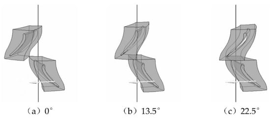
Figure 7.
Schematic of different installation staggered angles for turbine stator and rotor.
Different parameter values were set, and numerical simulations were carried out to compare the performance parameters such as output power, torque, and pressure drop of the turbine in the simulation results, in order to analyze the effect of each structural parameter on different parts of the turbine.
In summary, this paper presents a numerical simulation study of the parameters shown in Table 2.
Table 2.
Parameters of the study test.
4. Simulation Results and Discussion
4.1. Simulation Results Analysis
Figure 8a shows that as the leading-edge radius increases, the turbine’s torque, power, and pressure drop rise sharply between 0.6 and 0.7 mm and then stabilize between 0.7 and 1.0 mm, with the pressure drop slightly decreasing thereafter. Figure 8b demonstrates that both turbulence vortex dissipation and turbulence kinetic energy increase initially, then decrease, and stabilize after 0.8 mm.
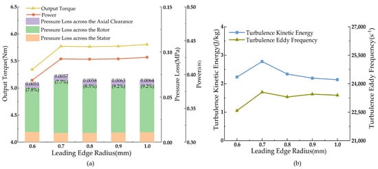
Figure 8.
Single-stage turbine performance parameters with changes in leading-edge radius. (a) Plot of torque, pressure drop, and power versus leading-edge radius; (b) Curve of turbulent kinetic energy and turbulent eddy frequency versus leading-edge radius.
According to the Q-criterion defined in [26], regions with values greater than zero in the cloud diagram are predominantly influenced by vortices, while negative values indicate dominance by strain rates or viscous stresses. Figure 9 reveals that the vorticity distribution on the pressure surface of the turbine rotor remains largely unchanged with variations in the leading-edge radius, while irregular changes occur on the suction side, particularly at 0.7 mm where the vortex-affected area is more concentrated and the vorticity is higher, leading to a less stable internal flow field in the turbine. This instability also explains the fluctuations observed in Figure 7. From 0.8 to 1.0 mm, the vortex groups on the lower part of the rotor blade suction side are smaller and more dispersed, with gradually increasing vortex influence. The increase in the leading-edge radius has minimal impact on the stator’s vortex structure (Figure 10).
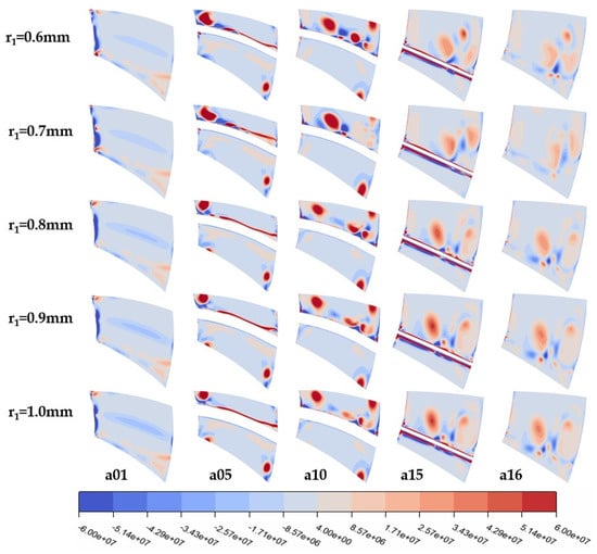
Figure 9.
Q-criterion cloud diagrams at different leading-edge radii of turbine rotor at various cross-sections.
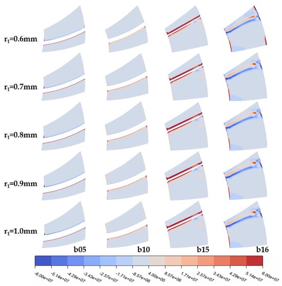
Figure 10.
Q-criterion cloud diagrams at different leading-edge radii of turbine stator at various cross-sections.
Simulation results suggest that turbine performance stabilizes after a leading-edge radius of 0.8 mm, achieving a pressure drop of 0.0688 MPa. The stator experiences the smallest pressure drop, indicating minimal non-useful pressure loss during turbine operation [27], with an output power of 0.423 kW and output torque of 5.764 Nm, meeting the design specifications.
Similarly, the trailing-edge radius should not be excessively large to avoid pronounced trailing vortex effects at the turbine blade outlet, which could lead to excessive hydraulic losses. As the trailing-edge radius increases, the turbine’s torque, power, pressure drop, turbulence kinetic energy, and turbulence vortex dissipation rate all continuously rise (Figure 11), due to the increased wake caused by a larger trailing-edge radius, which induces resistance leading to increased turbine pressure drops, as well as increased turbulence kinetic energy and more complex, disordered turbulent motion; thereby, increasing vortex dissipation.
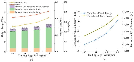
Figure 11.
Single-stage turbine performance parameters with changes in trailing-edge radius. (a) Plot of torque, pressure drop, and power versus trailing-edge radius; (b) Curve of turbulent kinetic energy and turbulent eddy frequency versus trailing-edge radius.
The increase in trailing-edge radius impacts the vortex structures in the flow domain near the rotor, as depicted in Figure 12. With an increase in trailing-edge radius, the vortex-affected areas at the turbine rotor inlet hub, outlet, and blade-suction side gradually expand, and the vortex intensity strengthens; the pressure surface is less influenced by vortices, although the overall vortex-affected area enlarges. The effect on the stator is concentrated at the tail (Figure 13), with no significant vortex region changes at the stator inlet and upper middle parts, but the tail and outlet areas are increasingly influenced by vortices with a larger trailing-edge radius.
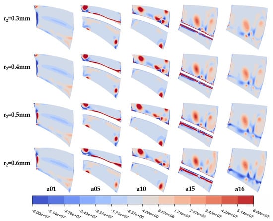
Figure 12.
Q-criterion cloud diagrams at different trailing-edge radii of single-stage turbine rotor interface.
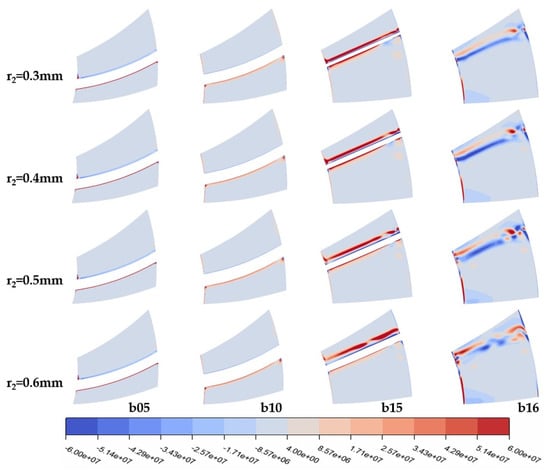
Figure 13.
Q-criterion cloud diagrams at different trailing-edge radii of single-stage turbine stator at various cross-sections.
At a trailing-edge radius of 0.4 mm, the pressure drop is 0.0716 MPa, the output power is 0.430 kW, and the output torque is 5.865 Nm. Compared to 0.3 mm, the output performance is better, and compared to 0.5 mm and 0.6 mm, the turbulence vortex dissipation rate is significantly lower, the fluid flow is more stable, and the losses are less.
Setting a reasonable axial clearance for the turbine stator and rotor ensures the free rotation of the rotating system and prevents damage from collisions between the stator and rotor. Axial clearance is very important for the lifespan of the drilling tool.
From Figure 14a, within the axial clearance range of 2–6 mm, the output torque, pressure drop, and power of the turbine first increase and then decrease, with all three parameters remaining essentially unchanged after 6 mm. According to Figure 14b, the turbine’s turbulence kinetic energy increases in a parabolic manner with increasing axial clearance, then decreases, while the turbulence vortex dissipation rate linearly decreases. This is because, as the axial clearance increases, the influence of the turbine rotor movement on the development of the stator wake decreases, reducing the generation of large energy vortex groups; thereby, decreasing vortex dissipation.
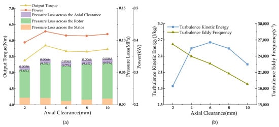
Figure 14.
Single-stage turbine performance parameters with changes in axial clearance. (a) Plot of torque, pressure drop, and power versus axial clearance; (b) Curve of turbulent kinetic energy and turbulent eddy frequency versus axial clearance.
As shown in Figure 15, changes in axial clearance have a significant impact on the vortex structures near the stator tail and the overall rotor. In the vorticity cloud diagrams, the red areas are positive (velocity vectors in the counterclockwise direction), and the blue areas are negative. The larger the vorticity, the faster the fluid microgroups rotate around their center, the more severe the disturbance in the flow field, and the more likely flow separation occurs. As the axial clearance increases, the intensity of the vortices on the stator wake and the rotor pressure surface gradually weakens, the positive vorticity area on the rotor suction side gradually increases while the negative area decreases, and the mixing process of the upstream wake with the mainstream lengthens with increasing axial clearance; thereby, enhancing the uniformity of fluid-flow parameters. From the Q-criterion cloud diagrams, the throat and tail of the rotor-suction side are mainly influenced by vortices, the affected area gradually decreases, and the high-vorticity area also decreases. The smaller the axial gap, the greater the impact of the turbine rotor’s rotation on the turbine stator’s tail, and the more unstable the fluid-motion state.
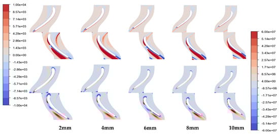
Figure 15.
Q-criterion cloud diagrams and vorticity of single-stage turbine stator and rotor at different axial clearances.
With an axial clearance of 6 mm, the single-stage turbine’s pressure drop is 0.067 MPa, output power is 0.416 kW, and output torque is 5.671 Nm, with the lowest dissipation rate and highest turbulence kinetic energy, making it the optimal output performance for the turbine.
As shown in Figure 16, simulation results indicate that changes in staggered angles result in minimal variations in the turbine’s output pressure drop, torque, and power, with the turbine’s output performance remaining essentially stable within a cycle. The impact of different installation-staggered angles on turbine performance is negligible.
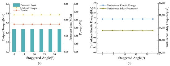
Figure 16.
Single-stage turbine performance parameters with changes in installation-staggered angles for turbine stator and rotor. (a) Plot of torque, pressure drop, and power versus staggered angles; (b) Curve of turbulent kinetic energy and turbulent eddy frequency versus staggered angles.
Based on the simulation results, the turbine’s optimal shaping parameters are determined with a leading-edge radius of 0.8 mm, a trailing-edge radius of 0.4 mm, and an axial clearance of 6 mm, providing the best relative output performance for the designed Φ73 mm single-stage turbine. The staggered angle does not alter the turbine’s output performance; once the structural parameters of the turbine are established, there is no need to consider the consistency of staggered angles during assembly.
4.2. Discussion
Initially, the output performance curve of the φ73 mm single-stage turbine was validated (Figure 17) to assess its rationality. This curve, representing water as the fluid medium at a flow rate of 30 L/s, illustrates a clear linear relationship between the turbine’s output torque and rotational speed, with torque decreasing as speed increases. The designed single-stage turbine achieves a braking torque of 6.5 Nm; the power increases initially then decreases with rising speed, peaking at 1.17 kW at 3500 rpm; hydraulic efficiency follows a similar trend; pressure drop changes minimally with speed. The turbine performance prediction curve simulation aligns with the theoretical characteristics of turbine drilling tools, validating the turbine’s design.
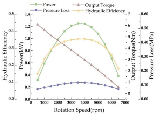
Figure 17.
Performance validation curve for single-stage turbine.
In order to verify the reliability of the simulations used in the study, the results of this paper are compared with existing well-established conclusions. According to Verhaagen et al. [28] a larger leading-edge radius reduces the size and strength of the main vortex and moves the main vortex outward, which is consistent with the effect of the leading-edge radius on the interior of the turbine in this study. Similarly to the study by Yun et al. [15], the trailing-edge profile has a greater effect on the mechanical properties of the impeller than other parameters, and an increase in trailing-edge radius increases the turbine output power. The study of Yamada et al. [29] confirmed that the efficiency of the turbine changed nonlinearly with the increase in axial clearance. In addition to this, according to Busby et al. [30], as the axial clearance decreases, the stator-rotor interaction is enhanced as well as the wake mixing losses are reduced, leading to an increase in stator losses. This corroborates the conclusions drawn from the study in this paper.
In addition to this, the paper refers to the study of Gong et al. [31]. According to the modeling parameters in [31], the same model is established, and the simulation method used in this study is applied to set the same boundary conditions to simulate the vortex structure in the second-stage turbine stator at an inlet attack angle of 0° and a rotational speed of 3000 rpm, and the results are compared with the experiments in the references, as shown in Figure 18. Based on the results of the comparison, it can be seen that the output of the vortex structure cloud diagrams of the simulation method used in this paper is similar to that of the vortex structure observed in the experiments. Thus, the simulation method used in this paper is feasible and the simulation results are reliable.
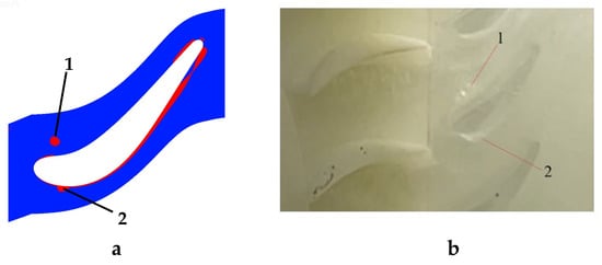
Figure 18.
Simulation method validation. (a) Output pictures of the simulation scheme in this paper; (b) Experimental results of Ref.
5. Turbine Performance Prediction
5.1. Turbine Output Performance Prediction at Different Speeds
To determine the turbine’s output performance at low speeds, simulations were performed from 0 to 200 rpm, with results shown in Figure 19. At low speeds, the turbine’s power and hydraulic efficiency, compared to pressure drop and torque, are significantly more affected by speed, showing a linear increase. The pressure drop remains almost unchanged, under 0.04 MPa; torque slightly decreases with increasing speed, reaching over 6.3 Nm; power achieves up to 0.1 kW.
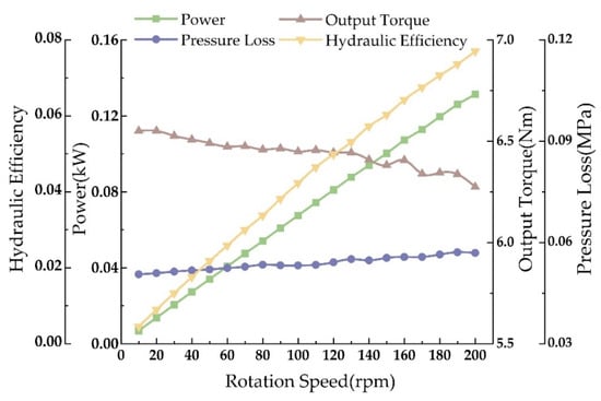
Figure 19.
Turbine performance prediction curve at low speeds.
5.2. Turbine Output Performance Prediction at Different Displacements
Simulations were conducted for single-stage turbines at flow rates ranging from 10 to 30 L/s, with results depicted in Figure 20. With increasing displacement, the power, torque, and pressure drop of the turbine all increase at a given speed, with a progressively larger increment. Under conditions approximating actual operational low speeds and small displacements, the single-stage turbine’s pressure drop is controlled below 0.007 MPa, torque exceeds 0.8 Nm, and power reaches 0.01 kW.
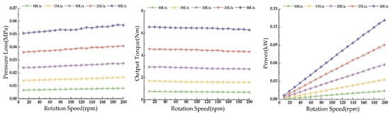
Figure 20.
Turbine performance prediction curve at different displacements.
5.3. Turbine Output Performance Prediction at Different Fluid Viscosities
At a drilling site, drilling fluid viscosity varies. Simulations for fluid viscosities ranging from 5 to 30 mPa·s were conducted at a flow rate of 10 L/s and a speed of 80 rpm (Figure 21). The results demonstrate that the turbine’s torque, power, and pressure drop all increase with rising fluid viscosity. The effect on pressure drop is particularly significant, with increased viscosity substantially raising the turbine’s pressure losses, thereby reducing its operational efficiency. Under these conditions, the single-stage turbine’s output torque can reach up to 1.6 Nm.
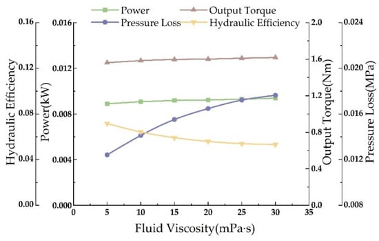
Figure 21.
Turbine performance prediction curve at different fluid viscosities.
6. Conclusions
Based on CFD methods, numerical simulations were performed on the designed φ73 mm turbine drill section, yielding optimal assembly and shaping parameters for the single-stage turbine, and evaluating performance under different speeds, displacements, and fluid viscosities. The findings are as follows:
- (1)
- The calculated inlet and outlet structural angles for the designed turbine blades are, respectively, 120° and 55.7°, with an installation angle of 55°, a blade radial height of 12 mm, a chord length of 13 mm, and a blade count of 16. The leading-edge radius is established at 0.8 mm, the trailing-edge radius at 0.4 mm, and the axial clearance at 6 mm.
- (2)
- When the radius of the leading edge is within the range of 0.8–1.0 mm and the axial clearance is within the range of 6–10 mm, the performance of the turbine’s output torque, pressure drop, and power fluctuates within the range of 0.1–0.5%, and the output performance remains stable. Variations in the staggered angles of the stator and rotor assembly have minimal impact on output performance, in one rotation cycle; regardless of the initial stator–rotor installation staggering angle, the turbine output performance fluctuation is less than 0.02%. Pressure drop, torque, power, turbulence kinetic energy, and turbulence vortex dissipation rate all increase with an increasing trailing-edge radius.
- (3)
- The impact of the leading-edge radius on the turbine’s internal flow field is irregular, concentrated on the rotor’s suction side, and virtually negligible on the stator. Changes in the trailing-edge radius and axial clearance systematically influence the flow fields of both the entire rotor and the middle to rear parts of the stator. As the trailing-edge radius increases, the vortex-affected region of the turbine rotor as a whole as well as the stator tail expands, and the flow is unstable; in contrast, the larger the axial clearance is, the smaller the vortex-affected region inside the turbine is, and the more stable the flow is. The trailing-edge radius of the blade has a more pronounced effect on turbine performance compared to other parameters. With the increase in trailing-edge radius, each output performance of the turbine is increasing, and the increase is becoming larger and larger, without a tendency to stabilize.
- (4)
- Predictions for turbine performance under conditions of low speed, low displacement, and high fluid viscosity resulted in a controlled output pressure drop below 0.018 MPa, with torque reaching 1.6 Nm. Utilizing 100–200 stage turbines as the power device, an expected output torque of 150–300 Nm could be achieved, sufficient to meet the demands for small-hole window sidetracking and rock-breaking.
Author Contributions
X.L., Y.T. and Q.H. developed a hydrodynamic model of a turbine rig blade. X.S., Y.T. and C.D. conceived and designed the simulation and wrote the paper. All authors have read and agreed to the published version of the manuscript.
Funding
This work is supported by the National Natural Science Foundation of China (No. 52374007).
Data Availability Statement
The original contributions presented in this study are included in the article. Further inquiries can be directed to the corresponding author.
Acknowledgments
We sincerely acknowledge the former researchers for their excellent work, which greatly assisted our academic study.
Conflicts of Interest
Author Xianyi Li is employed by the Beijing Petroleum Machinery Co.; The remaining authors declare that the research was conducted in the absence of any commercial or financial relationships that could be construed as a potential conflict of interest.
References
- Wang, H.; Huang, H.; Bi, W.; Ji, G.; Zhou, B.; Zhuo, L. Deep and ultra-deep oil and gas well drilling technologies: Progress and prospect. Nat. Gas Ind. B 2022, 9, 141–157. [Google Scholar] [CrossRef]
- Geissler, N.; Garsche, F.; Samus, V.; Polat, B.; Di Mare, F.; Bracke, R. Proof of Concept in a Full-Scale Field Test for the Novel Micro-Turbine Drilling Technology from a Cased Borehole in Granite Rock. SPE J. 2024, 1–9. [Google Scholar] [CrossRef]
- He, Y.; Wang, Y.; Zhang, D.; Xu, Y. Optimization design for turbodrill blades based on a twisting method. J. Pet. Sci. Eng. 2021, 205, 108892. [Google Scholar] [CrossRef]
- Mokaramian, A.; Rasouli, V.; Cavanough, G. CFD Simulations of Turbodrill Performance with Asymmetric Stator and Rotor Blades Configuration; CSIRO: Melbourne, Australia, 2012; pp. 10–12.
- Yu, W.; Yao, J.Y.; Li, Z.J. Design and Development of Turbodrill Blade Used in Crystallized Section. Sci. World J. 2014, 2014, 682963. [Google Scholar] [CrossRef]
- Mokaramian, A.; Rasouli, V.; Cavanough, G. Turbodrill Design and Performance Analysis. J. Appl. Fluid Mech. 2015, 8, 377–390. [Google Scholar] [CrossRef]
- Wang, Y.; Xia, B.; Wang, Z.; Wang, L.; Zhou, Q. Design and Output Performance Model of Turbodrill Blade Used in a Slim Borehole. Energies 2016, 9, 1035. [Google Scholar] [CrossRef]
- Seale, R.; Beaton, T.; Flint, G. Optimizing turbodrill designs for coiled tubing applications. In Proceedings of the SPE Eastern Regional Meeting, Charleston, WV, USA, 15–17 September 2004; p. SPE-91453-MS. [Google Scholar]
- Zhang, D.; Wang, Y.; Sha, J.; He, Y. Performance Prediction of a Turbodrill Based on the Properties of the Drilling Fluid. Machines 2021, 9, 76. [Google Scholar] [CrossRef]
- Geissler, N.; Garsche, F.; di Mare, F.; Bracke, R. Overview and comprehensive performance description of a new Micro Turbine Drilling—MTD technology for drilling laterals into hard reservoir rock. Int. J. Rock Mech. Min. Sci. 2023, 161, 105253. [Google Scholar] [CrossRef]
- Yan, Z.; Zhao, X.; Pan, W.; Wang, Z.; Chen, Z.; Wang, H. Mechanism analysis and CFD investigation on the key structures of the guide wheel and turbine for a high-power turbine generator while drilling. Geoenergy Sci. Eng. 2025, 246, 213609. [Google Scholar] [CrossRef]
- Song, C.; Wu, G.; Zhu, W.; Zhang, X.; Zhao, J. Numerical Investigation on the Effects of Airfoil Leading Edge Radius on the Aerodynamic Performance of H-Rotor Darrieus Vertical Axis Wind Turbine. Energies 2019, 12, 3794. [Google Scholar] [CrossRef]
- Davandeh, N.; Maghrebi, M.J. Leading Edge Radius Effects on VAWT Performance. J. Appl. Fluid Mech. 2023, 16, 1877–1886. [Google Scholar] [CrossRef]
- Fadilah, P.A.; Hartono, F.; Erawan, D.F. Effect of impeller trailing edge shape to the radial compressor performance. AIP Conf. Proc. 2020, 2248, 030005. [Google Scholar]
- Yun, J.-E.; Atac, O.F.; Kim, J.-B.; Kim, G.-Y. Influence of trailing edge curve on the performance of radial turbine in turbocharger. Int. J. Low-Carbon Technol. 2023, 18, 570–579. [Google Scholar] [CrossRef]
- Grönman, A.; Turunen-Saaresti, T.; Röyttä, P.; Jaatinen-Värri, A. Influence of the axial turbine design parameters on the stator–rotor axial clearance losses. Proc. Inst. Mech. Eng. Part A J. Power Energy 2014, 228, 482–490. [Google Scholar] [CrossRef]
- Zhang, X. Effect of Axial Clearance Between Turbine and Guide Wheel on Hydraulic Performance of Mine Borehole Turbo Generator. J. Phys. Conf. Ser. 2024, 2860, 012006. [Google Scholar] [CrossRef]
- Bardina, J.E.; Huang, P.G.; Coakley, T.J. Turbulrnce Modeling Validation. In Proceedings of the 28th Fluid Dynamics Conference, Snowmass Village, CO, USA, 29 June–2 July 1997. [Google Scholar] [CrossRef]
- Li, W.; Chen, J.; Wang, Y. Development status of drilling technology of small borehole wells at home and abroad. Nat. Gas Ind. 2009, 29, 54–56+63+136–137. [Google Scholar]
- Zhong, H. Research and application of drilling and completion technology of horizontal wells with ultra-short radius sidetrack drilling. West. Explor. Eng. 2023, 35, 37–40. [Google Scholar]
- Chapman, J.W.; Guo, T.-H.; Kratz, J.L.; Litt, J.S. Integrated Turbine Tip Clearance and Gas Turbine Engine Simulation. In Proceedings of the 52nd AIAA/SAE/ASEE Joint Propulsion Conference, Salt Lake City, UT, USA, 25–27 July 2016. [Google Scholar]
- Wan, B.; Li, J. Petroleum Engineering Fluid Machinery, 1st ed.; Petroleum Industry Press: Beijing, China, 1999; pp. 213–240. [Google Scholar]
- Wu, B. CFD investigation of turbulence models for mechanical agitation of non-Newtonian fluids in anaerobic digesters. Water Res. 2011, 45, 2082–2094. [Google Scholar] [CrossRef] [PubMed]
- Menter, F.R. Two-equation eddy-viscosity turbulence models for engineering applications. AIAA J. 1994, 32, 1598–1605. [Google Scholar] [CrossRef]
- Yang, J.; Wu, H. Explicit coupled solution of double square k-ωSST turbulence model and its application to impeller machinery. J. Aeronaut. 2014, 35, 116–124. [Google Scholar]
- Zhan, J.-M.; Li, Y.-T.; Wai, W.-H.O.; Hu, W.-Q. Comparison between the Q criterion and Rortex in the application of an in-stream structure. Phys. Fluids 2019, 31, 121701. [Google Scholar] [CrossRef]
- Mokaramian, A.; Rasouli, V.; Cavanough, G. Fluid Flow Investigation through Small Turbodrill for Optimal Performance. Mech. Eng. Res. 2013, 3, 1–24. [Google Scholar] [CrossRef]
- Verhaagen, N.G. Leading-Edge Radius Effects on Aerodynamic Characteristics of 50-Degree Delta Wings. J. Aircr. 2012, 49, 521–531. [Google Scholar] [CrossRef]
- Yamada, K.; Funazaki, K.-i.; Kikuchi, M.; Sato, H. Influences of axial gap between blade rows on secondary flows and aerodynamic performance in a turbine stage. In Proceedings of the Turbo Expo: Power for Land, Sea, and Air, Orlando, FL, USA, 8–12 June 2009; pp. 1039–1049. [Google Scholar]
- Busby, J.A. Influence of Vane-Blade Spacing on Transonic Turbine Stage Aerodynamics, Part 2: Time-Resolved Data and Analysis. Asme Pap. 1999, 21, 637–682. [Google Scholar] [CrossRef]
- Gong, Y.; Liu, Y.; Wang, C.; Zhang, J.; He, M. Investigation on Secondary Flow of Turbodrill Stator Cascade with Variable Rotary Speed Conditions. Energies 2023, 17, 162. [Google Scholar] [CrossRef]


Disclaimer/Publisher’s Note: The statements, opinions and data contained in all publications are solely those of the individual author(s) and contributor(s) and not of MDPI and/or the editor(s). MDPI and/or the editor(s) disclaim responsibility for any injury to people or property resulting from any ideas, methods, instructions or products referred to in the content. |
© 2025 by the authors. Licensee MDPI, Basel, Switzerland. This article is an open access article distributed under the terms and conditions of the Creative Commons Attribution (CC BY) license (https://creativecommons.org/licenses/by/4.0/).