Abstract
The layout of acoustic emission sensors plays a critical role in non-destructive structural testing. This study proposes a grid-based optimization method focused on multi-source location results, in contrast to traditional sensor layout optimization methods that construct a correlation matrix based on sensor layout and one source location. Based on the seismic source travel time theory, the proposed method establishes a location objective function based on minimum travel time differences, which is solved through the particle swarm optimization (PSO). Furthermore, based on location accuracy across various configurations, the method systematically evaluates potential optimal sensor locations through grid search. Synthetic tests and laboratory pencil-lead break (PLB) experiments are conducted to compare the effectiveness of PSO, genetic algorithm (GA), and simulated annealing (SA), with the following conclusions. (1) In the synthetic tests, the proposed method achieved an average location error of 1.78 mm, outperforming that based on the traditional layout, GA and SA. (2) For different noise cases, the location accuracy separately improved by 24.89% (σ = 0.5 μs), 12.59% (σ = 2 μs), and 15.06% (σ = 5 μs) compared with the traditional layout. (3) For the PLB experiments, the optimized layout achieved an average location error of 9.37 mm, which improved the location accuracy by 59.15% compared with the traditional layout.
1. Introduction
Acoustic emission (AE) is a phenomenon where strain energy is released as transient elastic waves, which occur when a material experiences localized plastic deformation or crack formation [1]. AE monitoring technology is an effective non-destructive monitoring method. It captures elastic wave sensors [2] and allows for the determination of AE source location, source mechanism, and structural velocity. The sensor layout in an AE monitoring system is crucial for ensuring parameters high-precision inversion [3]. Therefore, it is necessary to develop an optimization method for the sensor network layout.
Early sensor layouts were determined based on personal experience. As a result, the sensor locations were highly subjective and often led to inaccurate results. In 1977, Kijko [4,5] proposed a D-value model for microseismic sensor layout optimization. This model determines the optimal sensor configuration by minimizing the determinant of the covariance matrix of source locations and travel times. Due to its flexibility, this method has been widely applied in the design of sensor network layouts. In 1990, Rabinowitz and Steinberg [6] introduced the DETMAX method, which improved the D-value model by preventing two sensors at the same location. Although the D-value model provides evaluation criteria for sensor layout design, it has some limitations. When the number of sensors is large, the model cannot cover all sensors and involves complex calculations. With the development of optimization algorithms, researchers have attempted to integrate these algorithms into sensor layout optimization. For example, by employing genetic algorithms (GA) for sensor layout optimization, Jones [7] proposed an optimal three-dimensional microseismic monitoring network based on arbitrarily shaped cavities. In 2013, Kraft et al. [8] proposed a regional-scale microseismic monitoring network optimization method based on simulated annealing (SA) and the D-value optimization criterion. This method can determine the geometry of a monitoring network that meets specified requirements. In 2014, Rosa-Cintas et al. [9] proposed a method to optimize seismic noise array measurements. They experimentally studied the effects of different array geometries and numbers of sensors on the relationship between seismic wave velocity and frequency, achieving a reliable relationship between seismic wave velocity and frequency with a limited number of sensors. In 2020, De Landro et al. [10] proposed an optimization method for monitoring networks integrated with small-scale seismic arrays. This method addressed the issue of high location errors associated with traditional surface station layouts in monitoring industrial-induced microseismic events. In 2022, Zhou et al. [11] proposed an optimization method for microseismic monitoring networks based on the S-V-E-R-V model. This method effectively addressed the issues of slow response speed and poor dynamic adaptability in traditional monitoring networks. In the same year, Li et al. [12] based on the arrival time difference principle and hyperbolic/hyperbolic control equations, revealed the influence mechanism of sensor network layout on MS/AE source location, proposed the principle of optimizing sensor network layout, and effectively improved the accuracy and stability of source location.
In summary, current sensor layout optimization primarily involves constructing an information matrix based on sensor positions and source location results. Optimization algorithms are then applied to the matrix to obtain the optimized sensor layout. However, these approaches entail significant complexity and limited flexibility for adjustment. Therefore, the optimized sensor layout computation can be shifted to directly reduce source location errors, which can simplify the overall process and improve computational efficiency.
The focus is now placed on reducing AE location errors. To achieve this, the key lies in employing more advanced methods to solve the objective function for source location. The commonly used methods currently include gradient descent approaches, such as Newton’s iteration and the simplex method [13,14], as well as heuristic methods including GA [15], particle swarm optimization (PSO) [16], and SA [17]. Gradient descent approaches are highly dependent on local derivative information and require highly accurate traditional values. In contrast, heuristic methods do not rely on derivative information and are less likely to become trapped in local optima. As a result, these methods are widely applied to solve the objective function in source location problems [18]. Among various heuristic algorithms, the PSO algorithm has been widely applied in geophysical inversion [19]. This algorithm is based on swarm intelligence and exhibits strong global optimization capabilities. For example, Chen et al. [20] proposed a microseismic source location method based on PSO and a layered velocity model, which achieved high location accuracy.
In summary, many existing algorithms can be tried for the earthquake source location and further optimization of sensor layout. However, existing sensor layout optimization methods often apply optimization algorithms directly to sensor layout optimization. To address this, the study proposes an optimization method for sensor layout based on the minimization of travel time differences. This study’s main innovations and contributions are as follows: (1) proposing a minimum travel-time-difference-based objective function for source location. This integrates PSO and grid search to optimize sensor layout, which improves the efficiency of location and enhances the method’s interpretability. (2) Synthetic tests compared the proposed model with GA and SA. The proposed method improved location accuracy by 7.81% compared to GA and by 7.39% compared to SA algorithms. (3) For different noise conditions, the proposed method improved location accuracy by 24.89% (σ = 0.5 μs), 12.59% (σ = 2 μs), and 15.06% (σ = 5 μs) compared to the traditional layout. These results demonstrate that the proposed method can maintain effective layout optimization under noise interference. (4) In laboratory AE pencil-lead break (PLB) experiments, the proposed method improved location accuracy by 59.15% compared to the traditional layout. It also achieved improvements of 32.18% and 20.48% compared to the GA and the SA algorithms, respectively.
2. Methodology
2.1. Sensor Location Objective Function
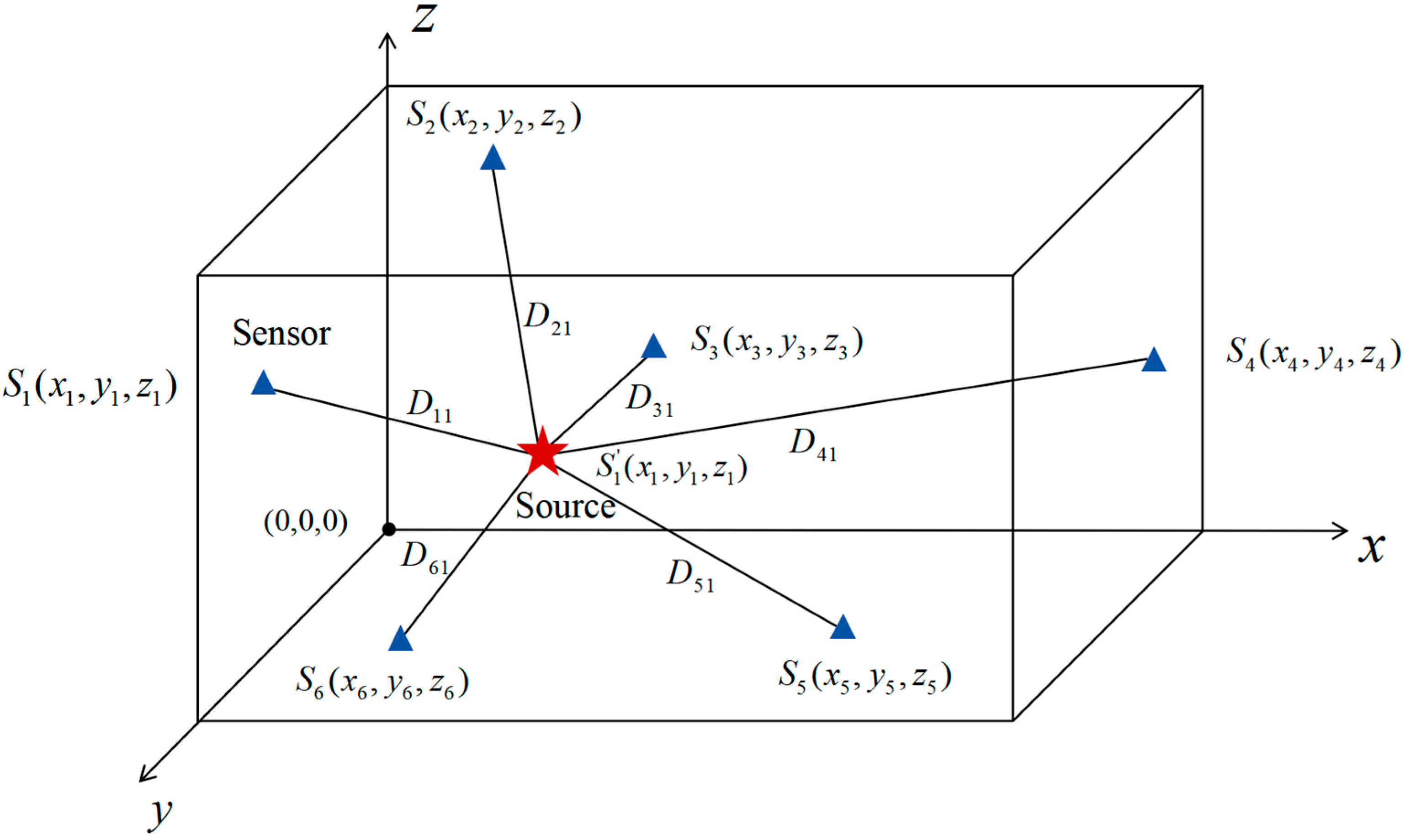
Assume that the sample where AE events occur is isotropic. In this case, signals from AE sources propagate linearly through the medium at a constant velocity. Assume that the sample where AE events occur is isotropic. In this case, signals from AE sources propagate linearly through the medium at a constant velocity. Assume that the P-wave velocity is , the coordinates of the AE sources and sensors shown in Figure 1 are and the sensor is , respectively.
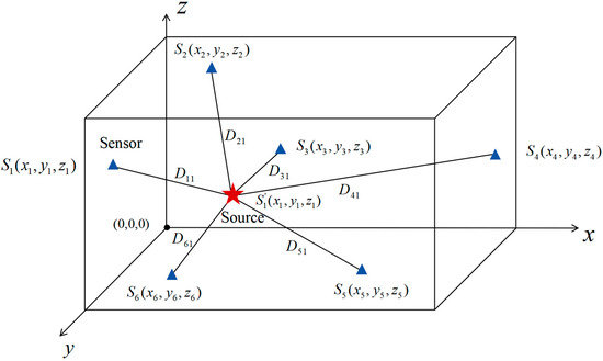
Figure 1.
Schematic diagram of the AE event and sensor locations.
Then, the distance between the AE source and sensor can be expressed as
where represents the sensor id, and denotes the AE event id. Furthermore, based on Equation (1), the travel time fitting error between the sensor and the AE source can be expressed as
where represents the actual travel time for the distance between sensor and AE source .
From Equation (2), it can be observed that the closer is to zero, the more accurate the location result of the AE source. Therefore, the location problem can be transformed into an optimization problem:
Therefore, the optimal AE source location can be determined by solving Equation (3). The following section will introduce how to solve Equation (3) by using the PSO algorithm.
2.2. PSO-Based Location Algorithm
PSO can efficiently search for the global optimum, which is suitable for solving complex problems. With the simple modeling and ease of implementation, PSO has been widely used in AE event location. In this study, we employed PSO to solve the location objective function based on minimum travel-time-difference-based Equation (3). The algorithm finds the optimal solution by simulating collaboration in a flock, initializing random solutions and iteratively updating each particle’s location and velocity. Each particle’s movement is determined by its personal best location and the swarm’s global best location, and then the trajectory is adjusted to locate the optimal solution. The specific steps of the PSO algorithm are as follows:
- Parameter initialization: Multi-particles are randomly generated, and each particle represents a potential AE event location. Each particle is assigned a random velocity and location , where represents the index of different particles.Then, these initial parameters of each particle are substituted into the objective function Equation (3) to calculate the initial fitness , which is then set as each particle’s personal best .
- Velocity and location update: The velocity of each particle is updated according to Equation (4):where represents the velocity of particle at time , and is set to 30; is the inertia weight, which determines the particle’s tendency to maintain its current velocity; is the velocity of particle at time ; and separately are learning factors that control the particle’s attraction to its personal best and the global best location, and they are both set to 1.49; and are random numbers within the range [0, 1].Then, the particle’s location is updated based on the updated velocity:where represents the location of particle at time , and is the location of particle at time .
- Fitness evaluation: After updating each particle’s location , the parameters represented by this location are substituted into the objective function . The is used to update the individual historical best location of particle at time and the global best location of the swarm.
- Updating and : The fitness function is used as a criterion, where lower values indicate higher accuracy in determining the optimal location. For each particle , if the new fitness is smaller than the fitness of its historical best location, the historical best location is updated as . Otherwise, the historical best location remains unchanged. Among the historical best locations of all particles, the location with the best fitness is selected as the global best location of the swarm. The updated equations are as follows:
- Iteration and convergence: By iteratively updating each particle’s velocity and location, updated and are generated until the maximum number of iterations is reached. Ultimately, the global best location is considered as the optimal coordinate for the AE event. This location represents the solution that minimizes the error of the objective function.
2.3. Sensor Layout Optimization Method
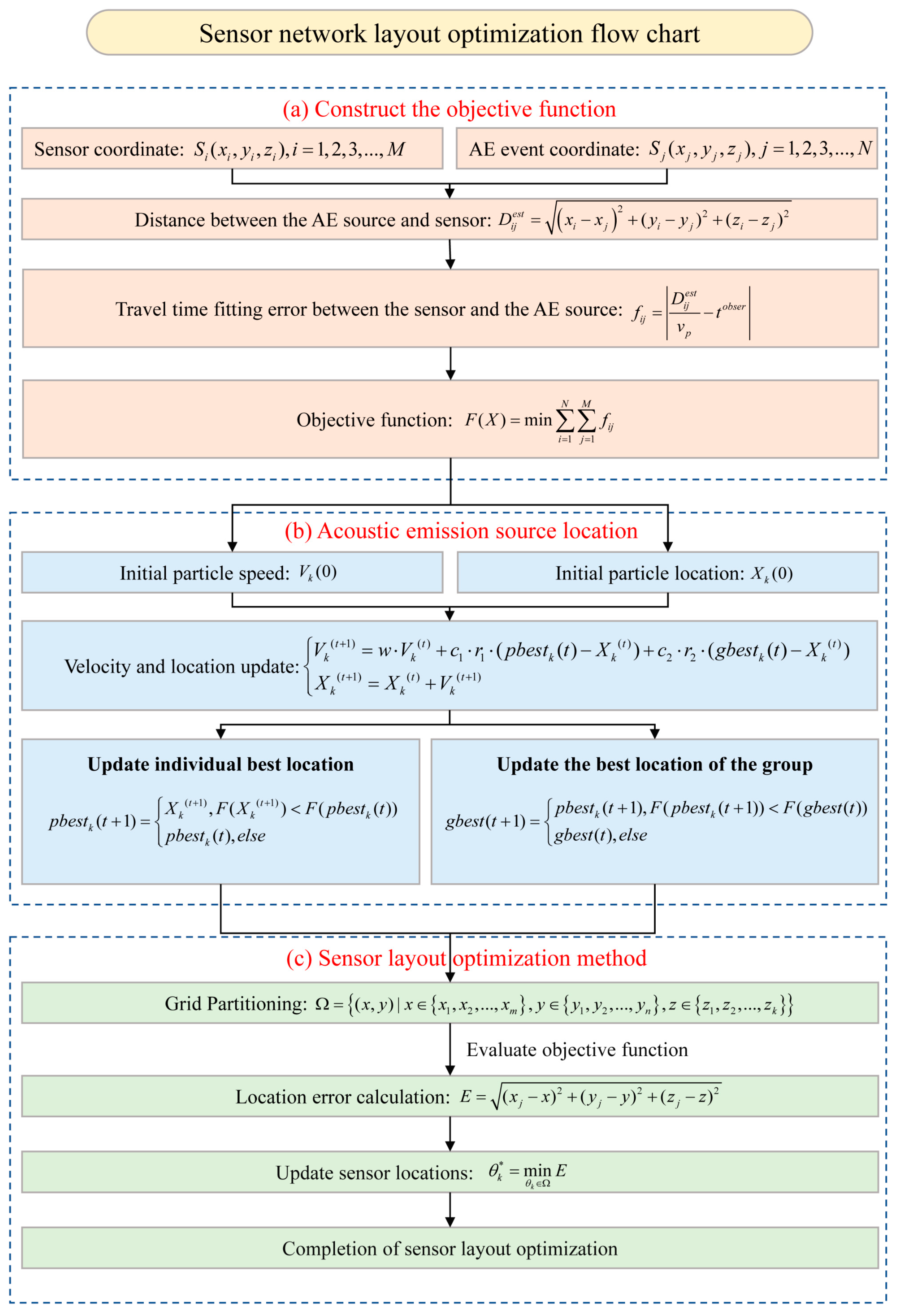
The PSO algorithm is used to evaluate the quality of the current sensor layout based on location errors of different sensor layouts. Sensor locations are adjusted step by step to reduce location errors. Grid search is a common approach in sensor optimization. By discretizing the search space into grid points, each possible location can be systematically evaluated. Raorane et al. [21] used a discretized square grid to determine the optimal location for a sensor cluster. Dong et al. [22] used rectangular grids with different aspect ratios to determine the optimal location of sensors. This approach not only provides a clear search space for the optimization algorithm, but also ensures accurate placement in experimental verification. This study applied a grid search method to iteratively change sensor locations and calculate location errors for different configurations to optimize the sensor layout. Figure 2 presents the overall process of the sensor layout optimization.
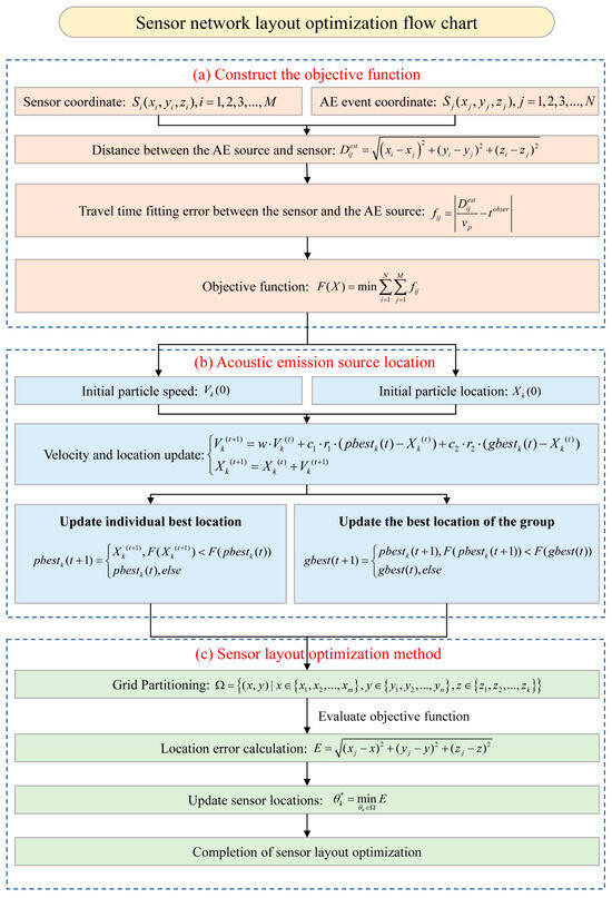
Figure 2.
Grid search optimization method for the sensor network layout.
- Grid Partitioning: Within the sensor deployment area, a regular grid is generated based on predefined spacing. The density of the grid points is determined by the required optimization accuracy. Assuming the target area is mm2, the set of grid points can be expressed aswhere , , and represent the coordinates of the grid points.
- Objective function evaluation: For each sensor , the location is moved to each candidate location . For each candidate location, the AE source location is calculated using Equation (3).
- Location error calculation: For each candidate location , the location error is calculated as the distance between the AE source location and the actual source location :where is the source location and is the actual source location.
- Update sensor locations: In each iteration, the candidate location with the minimum location error for each sensor is selected. This location is then updated as the new sensor layout configuration:If the error at this location is smaller than the current global minimum error , the global optimal location and the corresponding error are updated.
- Completion of sensor layout optimization: During the optimization process, the optimal sensor locations and the corresponding location errors for each iteration are recorded. The final optimization results are validated to ensure the rationality of the sensor layout and the improvement in location accuracy.
3. Synthetic Test
3.1. Sensor Network Optimization
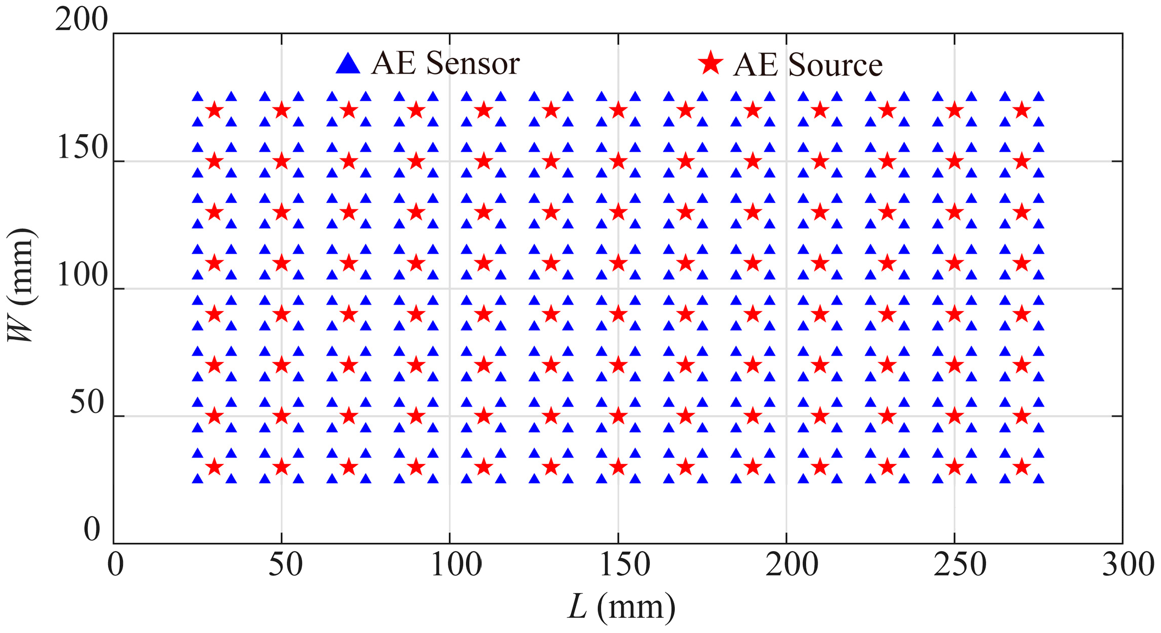
A sample with dimensions of 300 mm 200 mm was prepared. The P-wave velocity was set to = 6 km/s, and the standard deviation of the arrival time error was assumed to be σ = 0.5 μs. Many researchers have used 10 10 mm2 grids for PLB experiments [23]. Therefore, we set 10 10 mm2 as the unit grid. The grid intersection points were considered as potential sensor locations. To facilitate the implementation of subsequent indoor PLB experiments, we reserved a 25 mm margin around the rock sample. The potential sensors locations and the distribution of AE sources are shown in Figure 3.
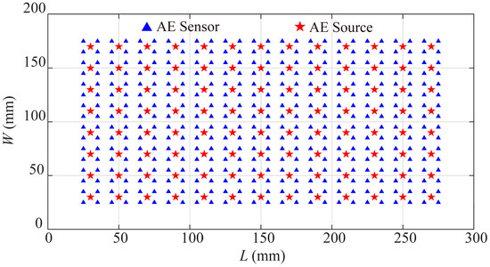
Figure 3.
Potential AE and sensor locations in the monitoring system.
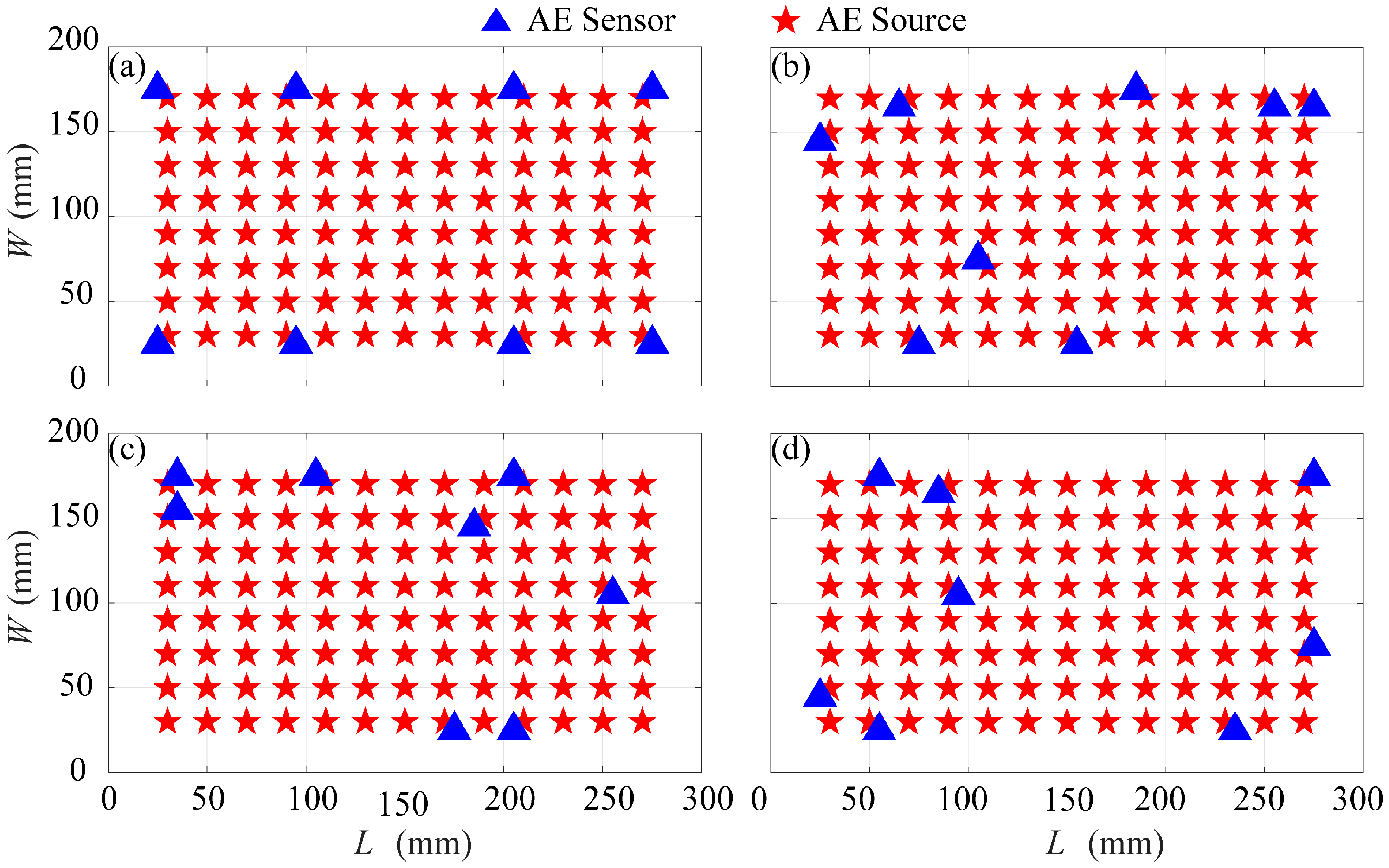
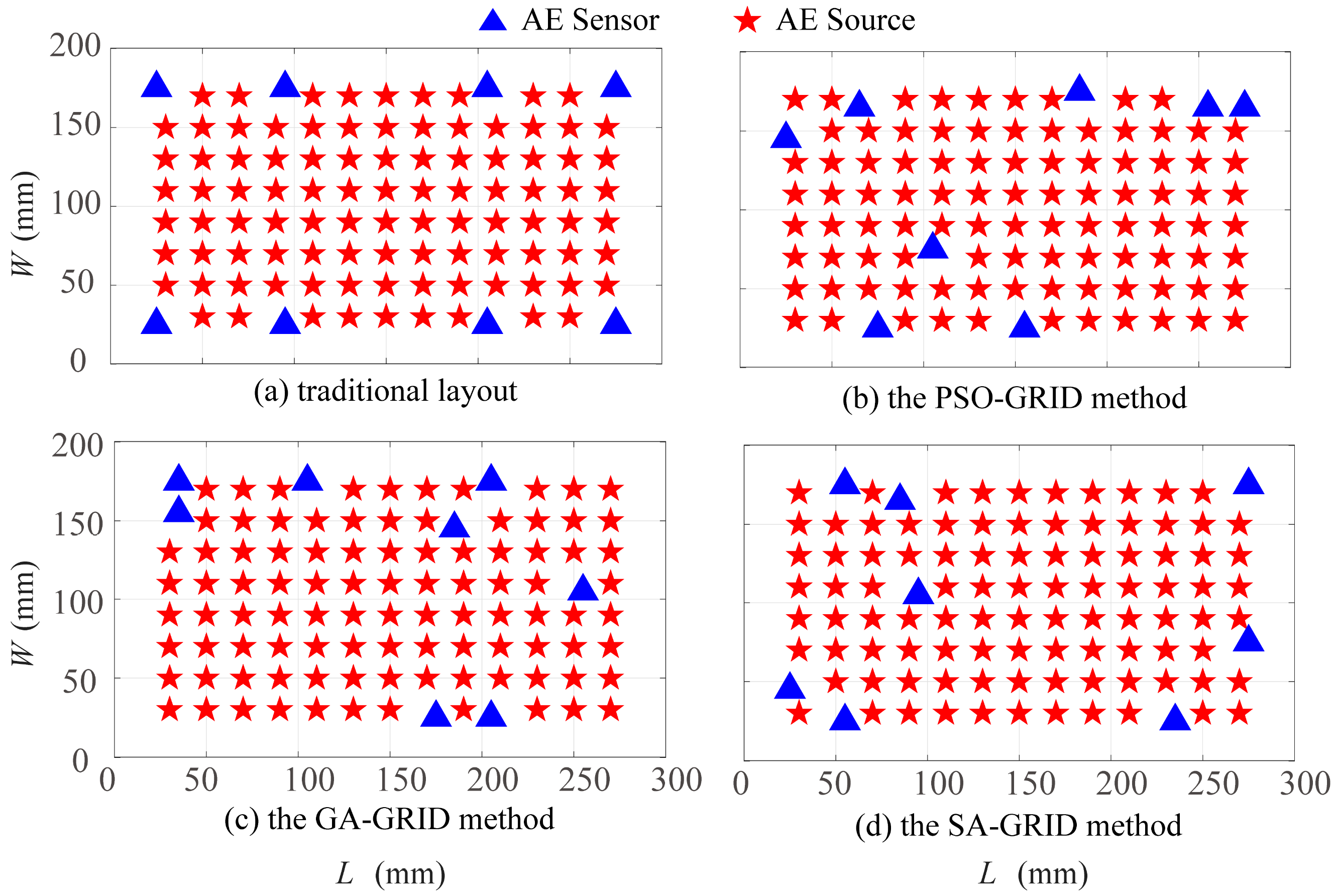
Based on this setup, a synthetic tests on sensor layout optimization were conducted. Eight sensors were used in this test. Traditional sensor layouts are often regular and symmetric. Therefore, to simulate traditional layouts, the traditional layout was designed with regular symmetry. In order to conduct comparative experiments with the PSO, we also recorded the sensor layout optimization results obtained using the GA and SA for source location. The methods combining PSO, GA, and SA with the grid search method were defined as the PSO-GRID method, GA-GRID method, and SA-GRID method, respectively. The sensor distributions obtained by different methods under the same initial layout are shown in Figure 4 and Table 1. Compared to the traditional layout, the sensor distributions optimized by these three methods tend to concentrate along the boundaries of the monitoring area, while maintaining some sensors in the central region.
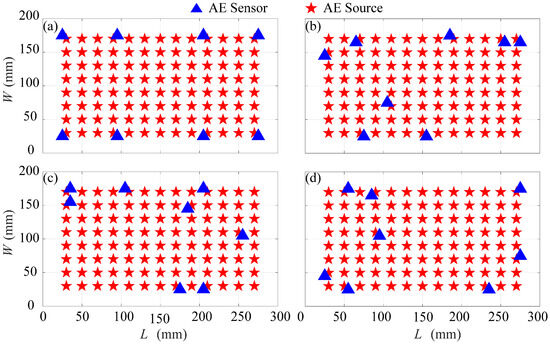
Figure 4.
Sensor layouts before and after optimization. (a) Traditional sensor layout. (b–d) Sensor layout after optimization using the PSO-GRID method, GA-GRID method, and SA-GRID method.

Table 1.
Sensor layout coordinates under random layout without optimization and different optimization algorithms.
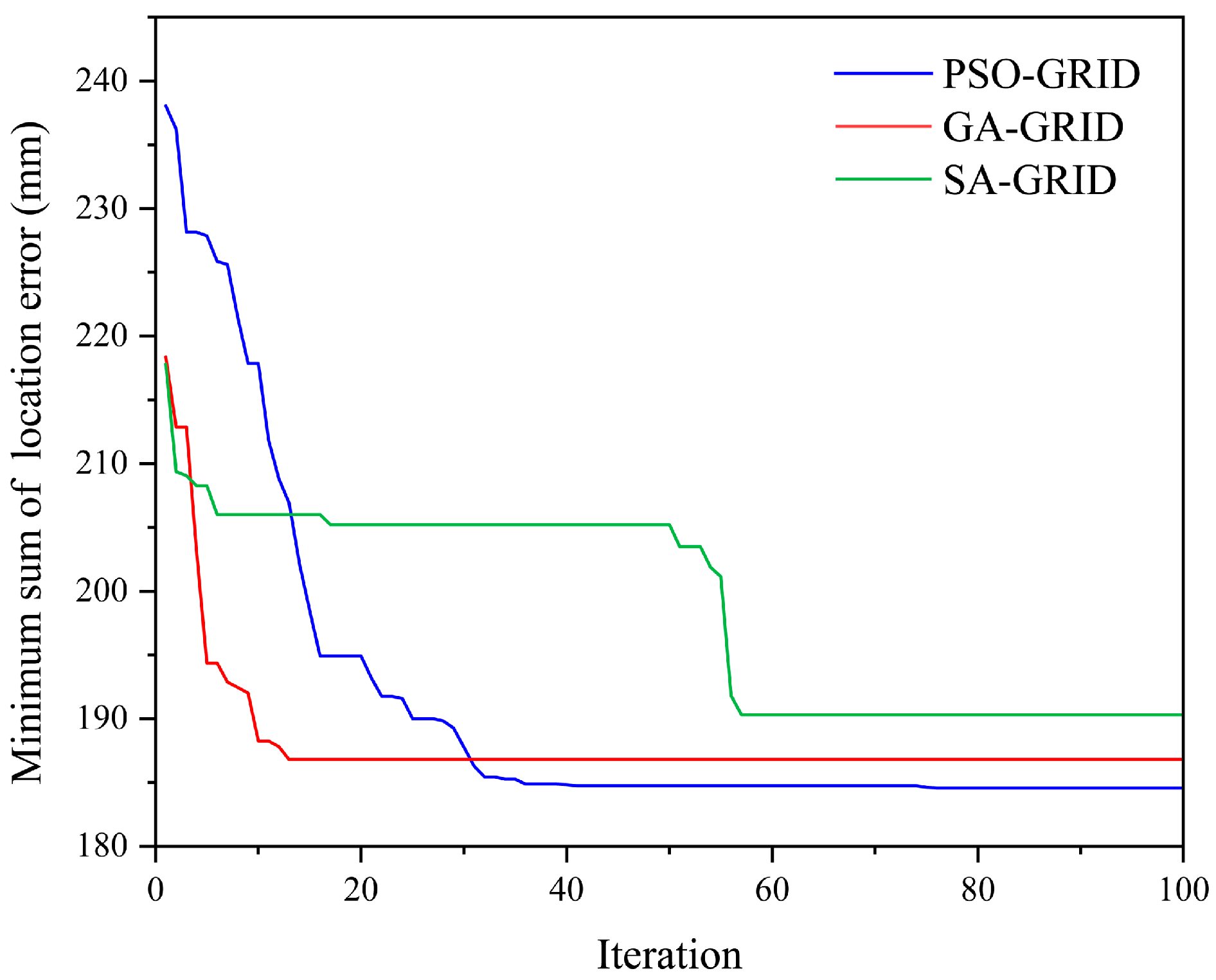
During the optimization process, the global error sums of these three models (Figure 5) were recorded to evaluate their performance in sensor layout optimization. The GA-GRID method demonstrates rapid convergence in the early stage, achieving a low error value more quickly. Although the PSO-GRID method has a slightly slower convergence than the GA-GRID method, it achieves a slightly lower final error value than the GA-GRID method. In contrast, the SA-GRID method has a slower convergence rate and a higher final location error. The result indicates that the performance of the SA-GRID method is not as effective as the other two algorithms.
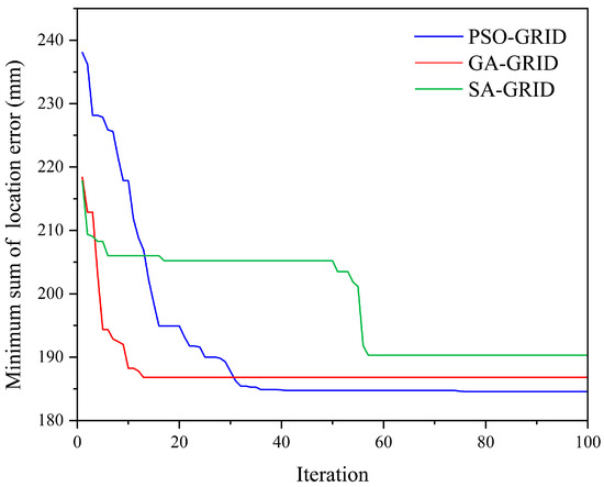
Figure 5.
Global minimum error convergence for the PSO-GRID method, GA-GRID method, and SA-GRID method.
3.2. Location Results
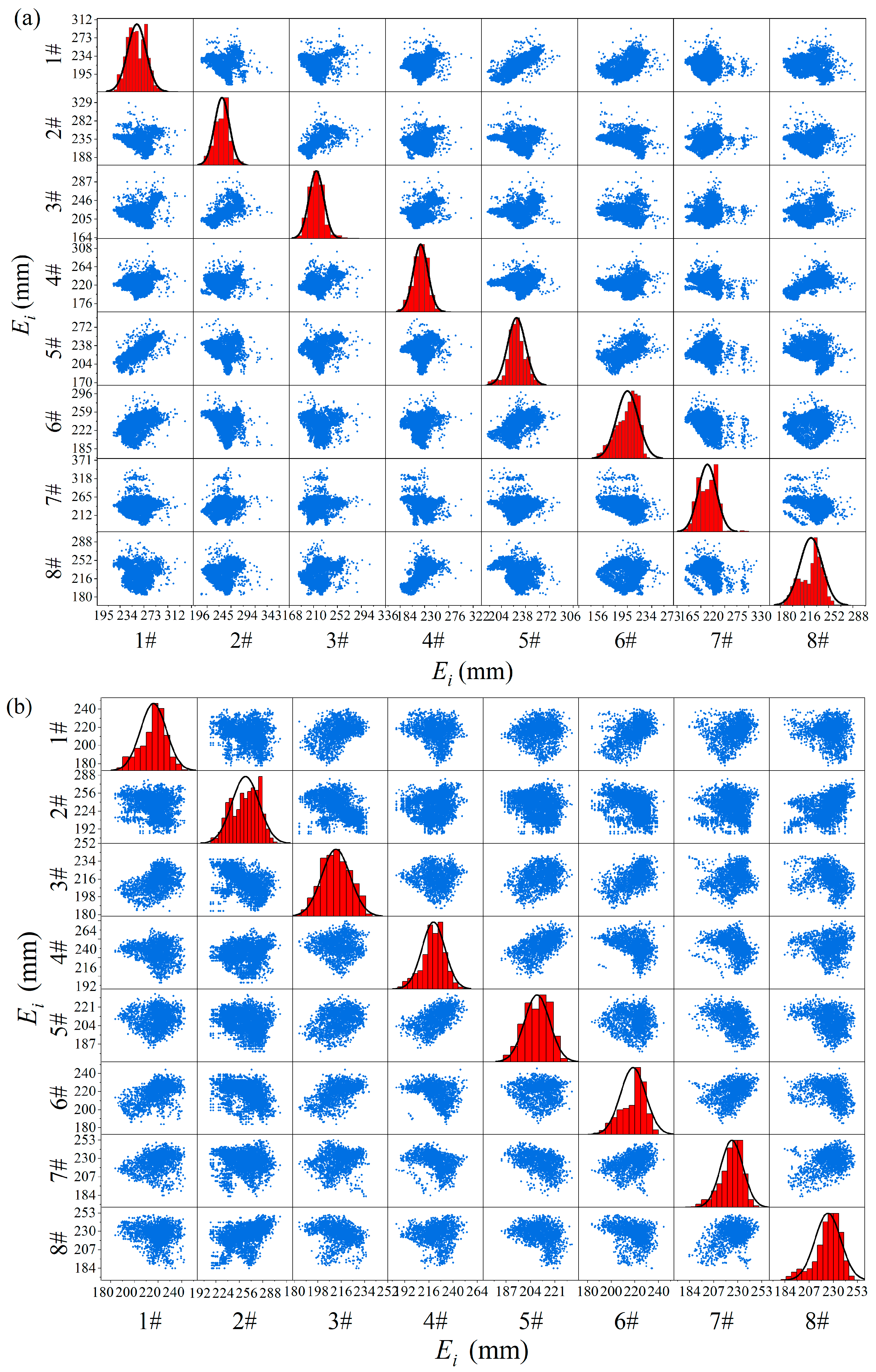
To analyze the performance of different optimization algorithms during the sensor layout optimization process, we recorded the location error values of all sensors under different layouts at each iteration (Figure 6). The diagonal elements of the matrix scatter plots show the distribution histograms of individual sensors during the optimization process, while the off-diagonal elements display the scatter plots of error values between different sensors.
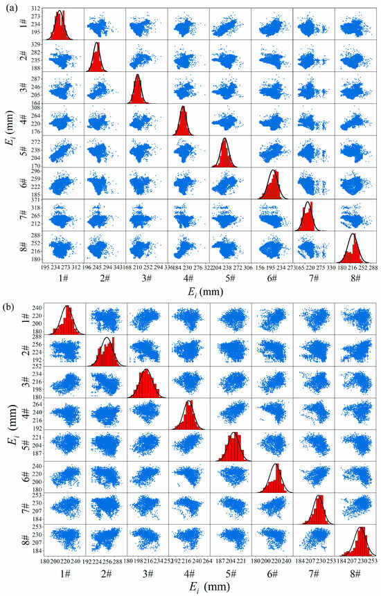
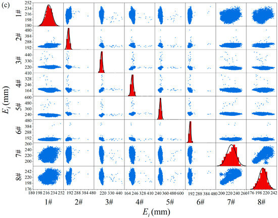
Figure 6.
Scatter plots of the Ei matrix of each sensor under different optimization algorithms. (a) PSO-GRID method. (b) GA-GRID method. (c) SA-GRID method. The # indicates the number of each sensor. The blue dot represents the location error data point of a sensor under specific conditions. The reference bar is a histogram showing the error distribution of the sensor. The black line represents the fitting curve of the sensor error.
By comparing these three methods, it is evident that the error distribution in the matrix scatter plot of the PSO-GRID method is more dispersed than that of GA and SA. This dispersed distribution indicates that PSO can achieve global optimal search, effectively control the error range, and make the results more reliable. In contrast, the GA-GRID method’s scatter plot shows a more scattered and irregular distribution. While GA has strong global exploration capabilities, the convergence is less stable and results in greater randomness in errors. The SA-GRID method exhibits high density in local regions, which indicates that errors are concentrated within a limited range. However, the local density does not indicate strong overall optimization performance, suggesting that SA is susceptible to local optima. SA lacks global consistency, leading to error concentration on a limited number of sensors, and its optimization performance is inferior to the global search capability and stability of PSO. In summary, the PSO-GRID method combines the advantages of global exploration and rapid convergence. The optimization results demonstrate stability and consistency, showing significantly better performance compared to the instability and dispersion of GA and the local concentration of SA.
Furthermore, the width of the red bars in the diagonal elements of the Figure 6 reflect the spread of the error distribution for each sensor. A wider distribution (e.g., Figure 6b) indicates that the algorithm explores a broader range of solutions. However, the irregular and scattered nature of the GA-GRID’s distribution suggests instability and randomness in its optimization process, which can lead to less reliable results. In contrast, the moderately wide and consistent distribution observed in the PSO-GRID (Figure 6a) demonstrates a balance between global exploration and stable convergence. This allows PSO to effectively search the solution space while maintaining robustness and avoiding local optima. On the other hand, the narrow distribution in the SA-GRID (Figure 6c) reflects high local consistency but highlights its susceptibility to local optima, limiting its global search capability. Overall, the PSO-GRID achieves the best trade-off between exploration and stability, making it the most effective method for sensor layout optimization.
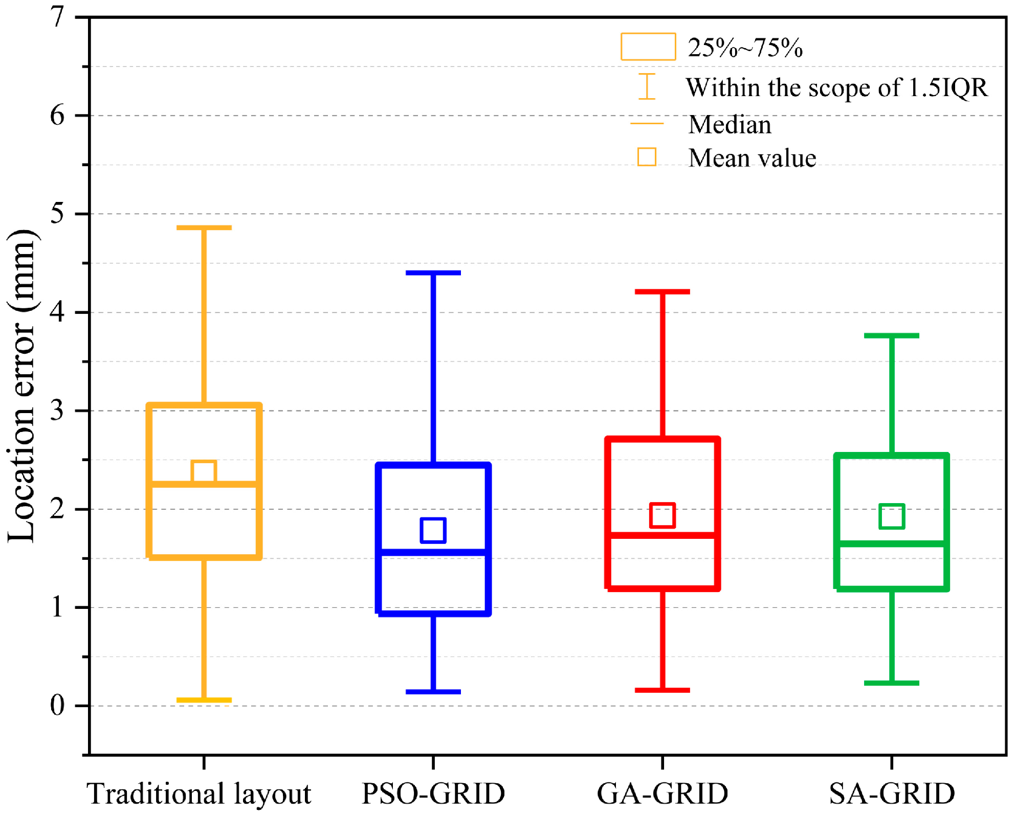
The accuracy of the AE event location is a critical indicator to evaluate sensor layout effectiveness. The location errors are shown in Figure 7. The traditional layout has a relatively high average location error of 2.37 mm. After optimization using the PSO-GRID method, GA-GRID method, and SA-GRID method, the location errors decreased to 1.78 mm, 1.93 mm, and 1.92 mm. Compared with the traditional layout, the GA-GRID method, and the SA-GRID method, the PSO method improved location accuracy by 24.89%, 7.81%, and 7.39%, respectively. The results indicate that the PSO-GRID method achieves the best performance in reducing location errors, with the most significant improvement.

Figure 7.
Box plot of location errors for traditional and different optimization algorithm layouts.
3.3. Noise Resistance Testing of the Synthetic Model
In practical applications, sensors are inevitably influenced by noise, necessitating an evaluation of the proposed optimization method’s adaptability to various noise environments. Gaussian noises with standard deviations of 0.5 μs, 2 μs, and 5 μs was applied to the theoretical P-wave travel time data. The location results are shown in Figure 8, where it is evident that the PSO-GRID method was the best performer, achieving location accuracy improvements of 24.89% (0.5 μs), 12.59% (2 μs), and 15.06% (5 μs) under the three noise conditions. A comparison of the location accuracy between PSO-GRID and the other two models is shown in Figure 8. This result confirms that PSO is better suited to handle high-noise data and provides a robust solution.
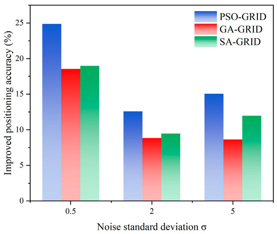
Figure 8.
Changes in location accuracy under different noise parameters.
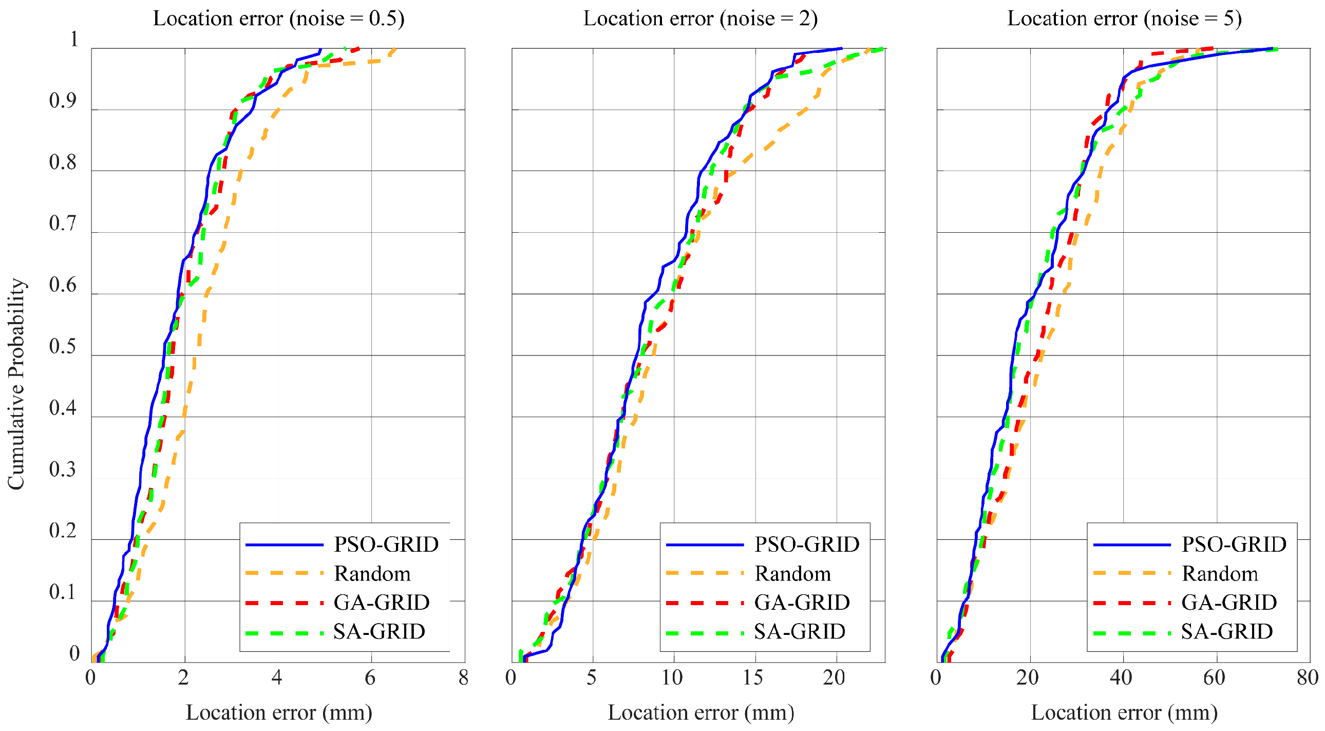
Additionally, Figure 9 generated a cumulative distribution function (CDF) plot based on location error. The PSO-GRID method optimization algorithm consistently delivers the best location accuracy improvement across all noise levels. Under low-noise conditions (σ = 0.5 μs), the cumulative probability curve for PSO is closer to the lower error range compared to the GA-GRID method and the SA-GRID method. This indicates higher location accuracy and stability. As noise increases to medium and high levels (σ = 2 μs and σ = 5 μs), the PSO-GRID method still maintains strong noise resistance and shows significant performance gap compared to the traditional layout. In contrast, the GA-GRID method and SA-GRID method gradually approach the performance of traditional layouts and become more sensitive to noise. Overall, the PSO-GRID method demonstrates the best location performance under various noise conditions. It is the preferred method for optimizing sensor layouts.
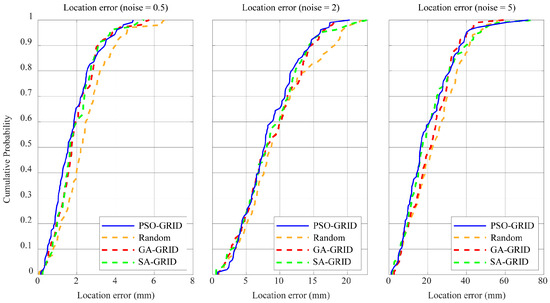
Figure 9.
Cumulative distribution function of location error under different noise standard deviations.
4. Experimental Test
4.1. Experimental Setup
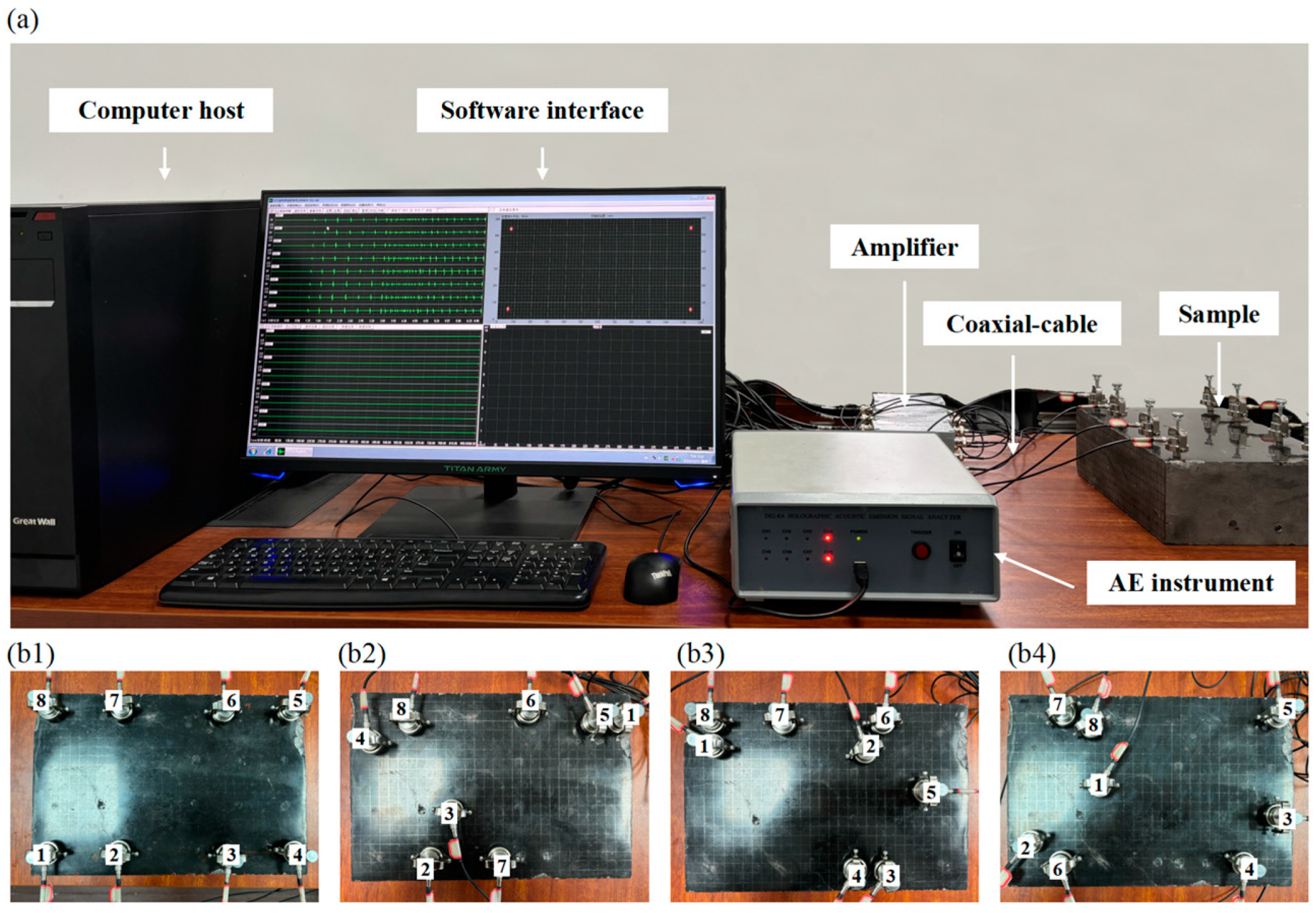
To further verify the effectiveness of the proposed method, this study conducted a laboratory AE PLB experiment on the traditional layout and layouts optimized by the PSO-GRID method, GA-GRID method, and SA-GRID method. The DS2 AE equipment is made by the Softland Times company in Beijing, China (Figure 10). The dimensions of the granite sample and the P-wave velocity are consistent with the simulation test, as listed in Table 1 in Section 3.1. The planar distribution of AE sources and sensors is shown in Figure 11. The sample size is 300 mm × 200 mm, and the surface is divided into 10 mm × 10 mm grid cells, with PLB performed at grid nodes to simulate AE sources. Due to operational constraints, some grid points near the sensors will not conduct PLB experiments.

Figure 10.
Detailed diagram of AE monitoring system and layouts. (a) AE equipment and sample. (b1) Traditional layout. (b2) PSO-GRID method layout. (b3) GA-GRID method layout. (b4) SA-GRID method layout. The numbers in (b1–b4) represent the sensor ID.
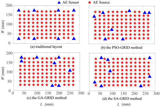
Figure 11.
Distribution of AE sources and sensor locations.
In this experiment, eight sensors were configured to capture signals emitted from the AE sources, all amplified by preamplifiers. The amplifier was fixed to 40 dB and the amplified signals were recorded by the DS5-8A device, with a sampling frequency set to 3 MHz. The equipment is made by the Softland Times company in Beijing, China. A total of 96 AE source points were used to collect signals for the optimized layouts of the traditional method, PSO-GRID method, GA-GRID method, and SA-GRID method. Each method utilized the same number of source points to ensure consistency in the comparison.
4.2. Experimental Data Processing
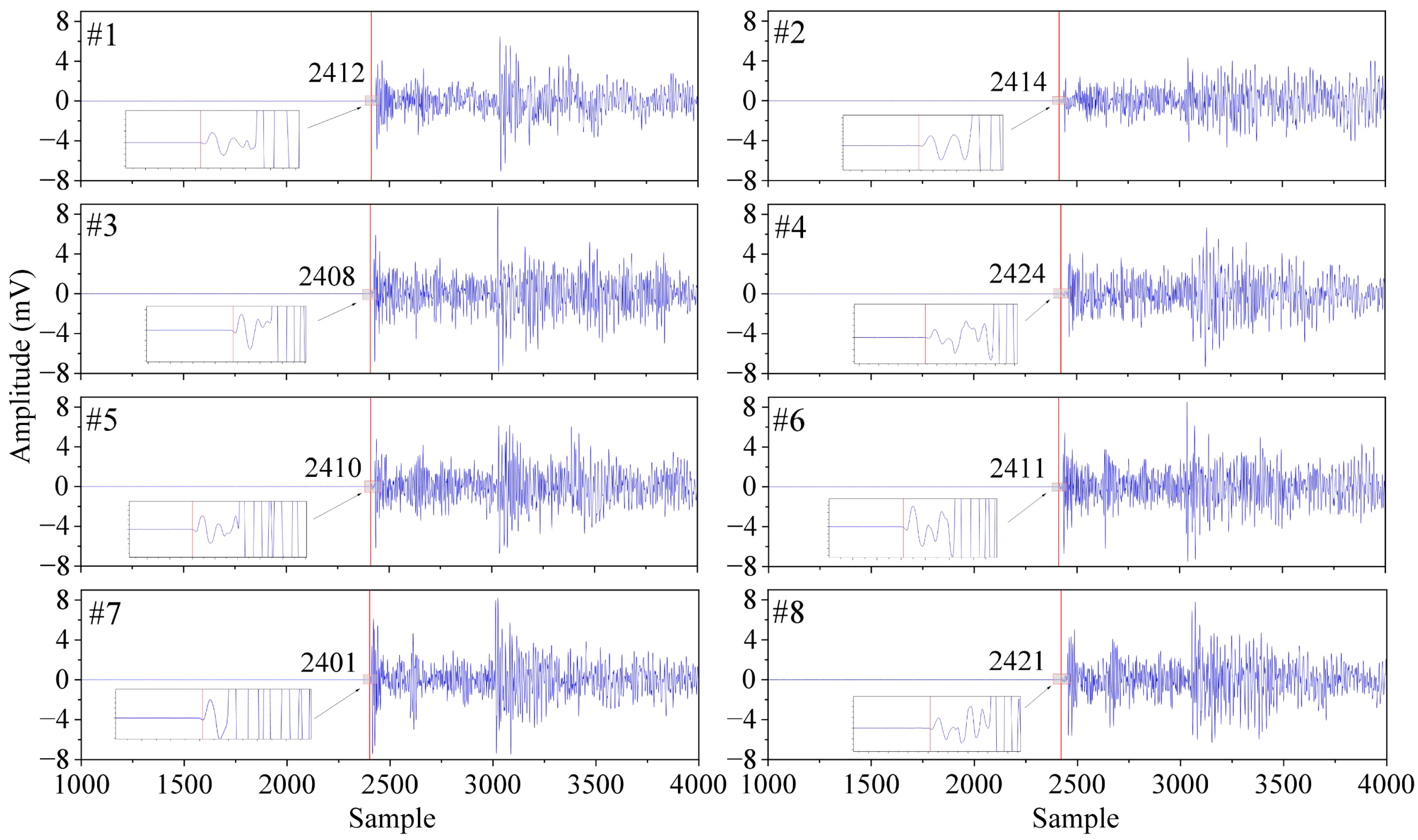
After the monitoring signals were received, they were analyzed using MATLAB (R2024a) software. The waveform of the AE signals received by the sensors is shown in Figure 12, with the P-wave first arrival data obtained using the AIC automatic picking method [24]. The use of the AIC method to pick P-wave arrivals is easily affected by trailing waves, which causes data instability. To address this issue, this study employed manual calibration and removed the origin time to ensure the accuracy of arrival time picking and subsequent location verification.
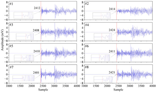
Figure 12.
Waveform of PLB events and P-wave first arrival picking results. The red solid line indicates the picked P-wave arrival time. The blue line represents the amplitude change of the acoustic emission signal recorded by each sensor. The number in the top left corner represents the sensor ID.
4.3. Location Test
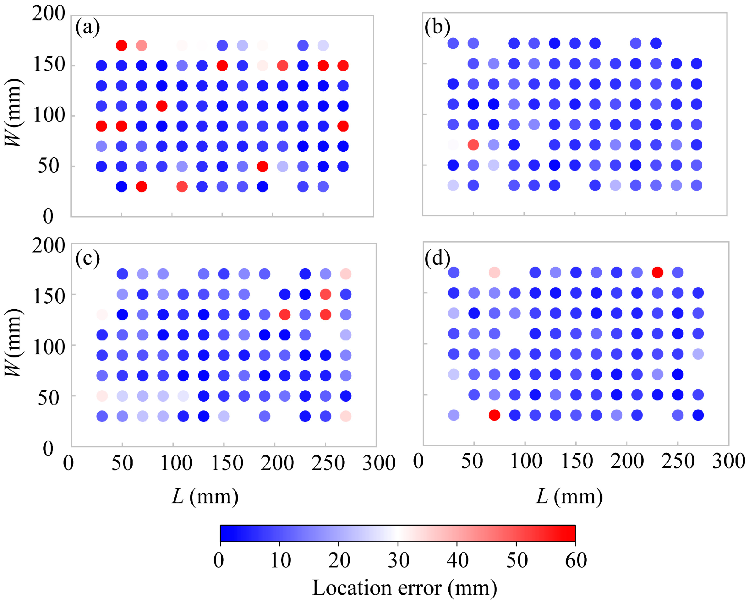
The layouts obtained from the synthetic tests in Section 3 were used in a location experiment, with the PLB points and AE location results shown in Figure 13b. The PSO-GRID method achieved the best performance in location accuracy. The error between the location result and actual location was generally small. The overall distribution of location errors was more uniform and the location accuracy significantly improved. In contrast, the GA-GRID method (Figure 13c) and SA-GRID method (Figure 13d) performed better than the traditional layout (Figure 13a). However, their location errors increased significantly in certain regions. This shows that GA and SA are more susceptible to traditional values.
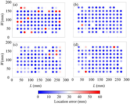
Figure 13.
Location results of AE experiments under different layouts. (a) Traditional. (b) PSO-GRID. (c) GA-GRID. (d) SA-GRID.
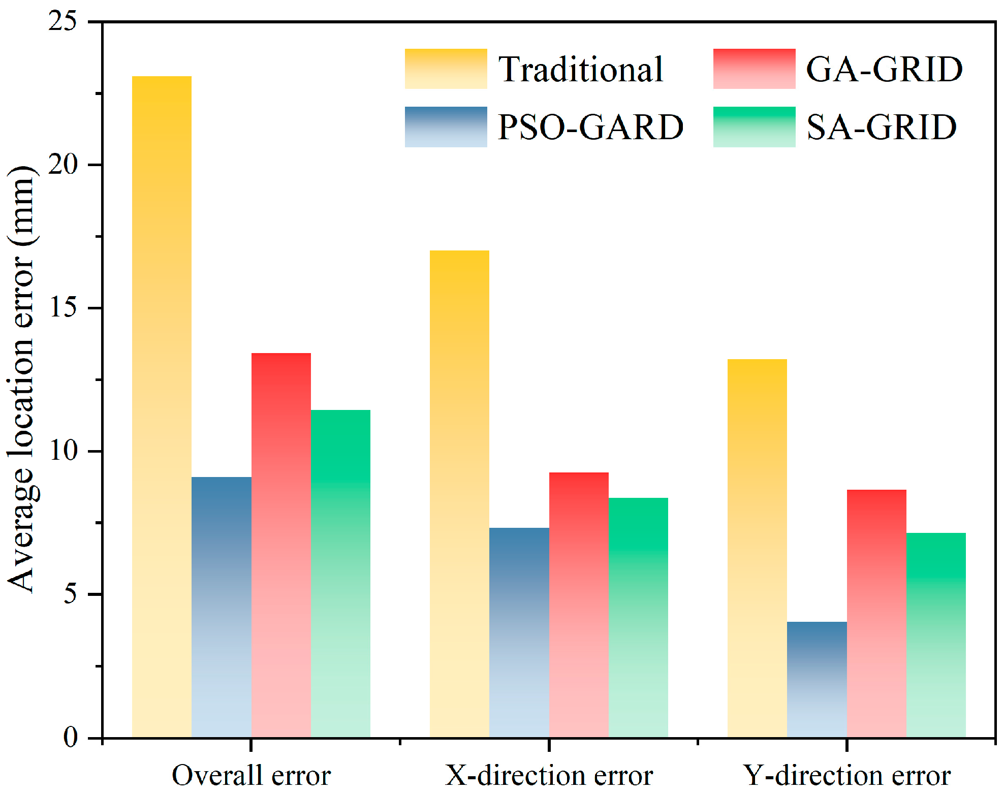
The average location errors before and after optimization are shown in Figure 14. The average location error for the traditional layout was 22.94 mm, while the PSO-GRID method, GA-GRID method, and SA-GRID method optimized layouts achieved average location errors of 9.37 mm, 13.73 mm, and 11.78 mm. The proposed optimization method improved location accuracy by 59.15%, 31.76%, and 20.46% compared to the traditional layout, GA-GRID method, and SA-GRID method, respectively. This demonstrates the superior performance of the proposed method in enhancing location accuracy.
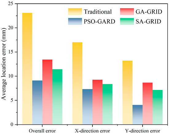
Figure 14.
Overall average location error and average location error in X and Y directions under different sensor layouts.
The PSO-GRID method demonstrated significant advantages in overall errors, X-direction errors, and Y-direction errors. Compared with the traditional layout, the PSO-GRID method achieved a substantial reduction in error. This shows that it has the most notable optimization results. In comparison with the GA-GRID method and SA-GRID methods, the PSO-GRID method exhibited lower errors. In summary, the PSO-GRID method layout demonstrates significant advantages in accuracy and stability during the PLB experiment.
5. Discussions
5.1. Influence of Sensor Layouts
The determination of an optimal sensor layout is essential to ensure the smooth implementation of subsequent monitoring tasks in AE monitoring. Based on traditional empirical understanding, this study initially established a regular and partially enclosed sensor layout. However, through the optimization process, the sensor layout gradually evolved into a pattern where some sensors were distributed along the boundaries of the monitoring area, while others were located in the central region. Gomes [25] used a multi-objective optimization method to optimize the sensor layout. This approach focused on the maximization of the Fisher information matrix and the improvement of pattern reconstruction accuracy. The resulting layout was similar to the findings of this study.
This layout mainly results from a natural formation due to the optimization requirements of the objective function. To minimize the error between the predicted travel time and the actual travel time, the sensors must cover all potential seismic source points within the monitored area. Although arranging sensors solely along the boundaries can better envelop the monitored area, it will lead to increased errors in the distant central region. During the optimization process, the algorithm drives a small number of sensors to move from the boundaries toward the center to reduce errors in the central region. The combined effect of central and boundary sensors ensures a balance between global coverage and local accuracy, ultimately reducing the overall location errors.
5.2. Influence of Optimization Algorithms
Sensor layout optimization is heavily influenced by the solution of the objective function. Selecting an appropriate algorithm to solve the objective function is key to the optimization process. PSO utilizes particle collaboration to achieve global exploration and prevent falling into local optima. Sadeq [26] applied PSO integrated with a triple-structure encoding method to optimize sensor placement in structural health monitoring. In sensor layout optimization, sensor locations are treated as continuous variables. GA’s crossover and mutation operations may introduce redundancy, reducing search efficiency, where PSO does not have this issue and is more suitable for sensor layout optimization. Additionally, GA requires solutions to be encoded into discrete or binary forms, which can lead to decreased precision. In terms of computational efficiency, PSO is also more suitable for sensor layout optimization because its update equations are simple and the computational complexity is low. Additionally, the independent particle characteristics of the algorithm make it convenient for parallel processing. In contrast, the complex population operations of GA and the slow cooling process of SA make them difficult to achieve the efficiency required for engineering applications.
To further evaluate the performance of these three algorithms in AE location, we provide two types of analyses (Figure 15). The first is the fitness variation curves with iterations that show confidence intervals. The second is the total time distribution in bar charts for each algorithm. Figure 15a shows that all these three algorithms eventually converged to similar fitness levels. The GA exhibited larger fluctuations during convergence, which is due to the randomness of its genetic operations. In contrast, PSO and SA demonstrated greater stability, with SA exhibiting relatively low fitness values from the outset, attributed to its acceptance criteria. Figure 15b reveals that PSO had the shortest runtime, mostly concentrated between 0 and 1 s, while GA’s runtime was more dispersed, mainly focused between 1 and 3 s. Although SA is more stable, its runtime was significantly longer, mainly concentrated between 6 and 8 s. The comprehensive analysis indicates that SA has advantages in stability but demonstrates low computational efficiency. In contrast, PSO achieved a good balance between efficiency and performance.
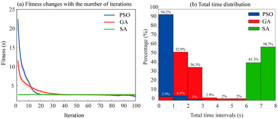
Figure 15.
Comparison of fitness variation and time distribution. The light-colored area represents the 95% confidence interval of the fitness value.
5.3. Influence of the Number of Sensors
In the location study of AE events, the number of sensors has a significant impact on the location errors. Generally, as the number of sensors increases, the location error will gradually decrease, thereby improving the location accuracy. Chen et al. [27] conducted an experimental study on the effect of the number of sensors on the location accuracy of AE events. The experimental results show that as the number of sensors involved in the location calculation increases, the maximum and average location errors both show a trend of gradually decreasing, and the location accuracy improves accordingly. However, there is an optimal value for the number of sensors. When the number of sensors reaches this optimal value, the location accuracy reaches the optimal value. Further increasing the number of sensors will increase the minimum location errors.
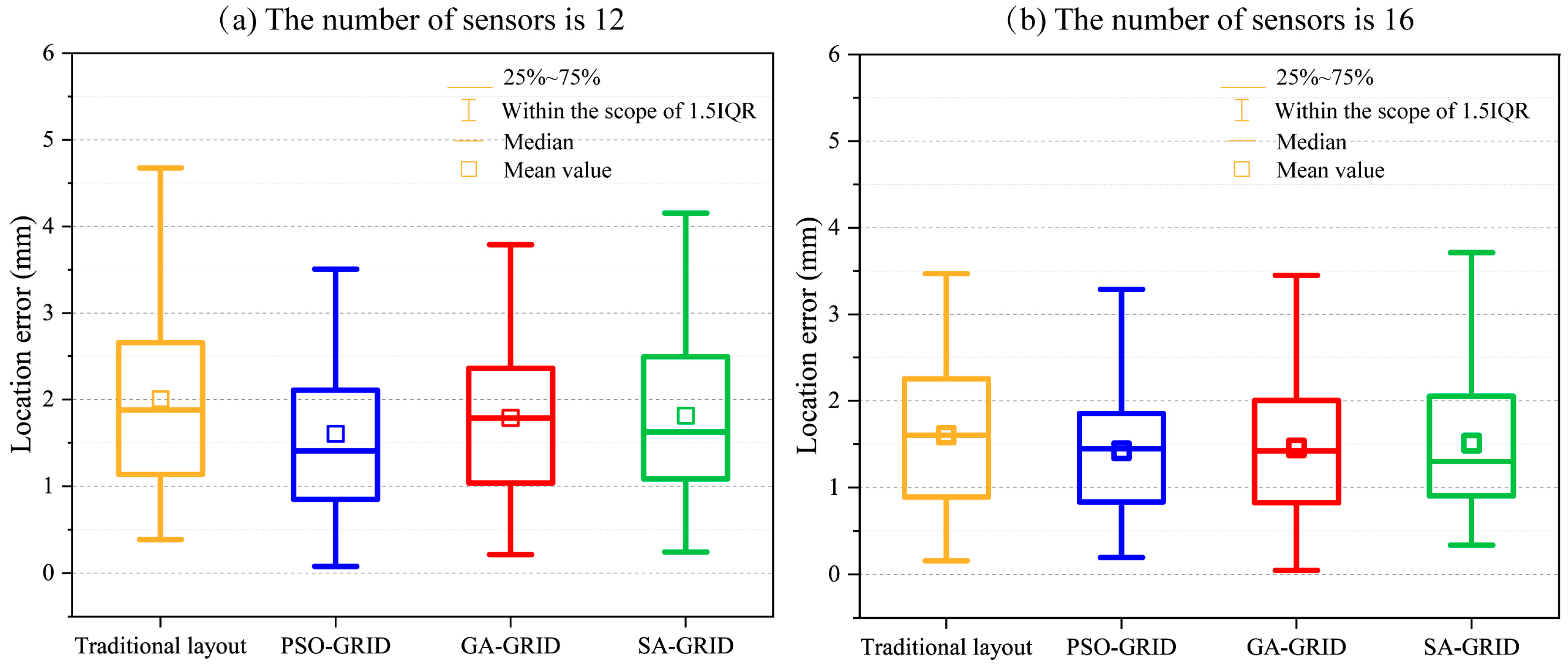
To deeply explore the impact of the number of sensors on the location accuracy of AE sources, this study increases the number of sensors to 12 and 16 respectively (Figure 16), while keeping other parameters consistent with Section 3. The initial layout still uses the traditional layout with certain rules. The experimental results (Table 2) show that as the number of sensors increases, the overall average location errors shows a decreasing trend, but the decrease is not significant. Further comparison of the location effects of different methods shows that when the number of sensors increases, compared with the GA-GRID method and SA-GRID method, the PSO-GRID method can still maintain a lower average location error value. This indicates that as the number of sensors increases, the method proposed in this study still has a significant advantage in improving location accuracy.
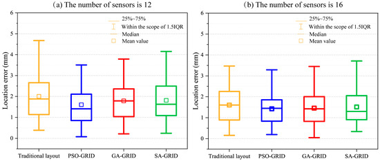
Figure 16.
Effect of sensor number to source location results.
Table 2.
Average positioning error of different sensor numbers.
In general, increasing the number of sensors can improve location accuracy to a certain extent. This is because more sensors can capture richer signal information, which provides more favorable data support for the precise location of AE sources. However, considering factors such as computational efficiency and cost in practical engineering applications, the model constructed in this study is mainly aimed at the monitoring of rock crack development and other fields. In such application scenarios, the location accuracy provided by eight sensors can already meet the actual requirements.
Overall, the optimization of sensor layout is influenced by multiple factors, and even after optimization, location errors may still exhibit uncertainty. This is primarily due to factors such as the possibility of achieving a locally optimal layout, although the optimized layout in this study demonstrates better performance compared to other layouts. Additionally, experimental data can also affect the location results, ultimately contributing to the uncertainty in the source location.
6. Conclusions
To address the issues of traditional sensor optimization methods being difficult to understand and inefficient, a minimum travel time difference optimization method based on the PSO and grid search method is proposed. The method is compared with the GA-GRID method and SA-GRID method to verify the superiority of the proposed method. Finally, the feasibility and effectiveness of the method were verified through laboratory AE experiments. The main conclusions and findings are as follows:
- A sensor network layout optimization method based on the minimum travel-time difference is developed by combining the PSO method with the grid search methods. The method establishes a location objective function based on source travel-time theory and optimizes the function by PSO. It integrates grid search to systematically examine potential sensor locations, thereby determining the optimal sensor layout. This approach focuses on optimizing source location and is easy to understand.
- The optimization method proposed in this study demonstrated excellent location accuracy and strong noise resistance in synthetic tests. In the synthetic test, the PSO-GRID method, GA-GRID method, and SA-GRID method, improving location accuracy by 24.89%, 7.81%, and 7.39%, respectively. Furthermore, under varying noise levels the PSO-GRID method maintained high location accuracy, achieving improvements of 24.89%, 12.59%, and 15.06% across three noise conditions. These results validate the effectiveness and robustness of the proposed method in synthetic scenarios.
- The proposed optimization method performed well in laboratory AE experiments. In AE experiments, the PSO-GRID method improved location accuracy by 59.15%, 31.76%, and 20.46% compared to the traditional layout, GA-GRID method, and SA-GRID method, respectively. It also demonstrated high computational efficiency, minimal error fluctuations, and optimal performance under various noise conditions, requiring minimal parameter adjustment. These results confirm PSO-GRID as the most reliable and practical choice for location optimization.
Author Contributions
Methodology, validation, analysis, data curation, writing—original draft preparation, Y.C.; conceptualization and Writing—review, X.S.; conceptualization, supervision, validation, and writing—review and editing, L.L.; resources, data curation, Y.R., X.L., Y.Z., X.W., Z.L., Y.T., Y.P. and G.X. All authors have read and agreed to the published version of the manuscript.
Funding
This research was funded by State Key Laboratory of Strata Intelligent Control and Green Mining Co-founded by Shandong Province and the Ministry of Science and Technology, Shandong University of Science and Technology (no. SICGM2023301).
Data Availability Statement
Research data are available on request.
Acknowledgments
The authors thank the State Key Laboratory of Coal Mine Disaster Dynamics and Control, Chongqing University, for their assistance.
Conflicts of Interest
Authors Xiaoying Li, Zhuqing Li and Guanghua Xiang were employed by the Beijing 5lWORLD Digital Twin Technology Co., Ltd. Yu Zhang was employed by the Y-Link (Wuhan) Technology Co., Ltd. Xiao Wu was employed by the Chongqing Top-Tech Information Co., Ltd. The remaining authors declare that the research was conducted in the absence of any commercial or financial relationships that could be construed as potential conflicts of interest.
References
- Lockner, D. The Role of Acoustic-Emission in the Study of Rock Fracture. Int. J. Rock Mech. Min. Sci. 1993, 30, 883–899. [Google Scholar] [CrossRef]
- Recoquillay, A.; Pénicaud, M.; Serey, V.; Lefeuve, C. Source Reconstruction for Acoustic Emission Signals Clustering and Events Nature Identification. Application to a Composite Pipe Bending Test. Mech. Syst. Signal Process. 2025, 224, 111954. [Google Scholar] [CrossRef]
- Huang, L.Q.; Wu, X.; Li, X.B.; Wang, S.F. Influence of Sensor Array on Ms/Ae Source Location Accuracy in Rock Mass. Trans. Nonferrous Met. Soc. China 2023, 33, 254–274. [Google Scholar] [CrossRef]
- Kijko, A. Algorithm for Optimum Distribution of a Regional Seismic Network—I. Pure Appl. Geophys. 1977, 115, 999–1009. [Google Scholar] [CrossRef]
- Kijko, A. Algorithm for Optimum Distribution of a Regional Seismic Network—II. Analysis of Accuracy of Location of Local Earthquakes Depending on Number of Seismic Stations. Pure Appl. Geophys. 1977, 115, 1011–1021. [Google Scholar] [CrossRef]
- Rabinowitz, N.; Steinberg, D.M. Optimal Configuration of a Seismographic Network—A Statistical Approach. Bull. Seismol. Soc. Am. 1990, 80, 187–196. [Google Scholar] [CrossRef]
- Jones, R.H.; Rayne, C.M.; Ulf, L. The Use of a Genetic Algorithm for the Optimal Design of Microseismic Monitoring Networks. In Proceedings of the Rock Mechanics in Petroleum Engineering, Delft, The Netherlands, 29–31 August 1994. [Google Scholar]
- Kraft, T.; Mignan, A.; Giardini, D. Optimization of a Large-Scale Microseismic Monitoring Network in Northern Switzerland. Geophys. J. Int. 2013, 195, 474–490. [Google Scholar] [CrossRef]
- Rosa-Cintas, S.; Galiana-Merino, J.J.; Alfaro, P.; Rosa-Herranz, J. Optimizing the Number of Stations in Arrays Measurements: Experimental Outcomes for Different Array Geometries and the F-K Method. J. Appl. Geophys. 2014, 102, 96–133. [Google Scholar] [CrossRef]
- De Landro, G.; Picozzi, M.; Russo, G.; Adinolfi, G.M.; Zollo, A. Seismic Networks Layout Optimization for a High-Resolution Monitoring of Induced Micro-Seismicity. J. Seismol. 2020, 24, 953–966. [Google Scholar] [CrossRef]
- Zhou, Z.L.; Zhao, C.C.; Huang, Y.H. An Optimization Method for the Station Layout of a Microseismic Monitoring System in Underground Mine Engineering. Sensors 2022, 22, 4775. [Google Scholar] [CrossRef] [PubMed]
- Li, N.; Ge, M.C.; Wang, E.Y.; Zhang, S.H. The Influence Mechanism and Optimization of the Sensor Network on the Ms/Ae Source Location. Shock Vib. 2020, 2020, 2651214. [Google Scholar] [CrossRef]
- Li, G.; Chen, J.; Han, M.; Gajraj, A.; Xing, Y.; Wu, F.; Liu, H.; Yin, C. Accurate Microseismic Event Location Inversion Using a Gradient-Based Method. In Proceedings of the SPE Annual Technical Conference and Exhibition, San Antonio, TX, USA, 8–10 October 2012. [Google Scholar]
- Thurber, C.H. Nonlinear Earthquake Location—Theory and Examples. Bull. Seismol. Soc. Am. 1985, 75, 779–790. [Google Scholar] [CrossRef]
- Holland, J.H. Genetic Algorithms. Sci. Am. 1992, 267, 66–73. [Google Scholar] [CrossRef]
- Kennedy, J.; Eberhart, R. Particle Swarm Optimization. In Proceedings of the ICNN’95-International Conference on Neural Networks, Perth, WA, Australia, 27 November–1 December 1995; pp. 1942–1948. [Google Scholar]
- Basu, A.; Frazer, L.N. Rapid Determination of the Critical Temperature in Simulated Annealing Inversion. Science 1990, 249, 1409–1412. [Google Scholar] [CrossRef] [PubMed]
- Dhiman, G.; Kumar, V. Spotted Hyena Optimizer: A Novel Bio-Inspired Based Metaheuristic Technique for Engineering Applications. Adv. Eng. Softw. 2017, 114, 48–70. [Google Scholar] [CrossRef]
- Pace, F.; Santilano, A.; Godio, A. A Review of Geophysical Modeling Based on Particle Swarm Optimization. Surv. Geophys. 2021, 42, 505–549. [Google Scholar] [CrossRef] [PubMed]
- Chen, B.; Feng, X.; Li, S.; Yuan, J.; Xu, S. Microseism Source Location with Hierarchical Strategy Based on Particle Swarm Optimization. Chin. J. Rock Mech. Eng. 2009, 28, 740–749. [Google Scholar]
- Raorane, S.; Ercan, T.; Papadimitriou, C.; Packo, P.; Uhl, T. Bayesian Optimal Sensor Placement for Acoustic Emission Source Localization with Clusters of Sensors in Isotropic Plates. Mech. Syst. Signal Process. 2024, 214, 111342. [Google Scholar] [CrossRef]
- Dong, L.J.; Cao, H.; Hu, Q.C.; Zhang, S.; Zhang, X.H. Error Distribution and Influencing Factors of Acoustic Emission Source Location for Sensor Rectangular Network. Measurement 2024, 225, 113983. [Google Scholar] [CrossRef]
- Rui, Y.C.; Zhu, C.J.; Chen, J.; Zhou, Z.L.; Pu, Y.Y. Study on Sensor Network Optimization for Ms/Ae Monitoring System Using Fisher Information and Improved Encoding Framework. IEEE Sens. J. 2024, 24, 22958–22973. [Google Scholar] [CrossRef]
- Sleeman, R.; van Eck, T. Robust Automatic P-Phase Picking: An on-Line Implementation in the Analysis of Broadband Seismogram Recordings. Phys. Earth Planet. Inter. 1999, 113, 265–275. [Google Scholar] [CrossRef]
- Gomes, G.F.; De Almeida, F.A.; Lopes Alexandrino, P.D.S.; Da Cunha, S.S., Jr.; De Sousa, B.S.; Ancelotti, A.C., Jr. A Multiobjective Sensor Placement Optimization for Shm Systems Considering Fisher Information Matrix and Mode Shape Interpolation. Eng. Comput. 2019, 35, 519–535. [Google Scholar] [CrossRef]
- Kord, S.; Taghikhany, T.; Madadi, A.; Hosseinbor, O. A Novel Triple-Structure Coding to Use Evolutionary Algorithms for Optimal Sensor Placement Integrated with Modal Identification. Struct. Multidiscip. Optim. 2024, 67, 58. [Google Scholar] [CrossRef]
- Chen, Y.L.; Zhang, M.W.; Wu, H.S.; Zhang, K.; Qian, D.Y. Improving the Positioning Accuracy of Acoustic Emission Events by Optimizing the Sensor Deployment and First Arrival Signal Picking. IEEE Access 2020, 8, 71160–71172. [Google Scholar] [CrossRef]


Disclaimer/Publisher’s Note: The statements, opinions and data contained in all publications are solely those of the individual author(s) and contributor(s) and not of MDPI and/or the editor(s). MDPI and/or the editor(s) disclaim responsibility for any injury to people or property resulting from any ideas, methods, instructions or products referred to in the content. |
© 2025 by the authors. Licensee MDPI, Basel, Switzerland. This article is an open access article distributed under the terms and conditions of the Creative Commons Attribution (CC BY) license (https://creativecommons.org/licenses/by/4.0/).