Article

The Study of Interlayer Identification Based on Well Logging Curve Units

1
PetroChina Changqing Oilfield Company, Xi’an 710061, China
2
State Key Laboratory of Petroleum Resources and Engineering, Changping, Beijing 102249, China
*
Author to whom correspondence should be addressed.
Processes 2025, 13(2), 425; https://doi.org/10.3390/pr13020425
Submission received: 16 December 2024 / Revised: 25 January 2025 / Accepted: 2 February 2025 / Published: 5 February 2025

Abstract

:
The distribution of interlayers in reservoirs has a significant impact on the flow of reservoir fluids. Accurate identification of interlayer distribution is crucial for analyzing oil–water migration patterns and formulating optimal development strategies. Current research on interlayers mainly focuses on qualitative analysis, particularly regarding sedimentary environments and petrophysical characteristics. However, research on the quantitative analysis of interlayers is relatively scarce, and most identification methods rely on manual interpretation, which introduces human bias. To address this issue, this paper proposes an automatic interlayer identification method based on logging curve units, in P Oilfield. By analyzing the sedimentary and petrophysical characteristics of argillaceous and calcareous interlayers, along with their logging curve responses, multiple logging curves are integrated into a single comprehensive curve. This enables the automatic identification of both single-well and inter-well interlayers, achieving an identification accuracy of up to 90%. This method effectively improves the accuracy and efficiency of interlayer identification and demonstrates high application potential. Analyzing actual data from the P Oilfield, this study reveals the dominant role of interlayers in controlling the distribution of remaining oil in bottom-water reservoirs. It also summarizes three typical remaining oil distribution patterns: basal oil, dome oil, and cap oil. These findings provide practical guidance for subsequent oilfield development and enhanced recovery. This method not only offers an automated solution for interlayer identification in oilfields but also provides scientific evidence for precise decision-making in oilfield development.

1. Introduction

Interlayers refer to impermeable layers within a reservoir that can delay or block fluid migration. The distribution area and thickness of interlayers are significantly influenced by factors such as depositional environment and material supply, exhibiting characteristics of instability, small area, and limited extension [1,2]. During the oilfield development process, the presence of interlayers causes interlayer interference, which has a considerable impact on oil–water movement, especially in bottom-water reservoirs. Due to the blocking effect of interlayers, bottom water tends to bypass and flow around the oil layer, altering the characteristics of water flooding and making the distribution of remaining oil more complex, thus affecting the effective sweep efficiency [3,4,5,6]. Therefore, accurately and efficiently predicting the extent of interlayers is of great significance for formulating development plans for oil reservoirs [7,8].
Logging curves can reflect information such as lithology and fluid types in the formation. By combining multiple logging curves, interlayers can be effectively identified [9,10]. Figiel et al. [11] described the irregularity of logging data using four chaos quantification parameters. By grouping similar intervals, they identified transition zones between different layers, which improved the efficiency of interlayer identification. Jarzyna et al. [12] used logging data to calculate the fractal correlation dimension and combined mercury porosimetry results with nuclear magnetic resonance outcomes to identify and distinguish different lithologies, revealing the complexity of reservoir pore structures. Hill and Uvarova [13] developed an automated boundary detection technique based on continuous wavelet transform (CWT), which efficiently extracts geological boundary information on multiple scales and distinguishes between sharp and gradual boundaries, improving both the efficiency and accuracy of geological boundary detection. However, the above methods are highly dependent on data quality and involve complex algorithms that require significant computational resources. Therefore, some scholars have processed logging curves using methods such as normalization and standardization to improve interlayer identification accuracy. Xu et al. [14] standardized gamma ray logging data from both vertical and horizontal wells, allowing them to be used within a unified analytical framework, thus improving the accuracy of logging data analysis. Schlanser et al. [15] performed standardization on multiple types of logging data, including gamma ray, density, and sonic data, by removing outliers and noise. They then used clustering algorithms for lithofacies classification, achieving higher efficiency and accuracy when processing large-scale logging datasets. Maalouf and Torres-Verdin [16] proposed a method for analyzing sonic logging data, which not only improved the accuracy of sonic velocity inversion but also enabled more precise interpretation of sonic data in laterally anisotropic formations, enhancing adaptability to complex geological conditions. Some scholars have also combined logging data with seismic data, core analysis, and other methods to improve the accuracy of interlayer identification. Han et al. [17] used the ensemble Kalman filter (EnKF) method to integrate microseismic data with logging data, more accurately characterizing the permeability distribution of various reservoir layers. Zhang et al. [18] combined multiple logging data with seismic reflection data and conducted joint analysis of multi-well data to identify interlayer distribution characteristics, providing important guidance for subsequent oil and gas reservoir development. Bhattacharya and Carr [19] integrated core data from 17 wells with logging data from 517 wells to visualize the distribution patterns of different lithofacies and interpret depositional environments through rock physics analysis. Fu et al. [20] analyzed deepwater turbidite deposits and used a combination of core analysis, seismic inversion, and sedimentological theory to identify and characterize barrier layers and interlayers. Yi et al. [21] analyzed reservoir characteristics such as lithology, porosity, and permeability, divided the reservoir into multiple vertical units, and further optimized the results using downhole pressure, temperature, and fluid characteristics, revealing the heterogeneity and distribution patterns of the reservoir in the area. Li et al. [22] considered multiple factors such as porosity, permeability, geological structure, and lithological variation to divide the reservoir into several development units, representing different oil and gas potential areas. Different development strategies can be formulated based on the characteristics of each unit. However, the manual selection of data combinations is limited by the researchers’ knowledge, which leads to a higher degree of subjectivity in the interlayer identification results. Singh et al. [23] proposed an automated feature selection method that can effectively identify the optimal logging data combination, avoiding the limitations of fixed logging feature combinations in traditional methods. Currently, the identification of logging curves for different sedimentary environments and reservoir characteristics mainly relies on manual differentiation, making it difficult to achieve fast and accurate logging curve recognition. Furthermore, combining small-layer division with interlayer identification remains challenging, which restricts the accuracy of logging curve interpretation and hinders the precision of three-dimensional geological modeling of reservoirs. Some scholars have used the curve element method based on the characteristics of depositional cycles in strata to achieve sublayer division, providing a reference method for the quantitative study of interlayers [24,25]. Other scholars have defined logging curve activity based on distinct morphological changes in logging curves at sedimentary microfacies variations, characterizing the amplitude of curve variations, with the resulting stratigraphic divisions meeting the precision requirements of logging interpretation studies [26].
For bottom-water reservoirs with developed interlayers, the blocking effect of interlayers causes bottom water to be blocked or isolated during production. As a result, the waterflood pattern continuously changes with variations in the position and size of interlayers, and the distribution of remaining oil also changes accordingly. Therefore, the study of remaining oil distribution patterns is of great significance for reservoir development [27,28,29]. Xue and Cheng [30] studied the impact of different types of interlayers on water coning and remaining oil distribution, indicating that the distribution of interlayers must be fully considered in reservoir development. Zhao et al. [31] explored the specific effects of sandstone body morphology, connectivity, and pore structure on the distribution of remaining oil, revealing the influence of changes in sandstone architecture on the remaining oil distribution in reservoirs. Liu et al. [32] conducted physical simulation experiments and found that different levels of architectural units had varying impacts on the distribution of remaining oil. By reasonably arranging well patterns and adjusting water injection strategies in the transitional zones between high and low permeability areas, the recovery factor can be effectively improved. Feng et al. [33] analyzed the genesis and sedimentary evolution mechanisms of sandstone bodies using core and logging data, and established a three-dimensional reservoir model to analyze the distribution patterns of remaining oil. Chen et al. [34] divided the reservoir into flow units and studied the distribution characteristics of remaining oil and methods for tapping its potential. Xie et al. [35] constructed a single-sandbody reservoir geological model and used numerical simulation to predict the distribution of remaining oil. Currently, further in-depth research is needed on the influencing factors and distribution patterns of remaining oil in bottom-water reservoirs under different interlayer distribution modes.
Interlayers are primarily influenced by changes in the hydrodynamic environment during the sedimentary process [36,37]. Typically, due to a weakening of the hydrodynamics, a large amount of fine-grained suspended material is deposited, forming argillaceous interlayers. The main logging response for argillaceous interlayers is a finger-like uplift in the gamma ray (GR) curve, a return phenomenon in the natural potential (SP) curve, and an expansion of the borehole diameter. Among these, the gamma ray logging curve is the most sensitive to argillaceous interlayers. Calcareous interlayers are primarily related to diagenetic processes such as cementation and dissolution of sediments. As a result, they are characterized by random distribution, poor continuity, and relatively thin thickness. The logging response is mainly represented by deep lateral resistivity being higher than or close to the resistivity of the oil layer, the microelectrode curve showing sharp peaks with small amplitude differences, and the sonic time difference exhibiting low values. There is no borehole expansion observed. Among these, the deep lateral resistivity logging curve provides the best reflection of calcareous interlayers. Figure 1 shows core images of calcareous interlayers and argillaceous interlayers, and Figure 2 shows that the logging response characteristics differ for each type of interlayer. The logging response characteristics of argillaceous interlayers are as follows: an increase in GR, and a decrease in Porosity (Por) and Permeability (Perm). These are generally of sedimentary origin. The logging response characteristics of calcareous interlayers are as follows: an increase in Resistivity (RT, RS), and a decrease in Porosity (Por) and Permeability (Perm). These are generally of diagenetic origin. The influence of argillaceous and calcareous interlayers on reservoir fluid flow is primarily a blocking effect. Both types exhibit low porosity and low permeability characteristics. For the logging interpretation results, both show finger-like depressions in porosity and permeability. Therefore, the gamma ray logging curve and the deep lateral resistivity logging curve, which are more sensitive to these interlayers, are chosen as the main criteria for identifying the two types of interlayers, with the results verified by the porosity interpretation.
P Oilfield is located on the western flank of the Dongsha Uplift in the Pearl River Mouth Basin of the South China Sea, adjacent to the southern Zhu I Depression [38,39,40]. Due to alternating depositional environments during geological history, the reservoir exhibits significant heterogeneity with well-developed interlayers, particularly argillaceous and calcareous interlayers showing the most extensive development. Among these, argillaceous and calcareous interlayers are the most prominent. The reservoir of the P Oilfield is characterized by a deltaic system of clastic sedimentation, alternating between delta plain, delta front, and the prodelta, with the primary depositional microfacies being distributary channels, tidal bars, and distributary bays. The main reservoir porosity is intergranular, and the reservoir has well-developed porosity and good petrophysical properties. The logging interpretation shows that the average porosity of the oil layers ranges from 21.5% to 31.5%, with permeability values ranging from 1255.8 to 6042.7 mD, classifying the reservoir as medium-to-high porosity and ultra-high permeability. Due to alternating depositional environments. Vertically, the interlayers are composed of multiple sequences of positive rhythms. The logging gamma ray (GR) curve generally exhibits box-like and bell-shaped patterns. The lithology is mainly medium- to coarse-grained feldspar–quartz sandstone, with quartz as the primary component, followed by feldspar, and locally containing calcareous materials. The sandstone is generally moderately sorted, with sub-angular to sub-rounded grains.
This study is conducted based on well logging data from P Oilfield. This study first unifies multiple logging curves into a single curve through denoising smoothing and hierarchical sorting matrices. Using the activity judgment method, the activity characteristic value of the logging curve is calculated based on the morphological changes in the logging curve. Then, small-layer division is performed according to the threshold of the characteristic value, and interlayers are automatically identified using the logging curve unit method, with the identification accuracy validated through core analysis. On this basis, the distribution characteristic function of the target reservoir interlayer is regressed based on the interlayer width-to-thickness ratio. By combining the multi-well identification results, the spatial extent of the target interlayer is determined, achieving automatic identification of reservoir interlayers. Finally, a refined three-dimensional geological model of the reservoir is established using Eclipse software (version 2021-03), provided by Schlumberger, located in Paris, France. The influencing factors of remaining oil distribution are studied, and the remaining oil distribution patterns are summarized, laying the foundation for further potential tapping and development of the reservoir.

2. Construction of Logging Curve Units

2.1. Logging Curve Units

To accurately describe the morphological changes in logging curves, the concept of logging curve units is introduced. On a logging curve, if a certain property of the curve being examined significantly differs from the adjacent segments, this portion of the curve is referred to as a logging curve unit [24,25], abbreviated as curve unit, denoted as follows:
C : X x 0 , x 1 , , x n x j a , b j = 0 , 1 , , n
where a and b represent the left and right scales of the logging curve. For each logging curve unit, due to the different shapes of the curves, it will exhibit different statistical characteristics. The statistical analysis of the logging curve unit mainly includes the Mean μ , Range J , Mathematical expectation E , standard deviation D , etc. Since statistical analysis is based on probability theory, it assumes that events occur with equal probability, thus requiring the assumption that for any measurement point within the logging curve unit: x i a , b , i = 0 , 1 , 2 , n , the probability of selecting any x i value is equal. For a specific layer, at a given scale point, the probability of the value is also random, and the probability of any value occurring is equal. The probability size is as follows:
p i = 1 n i = 1 , 2 , n
The introduction of the concept of logging curve units can reflect changes in the depositional environment. Changes in factors such as material supply, sedimentation rate, depositional position, and sedimentary processes can all lead to variations in the logging curve. By dividing the logging curve into units, these changes in the depositional environment can be identified, allowing for the automatic identification of interlayers.

2.2. Model Construction

This section details the specific methods for constructing log curve units, covering key steps such as denoising, normalization, and activity calculation of log curves [41,42,43], as follows:
Due to small disturbances in the logging curves, denoising is required before conducting interlayer identification based on curve units, in order to eliminate the influence of random errors. A weighted moving average method is used for preprocessing the logging curves to remove random disturbances.
y i ¯ = k = N N w k y i + k k = N N w k
w p k = a k ( 0 < a 1 )
where y ¯ i is the logging curve value at point i ; N is the weighted smoothing distance; w k is the weight of the data point; a is the base number for calculating the weight parameter.
Since different logging curves reflect different characteristics of the formation, when dividing logging curve units, it is necessary to consider the geological information reflected by all three curves. Therefore, based on the denoising and smoothing of the logging curves, normalization is applied to combine the three curves, integrating the geological information reflected by them into a single standard logging interpretation curve. The division is then based on the characteristics of the combined curve. Among the three selected logging curves, the primary criteria for division are the natural gamma ray logging curve (GR) and the deep lateral resistivity logging curve (RD), while the porosity logging interpretation is only used as a verification basis. Therefore, based on the field expertise of petroleum geologists, the analytic hierarchy process (AHP) matrix was established, and the weights for the three logging curves were determined as follows:
A = a 11 a 12 a 13 a 21 a 22 a 23 a 31 a 32 a 33 = 1 1 1 5 1 1 1 5 5 5 1
where A is the hierarchical sorting matrix; a i j is the importance coefficient of element i relative to element j .
The hierarchical sorting matrix can be used to obtain the maximum eigenvalue, and the eigenvector corresponding to the maximum eigenvalue represents the weights of the three combined logging curves. Since the values of the three logging curves have significant differences, directly combining them would amplify the influence of high-value logging data and reduce the influence of low-value logging data. Therefore, normalization of the three logging curves is required.
E x = x i x min x max x min
where E x is the normalized logging data; x i is the original logging data; x min is the minimum value of the logging curve; x max is the maximum value of the logging curve.
After obtaining the weights of each curve through the analytic hierarchy process, the three logging curves are combined to form a single curve that can comprehensively reflect the formation characteristics. Since the merged logging curve can reflect changes in the depositional environment, it can be used for the division of logging curve units.
By analyzing the merged logging curve activity, the variation pattern of the activity values can be obtained. Where a turning point occurs, it indicates a significant change in the morphology of the merged logging curve, corresponding to a location where lithology changes. The lithology undergoes a sudden change, causing obvious fluctuations in the logging curve response on both sides. This point is used as the location for the small-layer sequence division.
E ( H ) = i = H 0 L / 2 i = H 0 + L / 2 [ ( X i ( H ) X ¯ ( H ) ] 2
X ¯ ( H ) = 1 L i = H 0 L / 2 i = H 0 + L / 2 X i ( H )
where E H is the activity calculation value of the logging curve; L is the calculation step size; X i H is the logging curve value; X ¯ H is the average logging interpretation value within the step size.
Based on the extreme points calculated from the activity, the midpoint of the depths between two extreme points is taken as the division point for the logging curve unit. This allows for the identification of the logging curve unit division results. Due to the absence of certain sedimentary features in some wells, a layering check is required to perform the division again. By adjusting the step size, the level of detail in the small-layer division can be modified, which in turn affects the number of layers divided.
Argillaceous interlayers and calcareous interlayers have different responses in logging curves, thus forming different logging curve units. Argillaceous interlayers are mainly shown as abnormal high values in the gamma ray logging curve unit, with finger-like peaks. Calcareous interlayers are mainly shown as anomalies in the resistivity logging curve unit, with raised peaks. Since the minimum scale of the logging curve is 0.125 m, a logging curve unit requires at least three points (i.e., the distance between two sampling points) for the shape of the curve to be observed. Therefore, the lower limit for identifying interlayer thickness using the logging curve unit method is 0.25 m.

3. Interlayer Identification of Logging Curves

3.1. Single-Well Interlayer Distribution

To determine the probability of interlayer presence for each logging curve unit, since the number of data points S included in a curve unit is finite, the Range J and Standard deviation D of the curve can be calculated. For argillaceous interlayers, the natural gamma ray logging curve unit exhibits a finger-like uplift in shape, and its range amplitude is relatively large. The porosity logging interpretation curve unit shows low-value areas and more pronounced ranges, while the standard deviation for both can reflect the balance of the data. The larger the standard deviation, the more intense the petrophysical variation, which increases the probability of argillaceous interlayer occurrence. For calcareous interlayers, the resistivity and porosity logging curves can also effectively reflect their development. When calcareous interlayers are developed, the resistivity shows high values, and the porosity shows low values.
The formula for calculating the probability of interlayer presence for a single curve unit is defined as follows:
p l , i = J / 2 + D / 2
J = A v e r a g e ( i = 1 s X i ) M a x ( X )
where p l , i is the probability of interlayer presence for a single logging interpretation curve unit; J is the range amplitude of a single logging interpretation curve unit; D is the standard deviation of a single logging interpretation curve unit; M a x X is the maximum value of the normalized logging curve value.
Since the logging curves used in the identification process are the natural gamma ray logging curve, resistivity logging curve, and porosity logging interpretation results, it is necessary to unify and correct the probability of interlayer presence determined by each individual logging curve. Using Bayes’ theorem, the probability of the presence of argillaceous and calcareous interlayers is given by the following:
P l = 1 i = 1 n ( 1 P l , i )
where P l , i is the probability of interlayer presence for a single logging interpretation curve unit; n is the number of logging curves; P l is the probability of interlayer presence in the curve unit. Based on the threshold ε p , the presence of an interlayer is determined. If P l > ε p exceeds the threshold, the interlayer is considered to be present; otherwise, it is considered not to be present.
The selection of the threshold can be based on geological research experience in the region or determined using trial methods. In this study, the threshold ε p for the P Oilfield was obtained through trial methods. Using the interlayer curve unit identification method, the interlayer distribution in the P Oilfield was identified. Different values of the threshold ε p were tested, and the results were manually evaluated. The threshold value ε p with the highest identification accuracy was chosen as the judgment threshold. The threshold values ε p and validation results for the P Oilfield are shown in Table 1. Through testing, the threshold value ε p for the P Oilfield was determined to be 0.75.
Based on the threshold determined above, the interlayers in the P Oilfield were automatically identified. Table 2 shows the comparison between the results of the curve unit method calculated for well A1 and the results from geological research. From the comparison, it can be seen that the accuracy of interlayer identification using this method is relatively high.

3.2. Inter-Well Interlayer Distribution

Based on the identification of single-well interlayer distribution, the study of interlayer spatial distribution is conducted using the inverse distance weighted average method to calculate the interlayer distribution probability. For the standard inverse distance weighted average method, since it does not account for the density of known data points, there may be a problem of redundant information for denser data. Therefore, it is necessary to consider the angular factor when calculating the interlayer distribution probability.
P i = ( p w e l l × m a i m d i ) / ( m a i m d i )
m d i = ( x 1 x 2 ) 2 + ( y 1 y 2 ) 2
m a i represents the process of calculating the influence of a known point on an unknown point. When considering the triangle formed by the unknown point and any two known points, the minimum angle at the unknown point is taken into account. This method helps eliminate the redundant influence of dense data, ensuring that the information from each known data point can be effectively utilized. Based on the interpolation results of the entire plane and combined with the previous threshold values ε p , the distribution characteristics of interlayers between wells and within individual sublayers can be depicted, in Figure 3 and Figure 4.
As shown in Figure 3, argillaceous interlayers dominate the reservoir with predominantly small-scale distributions, exhibiting barrier effects on fluid migration. To further clarify the spatial distribution patterns of interlayers, three representative planar distribution patterns of interlayers are illustrated in Figure 4. Figure 4a demonstrates underdeveloped interlayers that mainly exhibit discontinuous distribution along reservoir margins with sporadic occurrences in internal areas. Figure 4b reveals moderately developed interlayers characterized by relatively continuous distributions and enlarged scales within the reservoir interior. Figure 4c displays well-developed interlayers with systematic large-scale distributions throughout both marginal and internal reservoir zones. Comprehensive analysis indicates that P Oilfield contains moderately developed interlayers, predominantly consisting of small-scale heterogeneity elements that act as flow barriers, potentially inducing residual oil accumulation by obstructing fluid migration pathways.

4. Remaining Oil Prediction Application

4.1. Numerical Model Construction

Based on the study of interlayer identification in the P Oilfield, a reservoir numerical model was established, and the distribution characteristics of the remaining oil in the reservoir were analyzed. The main controlling factors for the remaining oil in the bottom-water reservoir with fully developed barriers and interlayers were identified, and the distribution of the remaining oil was predicted, which provided support for the adjustment of further development measures in the P Oilfield.
The modeling area of the P Oilfield is 15.7 km2. There are 16 reservoirs in the layer series division. The grid step length is 20 m × 20 m × 0.5 m, and the total number of grids is 105 × 107. The P reservoir is an edge-bottom water and ordinary heavy oil reservoir. There is a large viscosity difference from the bottom to the top of the reservoir, and there is no gas cap. The bottom water is fully developed. Therefore, the production mainly relies on the bottom water drive. The distribution of interlayers will have a significant impact on bottom water coning and cresting. The specific physical properties and fluid properties of the reservoir are shown in Table 3.

4.2. Study of Remaining Oil Distribution Patterns

4.2.1. Small-Scale Interlayers

For bottom-water reservoirs, small-scale interlayers can effectively block the water, forming secondary edge water drive and making it easy to form small-scale remaining oil enrichment areas below the interlayers. Figure 5a shows the oil saturation field map of a sublayer after five years of reservoir development, and Figure 5b is its oil saturation profile diagram. By comparing these figures, it can be seen that due to the blocking effect of the interlayers, the remaining oil is enriched below the interlayers. Meanwhile, because of the interlayers’ blocking effect on the bottom water, the bottom water generates turbulent flow, forming secondary edge water drive. The plane sweep area above the interlayers increases, and the development effect becomes better.
It can be seen from the profile diagram that small-scale interlayers have a certain blocking effect on the bottom water. The bottom water flows around, and the edge water displacement effect occurs, which leads to the enrichment of the remaining oil below the interlayers. Moreover, the swept area in the region above the interlayers is relatively large, and the development effect is better.

4.2.2. Combined Effects of Structure and Barrier Interlayers

For bottom-water reservoirs, small-scale interlayers can effectively block the water, forming secondary edge water drive and making it easy to form small-scale elliptical cap-shaped remaining oil enrichment areas above the interlayers and at the top of the oil layer. Figure 6a shows the oil saturation field map of another sublayer after five years of reservoir development, and Figure 6b is its oil saturation profile diagram. By comparing these figures, it can be seen that due to the blocking effect of the interlayers, the remaining oil is enriched at the high structural positions above the interlayers.
The blocking effect of interlayers will lead to the formation of remaining oil enrichment areas both above and below the interlayers. Meanwhile, for the high structural positions, due to the limitation of the swept range of water flooding, remaining oil enrichment areas will also be formed at the top of the structure. For the remaining oil jointly controlled by interlayers and the structure, it has the characteristics of high oil saturation of the remaining oil and an extremely low degree of production. Moreover, in terms of tapping the potential, it also has a high difficulty in tapping the potential because of the high requirements for well placement and high risks.

4.3. Remaining Oil Distribution Models

4.3.1. Dome Oil and Bottom Dome Oil
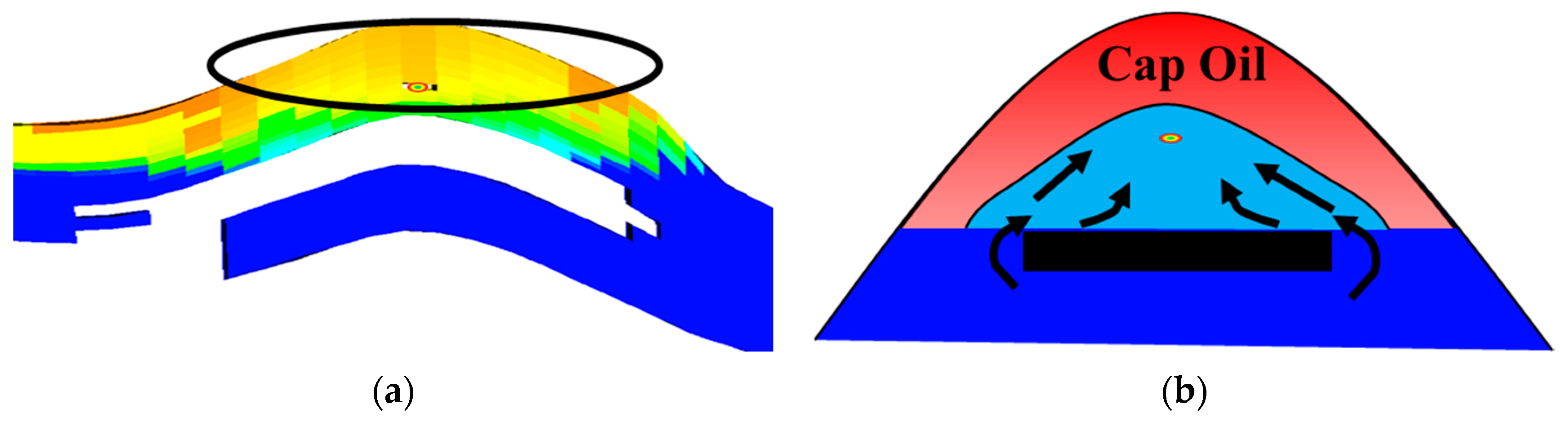
For the remaining oil controlled by interlayers, it can be mainly categorized into dome oil and bottom dome oil (as shown in Figure 6). The former refers to the remaining oil that has not been produced in the upper part of the interlayer. During the seepage process, the bottom water will be blocked by the interlayer, forming an unproduced cavity-shaped area in the upper part. Generally, the potential of the remaining oil is relatively small. The latter refers to the remaining oil formed below the interlayer, which is more like an inverted bell shape and has a relatively high remaining oil content. In the actual process of tapping the potential, due to the impermeable characteristics of the interlayer, it is very difficult to increase the flow velocity or flow rate. For both dome oil and bottom dome oil, the difficulty in tapping their potential is relatively high.
Figure 7a shows the cross-sectional view of residual oil distribution, while Figure 7b illustrates the schematic model of dome oil and bottom dome oil. The red areas in the figures represent the dome oil and bottom dome oil formed by interlayer barriers, which are challenging to be effectively extracted by existing production wells. Wells can hardly effectively produce them. Moreover, as development progresses, after the oil well starts to produce water, its swept area will also be relatively fixed. Therefore, certain measures must be taken to tap the potential of such remaining oil. Generally speaking, the methods of sidetracking old wells or drilling new infill wells have a relatively good effect on tapping the potential of this kind of remaining oil. Tapping the potential by increasing the liquid production and supplementing oil has a relatively limited effect. However, in the early stage, the method of increasing the liquid production can be adopted to increase the flow rate, expand the swept area, and improve the recovery degree. In the later stage, this method cannot be used to tap the potential.

4.3.2. Cap Oil

For the remaining oil jointly controlled by the structure and interlayers, it can be summarized as cap-shaped oil. Having structural highs, lower completion intervals, and developed interlayers are the conditions for its formation. Due to the existence of interlayers, secondary edge water drive is generated, which leads to the phenomenon of “hollowing out” at the bottom of the roof oil, thus forming the cap remaining oil.
As shown in Figure 8, remaining oil has been formed in the upper part of well, with Figure 8a illustrating the cross-sectional distribution of residual oil saturation and Figure 8b depicting the conceptual model of cap oil accumulation. Since it is difficult for the bottom water to sweep this area, the swept situation of this part of the area is limited. During the production process, it can only be produced under the action of reservoir pressure difference and gravity, and the production speed is slow. As the pressure at the bottom of the well stabilizes, its production degree will be even worse. Therefore, certain measures need to be taken to tap the potential. The tapping of the potential of cap-shaped remaining oil can mainly be achieved by increasing the liquid production of old wells, using the liquid to carry the oil, increasing the production pressure difference, and enlarging the drainage area. In addition, methods such as sidetracking old wells, drilling infill wells, and perforating passing wells can also be adopted to achieve effective control of the high structural positions, and then improve the production effect of the remaining oil at the structural highs. When deploying new wells in the early stage of oilfield development, it is also necessary to be as close as possible to the structural highs, make full use of the blocking effect of interlayers on the bottom water, improve the sweep coefficient of secondary edge water, and then ensure efficient development.

5. Conclusions

This study proposes an automatic interlayer identification method based on logging curve units and investigates remaining oil distribution. The key conclusions are as follows:
(1)
An automated interlayer identification framework was established by integrating multi-source logging data and dynamic activity-based layering methods. This framework achieves 90% interlayer identification accuracy, significantly improving efficiency over traditional manual interpretation. It provides an automated solution for quantitative characterization of reservoir heterogeneity. The method has been successfully applied to 3D interlayer modeling in the P Oilfield, demonstrating its engineering applicability.
(2)
The dominant controlling factors of remaining oil distribution were analyzed, revealing the impacts of small-scale interlayers and interlayer–structure interactions. Three typical remaining oil distribution patterns were identified: dome oil, bottom dome oil, and cap oil. These findings provide theoretical support for optimizing well placement and development strategies.
(3)
Future research will incorporate mineralogical data (e.g., thin-section analysis) and machine learning algorithms to enhance interlayer boundary prediction. This approach will be extended to reservoirs with complex diagenetic facies to achieve intelligent interlayer identification.

Author Contributions

Conceptualization, S.C., J.L. and Z.F.; methodology, Y.L.; validation, S.C., X.L. and Y.X.; formal analysis, Q.W.; investigation, J.L. and Y.L.; resources, Z.F. and M.S.; data curation, S.C.; writing—original draft preparation, S.C. and Y.X.; writing—review and editing, X.L. and Y.L.; visualization, M.S. and Q.W.; supervision, Q.W.; project administration, J.L.; funding acquisition, S.C. All authors have read and agreed to the published version of the manuscript.

Funding

The research was funded by China National Petroleum Corporation (CNPC) and China University of Petroleum (Beijing) (CUPB), under the Strategic Cooperation Technology Projects of CNPC and CUPB, with the grant number ZLZX2020-02-04. The APC was also funded by the Strategic Cooperation Technology Projects of CNPC and CUPB.

Data Availability Statement

Restrictions apply to the availability of these data. The data were obtained from PetroChina Changqing Oilfield Company and are available from the corresponding authors with the permission of PetroChina Changqing Oilfield Company.

Conflicts of Interest

Authors Shoumin Chen, Junjian Li, Yan Lei, Zhi Fan, Ma Suo and Qin Wang were employed by the company PetroChina Changqing Oilfield Company. The remaining authors declare that the research was conducted in the absence of any commercial or financial relationships that could be construed as a potential conflict of interest.

References

  1. Mahdi, T.A.; Aqrawi, A.A.M. Sequence Stratigraphic Analysis of the Mid-Cretaceous Mishrif Formation, Southern Mesopotamian Basin, Iraq. J. Pet. Geol. 2014, 37, 287–312. [Google Scholar] [CrossRef]
  2. Lin, C.; Hou, L.; Dong, C.; Zhang, J. Identification of interlayers using geostatistical methods: A case study of the third section of the Sha Formation in the western depression of the Liaohe River. Pet. Geol. Exp. 1997, 19, 245–251. [Google Scholar]
  3. Karp, J.C.; Lowe, D.K.; Marusov, N. Horizontal Barriers for Controlling Water Coning. J. Pet. Technol. 1962, 14, 783–790. [Google Scholar] [CrossRef]
  4. Huang, S.; Kang, B.; Cheng, L.; Zhou, W.; Chang, S. Quantitative Characterization of Interlayer Interference and Productivity Prediction of Directional Wells in the Multilayer Commingled Production of Ordinary Offshore Heavy Oil Reservoirs. Pet. Explor. Dev. 2015, 42, 533–540. [Google Scholar] [CrossRef]
  5. Makhatova, M.; Ozkan, E. A Practical Model for Pressure- and Rate-Transient Behavior of Stacked Horizontal Wells in Unconventional Reservoirs. In The Unconventional Resources Technology Conference; American Association of Petroleum Geologists: Houston, TX, USA, 2024. [Google Scholar] [CrossRef]
  6. Zhao, Q.; Li, X.-S.; Chen, Z.-Y.; Xia, Z.-M.; Xiao, C.-W. Numerical Investigation of Production Characteristics and Interlayer Interference during Co-Production of Natural Gas Hydrate and Shallow Gas Reservoir. Appl. Energy 2024, 354, 122219. [Google Scholar] [CrossRef]
  7. Tan, J.; Chen, J.; Zhang, Z.; Liu, C.; Zhang, W. Identification of Interlayer in Strong Bottom Water Reservoir and Its Influence on Development Effect. J. Geosci. Environ. Prot. 2022, 10, 132–138. [Google Scholar] [CrossRef]
  8. Luo, H.; Deng, H.; Xiao, H.; Geng, S.; Hou, F.; Luo, G.; Li, Y. A Transient-Pressure-Based Numerical Approach for Interlayer Identification in Sand Reservoirs. Fluid Dyn. Mater. Process. 2024, 20, 641–659. [Google Scholar] [CrossRef]
  9. Wu, Y.; Fan, Y.; Cai, L.; Fang, Z.; Li, C. Detection Performance and Grading-Selection-Based Inversion of Low-Frequency Alternating Current Resistivity Logging in Moderate-High Resistance Formations. SPE J. 2023, 28, 355–370. [Google Scholar] [CrossRef]
  10. Omrani, S.; Tavakoli, V. Influences of Geological and Petrophysical Attributes on Electrical Resistivity–Based Reserve Evaluation: Enhancing Carbonate Reservoir Classification, Permian-Triassic Reservoirs of Southern Iran. SPE J. 2024, 29, 5352–5371. [Google Scholar] [CrossRef]
  11. Figiel, M.; Lewandowska-Smierzchalska, J. Identification of Strata from Irregularities in Well Logs Using Chaos Quantifiers. SPE J. 2022, 27, 1770–1781. [Google Scholar] [CrossRef]
  12. Jarzyna, J.A.; Bala, M.J.; Mortimer, Z.M.; Puskarczyk, E. Reservoir Parameter Classification of a Miocene Formation Using a Fractal Approach to Well Logging, Porosimetry and Nuclear Magnetic Resonance. Geophys. Prospect. 2013, 61, 1006–1021. [Google Scholar] [CrossRef]
  13. Hill, E.J.; Uvarova, Y. Identifying the Nature of Lithogeochemical Boundaries in Drill Holes. J. Geochem. Explor. 2018, 184, 167–178. [Google Scholar] [CrossRef]
  14. Xu, C.; Bayer, W.S.; Wunderle, M.; Bansal, A. Normalizing Gamma-Ray Logs Acquired from a Mixture of Vertical and Horizontal Wells in the Haynesville Shale. Petrophysics—SPWLA J. Form. Eval. Reserv. Descr. 2016, 57, 638–643. [Google Scholar]
  15. Schlanser, K.; Grana, D.; Campbell-Stone, E. Lithofacies Classification in the Marcellus Shale by Applying a Statistical Clustering Algorithm to Petrophysical and Elastic Well Logs. Interpretation 2016, 4, SE31–SE49. [Google Scholar] [CrossRef]
  16. Maalouf, E.; Torres-Verdin, C. Interpretation of Borehole Sonic Measurements Acquired in Vertical Transversely Isotropic Formations Penetrated by Vertical Wells. Geophysics 2018, 83, D187–D202. [Google Scholar] [CrossRef]
  17. Han, M.; Li, G.; Chen, J. Assimilating Microseismic and Well-Test Data by Use of EnKF for Accurate Reservoir Characterization. SPE J. 2015, 20, 186–201. [Google Scholar] [CrossRef]
  18. Zhang, L.; Li, R.; Deng, H.; Fu, M.; Hu, L.; Guo, X.; Xie, X.; Zhao, C. Identification, Distribution Characteristics, and Effects on Production of Interlayers in Carbonate Reservoirs: A Case Study from the Cretaceous Mishrif Formation in Halfaya Oilfield, Iraq. J. Pet. Sci. Eng. 2021, 202, 108571. [Google Scholar] [CrossRef]
  19. Bhattacharya, S.; Carr, T.R. Integrated Data-Driven 3D Shale Lithofacies Modeling of the Bakken Formation in the Williston Basin, North Dakota, United States. J. Pet. Sci. Eng. 2019, 177, 1072–1086. [Google Scholar] [CrossRef]
  20. Fu, C.; Xie, Y.; Wang, H.; Song, L.; Duan, R.; Yuan, Z.; Xu, W.; Chen, G. Types and Sedimentary Genesis of Barriers and Interlayers in the Composite Turbidite Sand Bodies of a Deep-Water Canyon: A Case Study of the Central Canyon in the Qiongdongnan Basin. Nat. Gas Ind. B 2023, 10, 511–521. [Google Scholar] [CrossRef]
  21. Yi, J.; Li, H.; Shan, X.; Hao, G.; Yang, H.; Wang, Q.; Xu, P.; Ren, S. Division and Identification of Vertical Reservoir Units in Archaeozoic Metamorphic Buried Hill of Bozhong Sag, Bohai Bay Basin, East China. Pet. Explor. Dev. 2022, 49, 1282–1294. [Google Scholar] [CrossRef]
  22. Li, F.; Li, Y.; Chen, J.; Li, L.; Ren, L.; Meng, L.; Wang, W.; Wan, Y.; Lu, Y.; Chen, H. Methods of Division of Development Unit for Thick Carbonate Reservoir—A Case Study of the Mishrif Formation, a Oilfield, Middle East. Geofluids 2024, 2024, 7361600. [Google Scholar] [CrossRef]
  23. Singh, H.; Seol, Y.; Myshakin, E.M. Automated Well-Log Processing and Lithology Classification by Identifying Optimal Features through Unsupervised and Supervised Machine-Learning Algorithms. SPE J. 2020, 25, 2778–2800. [Google Scholar] [CrossRef]
  24. Liu, H.; Peng, S.; Xia, H.; Tang, H. Mathematic characteristics of Well LoggingCurve Unit and quantitative identification of sedimentary miscrofacies. China Offshore Oil Gas 2004, 16, 45–50. [Google Scholar]
  25. Zhang, Q.; Ge, Y.; Li, Y. Automatic interlayer identification method based on gradient and Bayesian discriminant method. J. Heilongjiang Univ. Sci. Technol. 2015, 25, 177–181. [Google Scholar]
  26. Yi, J. Automatic Geologic Zonation Using Activity Layering Method. J. Oil Gas Technol. 2007, 29, 78–81. [Google Scholar]
  27. Wang, J.; Liu, H.; Xu, J.; Zhang, H. Formation Mechanism and Distribution Law of Remaining Oil in Fracture-Cavity Reservoir. Pet. Explor. Dev. 2012, 39, 624–629. [Google Scholar] [CrossRef]
  28. Ghazi, S.; Mountney, N.P. Facies and Architectural Element Analysis of a Meandering Fluvial Succession: The Permian Warchha Sandstone, Salt Range, Pakistan. Sediment. Geol. 2009, 221, 99–126. [Google Scholar] [CrossRef]
  29. Munawar, M.J.; Lin, C.; Chunmei, D.; Zhang, X.; Zhao, H.; Xiao, S.; Azeem, T.; Zahid, M.A.; Ma, C. Architecture and Reservoir Quality of Low-Permeable Eocene Lacustrine Turbidite Sandstone from the Dongying Depression, East China. Open Geosci. 2018, 10, 87–112. [Google Scholar] [CrossRef]
  30. Xue, Y.; Cheng, L. The Influence of Interlayer of Bottom Water Reservoirs during the Development Stage. Pet. Sci. Technol. 2013, 31, 849–855. [Google Scholar] [CrossRef]
  31. Zhao, L.; Liang, H.; Zhang, X.; Chen, L.; Wang, J.; Cao, H.; Song, X. Relationship between Sandstone Architecture and Remaining Oil Distribution Pattern: A Case of the Kumkol South Oilfield in South Turgay Basin, Kazakstan. Pet. Explor. Dev. 2016, 43, 474–483. [Google Scholar] [CrossRef]
  32. Liu, T.; Fawad, N.; Li, C.; Li, H.; He, R.; Xu, J.; Ahmad, Q.A. Physical Simulation of Remaining Oil Distribution in the 3rd-Order Architecture Unit in Beach Sand Reservoir. Front. Earth Sci. 2023, 10, 1108525. [Google Scholar] [CrossRef]
  33. Feng, C.; Bao, Z.; Yang, L.; Si, X.; Xu, G.; Han, X. Reservoir Architecture and Remaining Oil Distribution of Deltaic Front Underwater Distributary Channel. Pet. Explor. Dev. 2014, 41, 358–364. [Google Scholar] [CrossRef]
  34. Chen, X.; Xiao, P.; Duan, R.K.; Lv, W.R.; Zhang, X.; Chen, G.N. Study on flow unit division and remaining oil tapping in deep-water turbidite gas injection reservoir. Unconv. Oil Gas 2023, 10, 103–111. [Google Scholar]
  35. Xie, P.; Yin, Y.; Li, W.; Li, F.; Zhao, L. Distribution of Remaining Oil Based on a Single Sand Body Analysis: A Case Study of Xingbei Oilfield. J. Pet. Explor. Prod. Technol. 2018, 8, 1159–1167. [Google Scholar] [CrossRef]
  36. Sun, P.; Fang, H.; Xu, Z.; Wang, C.; Xu, H.; Lu, M. Siliciclastic Depositional Model within a Subsurface Coastal Parasequence Based on Barriers and Baffles—An Application to the Donghe Sandstone Member in the Hudson Oilfield, Tarim Basin, NW China. J. Pet. Sci. Eng. 2020, 195, 107947. [Google Scholar] [CrossRef]
  37. Han, R.; Liu, Q.; Jiang, T.; Xu, H.; Xu, Z.; Zhao, L.; Lei, C.; Zhang, P. Feature, Origin and Distribution of Calcareous Interlayers: A Case of Carboniferous Donghe Sandstone in Hade Oil Field, Tarim Basin, NW China. Pet. Explor. Dev. 2014, 41, 475–484. [Google Scholar] [CrossRef]
  38. Gao, Y.; Zhang, X.; Zhang, L.; Wu, Z.; Lao, M.; Li, H.; Wu, T. Geological Characteristics and Tectonic Settings of Mesozoic Continental Margin Magmatic Arc in Pearl River Mouth Basin. Earth Sci. 2022, 47, 2317–2327. [Google Scholar] [CrossRef]
  39. Zhang, J.; Yan, D.; Zhou, S.; Wang, H.; Deng, Y.; Liu, E.; Song, G. Sedimentological and Diagenetic Effects on Petrophysical Characteristics and Hydraulic Flow Units of Zhujiang Sandstones in the Pearl River Mouth Basin, South China Sea. Energy 2023, 282, 128942. [Google Scholar] [CrossRef]
  40. Wu, T.; Zhang, L.; Wu, Z.; Li, H.; Lei, S.; Yu, S.; Lao, M. Characteristics and dynamic background of pre-existing fractures in pre-Cenozoic of Pearl River Mouth Basin: Cases of Huizhou Sag and Panyu 4 Depression. Marine Geol. Front. 2022, 38, 54–62. [Google Scholar] [CrossRef]
  41. Chang, M.; Deng, R.; Wang, H.; Xie, B.; Zhao, Z. Research on the Normalisation Method of Logging Curves: Taking XJ Oilfield as an Example. Appl. Math. Nonlinear Sci. 2021, 6, 99–110. [Google Scholar] [CrossRef]
  42. Wang, L.; Xiong, Q.; Jiang, Q.; Wang, Z.; Qiu, Z.; Liu, K.; Kong, C.; Liu, C.; Zhang, X. Correction Method for Logging Curves in Clay-Rich Tight Glutenite Reservoir: Upper Wuerhe Formation in Mahu Oilfield, China. Energies 2022, 15, 7119. [Google Scholar] [CrossRef]
  43. Wang, X.; Hou, J.; Liu, Y.; Ji, L.; Sun, J. Studying Reservoir Heterogeneity by Analytic Hierarchy Process and Fuzzy Logic, Case Study of Es1x Formation of the Wang Guan Tun Oilfield, China. J. Pet. Sci. Eng. 2017, 156, 858–867. [Google Scholar] [CrossRef]
Figure 1. Core images of calcareous interlayers (a) and argillaceous interlayers (b).
Processes 13 00425 g001
Figure 2. Secondary fine logging interpretation chart.
Processes 13 00425 g002
Figure 3. Multi-well interlayer distribution profile (The black lines represent the sublayers, and the gray areas represent the interlayers).
Processes 13 00425 g003
Figure 4. Planar distribution patterns of interlayers within sublayers; (ac) represent different sublayers in the P Oilfield.
Processes 13 00425 g004
Figure 5. Oil saturation field map of a sublayer after five years of production. (a) Oil saturation field map. (b) Cross-sectional profile. (a), the red lines represent the trajectories of the horizontal wells. The red ellipses in both (a,b) correspond to the same region, indicating the areas of remaining oil accumulation.
Processes 13 00425 g005
Figure 6. Oil saturation field map of another sublayer after five years of production. (a) Oil saturation field map. (b) Cross-sectional profile. (a), the red lines represent the trajectories of the horizontal wells. The red ellipses in both (a,b) correspond to the same region, indicating the areas of remaining oil accumulation.
Processes 13 00425 g006
Figure 7. Remaining oil distribution characteristic map. (a) Remaining oil cross-sectional profile. (b) Dome oil and bottom dome oil pattern map. (a) the black ellipse indicates the region where Dome Oil and Bottom Dome Oil are located within the reservoir numerical model. (b) the black arrows represent the direction of water movement, and the red area denotes the remaining oil.
Processes 13 00425 g007
Figure 8. Remaining oil distribution characteristic map. (a) Remaining oil cross-sectional profile. (b) Cap oil pattern map. (a) the black ellipse indicates the region where Cap Oil are located within the reservoir numerical model. (b) the black arrows represent the direction of water movement, and the red area denotes the remaining oil, the light blue and dark blue areas both represent the bottom water of the reservoir.
Processes 13 00425 g008
Table 1. Identification results of interlayers with different critical values (partial).
ThresholdManually Identified
Interlayer Number
Automatically Identified
Interlayer Number
Error
0.5563108793.07%
0.5556394668.03%
0.656380342.63%
0.6556369122.74%
0.75635713.55%
0.75563551−2.13%
0.8563403−28.42%
0.85563381−32.33%
0.9563129−77.09%
Table 2. Identification results of interlayers in well A1 (partial).
NumberTop Depth of Curve UnitBottom Depth of Curve Element P l Interlayer Development Status
11609.21610.50.591Sandstone section
21610.51611.70.565Sandstone section
31611.71613.10.767Interlayer development
41613.11615.90.579Sandstone section
51615.91618.50.891Interlayer development
61618.51620.80.224Sandstone section
71620.81623.10.149Sandstone section
81623.11624.90.155Sandstone section
91624.91626.20.079Sandstone section
101626.21628.00.425Sandstone section
111628.01629.30.547Sandstone section
121629.31630.70.548Sandstone section
131630.71631.90.737Interlayer development
141631.91634.90.829Interlayer development
Table 3. Physical properties of the numerical model of the target oilfield.
ThresholdManually Identified
Interlayer Number
Automatically Identified Interlayer Number
Reservoir CharacteristicsReservoir Burial Depth (m)−1438~−1822
Initial Formation Pressure (MPa)14.7~18.1
Saturation Pressure (MPa)0.207~0.752
Reservoir Temperature (°C)68.2~82.2
Permeability (10−3 μm2)1255.8~6042.7
Porosity (%)21.5~31.5
Rock Compressibility Coefficient (MPa−1)4.859
Fluid
Characteristics
Surface Crude Oil Density (g/cm3)0.90~0.96
Formation Crude Oil Viscosity (mPa·s)31.71~137.98
Initial Solution Gas–Oil Ratio (m3/m3)0.03~1.07
Crude Oil Volume Factor1.037~1.043
Crude Oil Compressibility Coefficient (MPa−1)7.73 × 10⁻⁴~1.03 × 10⁻³
Water Density (g/cm3)1.029
Water Viscosity (mPa·s)0.3
Water Compressibility Coefficient (MPa−1)4.375 × 10⁻⁴
Gas Relative Density0.86~1.35
Disclaimer/Publisher’s Note: The statements, opinions and data contained in all publications are solely those of the individual author(s) and contributor(s) and not of MDPI and/or the editor(s). MDPI and/or the editor(s) disclaim responsibility for any injury to people or property resulting from any ideas, methods, instructions or products referred to in the content.

