Abstract
To address the dynamic characteristics of data collection, risk assessment, and response execution in intelligent traffic warning systems, this study proposes a modeling and performance analysis framework based on Stochastic Petri Nets (SPN). An SPN model of the warning-information evolution process is constructed and transformed into a continuous-time Markov chain (CTMC), for which the steady-state probability equations are derived to quantify system performance. The transition rates in the model are assigned according to national technical specifications and practical operational scenarios. A sensitivity analysis is conducted on several key rates (λ2, λ3, λ9, λ10, λ11, λ12) to examine their influence on the steady-state distribution. The simulation results indicate that increasing λ2 (data-cleaning rate) improves processing efficiency in the data-fusion stage, while insufficient values of λ10 or λ11 may lead to system congestion or delayed responses. To further evaluate system behavior, performance indicators such as the average number of tokens and transition utilization are introduced to assess resource occupancy and process activation frequency. These measures help identify potential bottlenecks and guide targeted optimization. The findings demonstrate that appropriate adjustment of critical transition rates can enhance operational efficiency and warning accuracy, providing theoretical support and practical insights for the modeling, optimization, and resource allocation of intelligent traffic systems.
1. Introduction
Intelligent Transportation Systems (ITSs) rely on well-developed infrastructure such as roads, ports, airports, and communication networks. By integrating advanced information technologies—including data communication and transmission, electronic sensing and monitoring, electronic control, and computer processing—ITS supports the development of a real-time, accurate, and efficient transportation management framework with comprehensive operational coverage [1,2] ITS also transforms the traditional interaction model among the three core elements of transportation systems: people, vehicles, and roads. With the deployment of ITS, road utilization can be improved, vehicle energy consumption can be reduced, traffic congestion can be alleviated, short-distance mobility efficiency can be enhanced, and the capacity of existing road networks can be strengthened [3]. After more than a decade of promotion, testing, and development, ITS has been widely implemented in both urban and highway networks across developed and developing countries. Practical experience has demonstrated that ITS provides an effective response to the transportation pressures driven by rapid economic growth [4]. Intelligent traffic early warning systems play an important role in accident prevention, rapid response, and the efficient use of road resources, and therefore remain a central research topic within Intelligent Transportation Systems (ITSs). To support early warning and safety management in transportation infrastructures, several studies have explored the integration of sensing, monitoring, and simulation technologies. For example, Wu Xianguo et al. [5] developed an IoT-based structural health monitoring framework for subways using BIM technology, which enabled the visualization of structural monitoring data. Gaofeng and colleagues [6] combined BIM with GIS to examine its application in safety forecasting and early warning for subway tunnels. Zhang Jianqing [7] designed a temperature monitoring and warning system for high-speed railway ballastless tracks, capable of computing and predicting temperature distributions. In a different context, Quan Xiongwei and Zuo Gaoshan [8] investigated NIMBY conflicts associated with waste-to-energy plants by constructing an evolutionary model based on Stochastic Petri Nets (SPN). Drawing on grounded theory and multiple real-world cases, they identified eleven categories of influencing factors, including risk perception, government trust, and experiential cognition. Their study established the SPN structure and its isomorphic Markov chain, and derived the steady-state probability distribution to characterize the long-term evolution of residents’ collective behavioral states. Sensitivity simulations on key transition rates (e.g., λ2, λ7, λ12) further revealed how government decision-making, information dissemination, and opinion-leader mobilization affect protest dynamics and conflict escalation. This work highlights the capability of SPN models to capture the evolution of social group behaviors and provides quantitative insights for conflict prevention and policy intervention. An efficient crisis early warning mechanism is essential for managerial decision-making, effective governance, and improved resource utilization [9]. Existing research on early warning systems can generally be categorized into three areas. The first area is early warning identification, which applies methods such as convolutional neural networks, bipartite and relational networks, graph embedding techniques, and graph2vec algorithms to extract risk features from raw data, identify risk propagation paths, and detect critical targets. These approaches significantly enhance the accuracy of early warning processes.
The second area is early warning monitoring. Techniques such as scan statistics and conditional random field-based risk classification models are used to detect the onset of crisis events and support the dynamic monitoring of public opinion-related risks The third area is early warning assessment, in which big data analytics and computational experiments are employed to strengthen data-driven decision-making and improve the evaluation of crisis risk levels.
The core of a crisis early warning mechanism lies in the selection of warning indicators and the design of appropriate forecasting methods. In terms of indicator development, Yang Xiaoxi et al. [10], drawing on information ecology theory, mapped the relationships among information ontology, information environment, information agents, and public opinion onto constructs such as information niche breadth, information proliferation state, and competition–cooperation dynamics. This mapping provided a systematic basis for building an early warning indicator system. Huang Wei [11] examined the causes, development, and consequences of online terrorist incidents, proposing a corresponding indicator framework and identifying early-stage online popularity and influence as the most critical predictive factors. In terms of predictive methods, Tian Shihai [12] developed crisis early warning indicators based on the information attributes of online public opinion during emergencies and constructed a three-level risk index system (Levels I–III). He further designed a “stepwise-parallel” early warning mechanism by embedding these indices into a structured decision framework and applied it to the “Beijing Xinfadi COVID-19 outbreak,” where the mechanism was simulated using the isomorphism between Stochastic Petri Nets (SPN) and Markov chains. Additionally, Huang Jing [13] analyzed agricultural drought emergency management using the OODA loop model, established a multi-department collaborative response process, and constructed an SPN-based simulation model. Performance analysis of the corresponding Markov chain revealed key process stages and opportunities for optimizing processing times. Although these studies provide valuable methodological insights, they fall short in offering a clear and intuitive representation of the operational dynamics underlying crisis early warning systems.
With the increasing complexity and dynamism of modern urban transportation systems, research attention has increasingly shifted toward modeling and analyzing their stochasticity, concurrency, and real-time responsiveness. Traditional modeling approaches [12,13,14,15], such as differential equations and Markov chains, can describe certain dynamic behaviors but are limited in capturing concurrent events, resource competition, and system-level uncertainties. Stochastic Petri Nets (SPNs), which combine probability theory with parallel computation, offer a more expressive modeling framework for performance evaluation and optimization. In an SPN, places represent local system states, transitions represent state-changing events, and arcs define their relationships through input and output connections [16]. Leveraging the dynamic descriptive capabilities of SPNs, researchers have quantified state transition probabilities in complex evolutionary processes, identified system bottlenecks, and optimized resource allocation to enhance operational performance. In an SPN model, places may contain any number of tokens that represent the evolving state of the system. As events occur, tokens move among places according to the direction of arcs, thereby capturing real-time state transitions. The dynamic behavior of an SPN is governed by its firing rules. Each transition has a set of input places and output places. A transition becomes enabled when all its input places contain at least the required number of tokens specified on the input arcs. Once enabled, the transition fires after a stochastic delay. The firing process removes tokens from input places and simultaneously generates tokens in the output places, forming an atomic, indivisible update step. The time-varying distribution of tokens across places is known as the marking, which represents the current system state [16]. The concept of the Petri Net was first introduced by Carl Adam Petri in 1962. Since the first international workshop in 1980, the theoretical foundations and applications of Petri Nets have undergone significant development. Various extensions have been proposed to address the growing complexity of modern systems. For example, the Generalized Stochastic Petri Net (GSPN) simplifies state-space structures; the Extended Stochastic Petri Net (ESPN) supports non-exponential firing distributions; the Deterministic and Stochastic Petri Net (DSPN) combines deterministic delays with discrete-time Markov chains; the Stochastic Reward Net (SRN) incorporates reward structures for performance evaluation; and the Stochastic High-Level Petri Net (SHLPN) integrates exponentially distributed timing into high-level constructs [16]. Due to its adaptability in modeling complex systems, the SPN framework has been widely applied to simulate the evolution of group events, infectious disease transmission, and network information propagation. These studies often emphasize sensitivity analysis of critical transition parameters. In the field of intelligent transportation, SPN research has also made substantial progress. For instance, Zhong Xianxin [17] extended the ROAD meta-architecture into the ROADS framework to overcome the limitations of traditional IDEF0-based activity models in representing complex triggers and information-exchange scenarios. Huang Fenglan [18] further proposed a method for generating executable Colored Petri Net (CPN) models from TOGAF business architectures by mapping the four categories defined in the ACF meta-model—Rule Model (RM), Organization Model (OM), Activity Model (AM), and Data Model (DM)—to CPN constructs and formulating a five-stage modeling process. While prior works such as Zhong et al. and Huang et al. have advanced executable and architecture-oriented Petri net modeling for business and data-flow mapping, these approaches primarily focus on automated model generation and architecture-to-CPN translations rather than on targeted subprocess-level sensitivity analysis. In contrast, this study explicitly constructs a modular SPN organized around the perception–decision–response loop, where each transition rate (λ) is mapped to a clearly identifiable operational subprocess (e.g., data-cleaning, early-warning evaluation). Yan Zhe [19] incorporated the four elements of game theory into Logical Petri Nets and applied a Logical Game Probabilistic Petri Net to model subway emergency decision-making processes. Li Jingyu et al. [20] provided theoretical support for traffic signal coordination control. Huang Fenglan [21] also introduced a Hierarchical Colored Petri Net (HCPN) with arc weights to formalize data flow representation while modeling multi-instance and sub-process structures. Sun Qipeng [22] employed the Visual Object Net++ simulation platform to construct and simulate an SPN model of the intercity passenger travel service process, further transforming it into an isomorphic Markov chain to analyze urban subway travel as a sub-process, thereby optimizing intercity passenger services. In related research on human–robot collaboration (HRC) for complex task allocation, Xiao et al. [23] proposed a multi-scenario digital twin-driven HRC multi-task disassembly process planning framework, based on dynamic Time Petri Net (TPN) models and a heterogeneous multi-agent double deep Q-learning network. Their approach integrates TPN models to represent real-time disassembly information and relationships, while the multi-agent learning algorithm determines optimal disassembly sequences and task allocations. Similarly, Xiao [24] developed an improved HRC disassembly method combining Q-learning with Particle Swarm Optimization (PSO) to optimize multi-agent disassembly task sequences for electric vehicle battery recycling. This method further integrates Q-learning with a variable neighborhood search (VNS) algorithm to enhance local search capabilities and improve task allocation efficiency. Case studies on battery disassembly demonstrate that these approaches significantly improve the efficiency and flexibility of HRC task planning under dynamic operational conditions. Together, these studies illustrate the potential of Petri net-based and reinforcement learning-enhanced frameworks to optimize complex, uncertain, and multi-agent systems, providing a conceptual parallel to SPN-based performance modeling in intelligent traffic systems. In addition to stochastic Petri nets, fuzzy logic-based approaches have been widely investigated for adaptive urban traffic control. Jafari (2021) [25] proposed a Takagi–Sugeno (TS) fuzzy controller that adjusts traffic signals based on queue lengths and vehicle flow at intersections, using state-space modeling to capture waiting times and queue dynamics. Stability was verified through Lyapunov analysis, and simulations showed improvements over conventional fuzzy and fixed-time controllers. Similarly, Tunc (2021) [26] implemented a fuzzy logic controller for a four-legged junction, where the inputs included queue length and vehicle location state. Using the Simulation of Urban Mobility (SUMO) platform, the authors demonstrated that adaptive signal timing reduces waiting times and queue lengths compared with static approaches. While fuzzy logic controllers excel at handling uncertainty and providing flexible local control, stochastic Petri nets (SPNs) offer a complementary system-level perspective. SPNs explicitly represent discrete events, concurrent processes, and probabilistic behaviors, which allow for performance evaluation, reliability analysis, and the identification of system bottlenecks in complex, multi-layered intelligent transportation scenarios. Building on the development of fuzzy logic and reinforcement learning approaches, agent-based modeling (ABM) has also emerged as a powerful alternative for simulating complex transportation systems. Chen Gao (2023) [27] surveyed the integration of large language models into ABM, highlighting their potential to enhance environment perception, agent decision-making, and scenario evaluation. Furthermore, Bastarianto (2023) [28] proposed an adaptive traffic signal control framework using ABM to model heterogeneous vehicle behaviors and dynamic interactions at intersections, demonstrating the method’s effectiveness in reducing congestion and improving traffic flow. While ABM focuses on modeling individual agents and their interactions to capture emergent behaviors, stochastic Petri nets (SPNs) provide a complementary system-level perspective, explicitly representing concurrent events, probabilistic behaviors, and state transitions. Combining insights from both approaches can offer a more comprehensive understanding of adaptive traffic control and system performance under uncertainty.
The main contributions of this work are as follows: (1) it proposes a modular SPN representation of the intelligent traffic warning process, explicitly structured around the perception–decision–response loop. This design enables clear separation and interaction modeling of acquisition, judgment, and response subprocesses. (2) It develops a mapping scheme that links SPN transition rates to domain-specific performance metrics, making sensitivity analysis directly applicable to resource allocation and workflow redesign. (3) It integrates steady-state probabilities with additional operational indicators—average token counts and transition utilization rates—to more precisely identify bottlenecks. (4) It introduces a state-reduction procedure that preserves functional semantics while mitigating state-space explosion, ensuring tractable steady-state analysis for applied scenarios.
2. Intelligent Traffic Warning Process
2.1. Definition of Intelligent Traffic Warning Mechanism
Within intelligent transportation systems, different alert levels correspond to traffic incidents of varying severity. In this study, red and orange alerts represent high-risk and medium-risk traffic events, respectively, and are defined as follows.
Red Alerts (high risk, requiring urgent response):
These alerts are triggered by major traffic incidents such as multi-vehicle collisions and serious crashes; road closures caused by infrastructure failures (e.g., bridge or tunnel collapses); traffic disruptions resulting from extreme weather conditions (including heavy snow, rainstorms, and typhoons); large-scale congestion where major arterial roads remain blocked beyond predefined thresholds; hazardous materials incidents such as chemical or fuel leaks; and severe traffic violations, including drunk driving or driving against traffic on highways.
Orange Alerts (moderate risk, requiring early intervention):
These alerts correspond to moderate-scale traffic events such as single-vehicle guardrail impacts or two-vehicle collisions; localized congestion limited to a specific road segment; adverse but non-extreme weather conditions (e.g., heavy fog, showers, or icy road surfaces); equipment failures including traffic signal malfunctions or monitoring system anomalies; and minor traffic violations such as illegal parking or failing to obey traffic signals.
Clarifying the definitions of these alert levels enables a more detailed analysis of the probability of different types of incidents and supports the optimization of intelligent traffic management strategies.
2.2. Adaptability of the Architecture of Intelligent Traffic Warning Systems and Stochastic Petri Net Modeling
The intelligent transportation early-warning system operates around the core loop of perception–decision–response, whose inherent dynamics and complexity can be efficiently captured through Stochastic Petri Nets (SPNs). Characterized by concurrency, randomness, and selectivity, intelligent transportation warning processes align closely with the modeling strengths of SPNs. Specifically, SPNs intuitively represent the system’s states and events, while transition rates (λ) quantify processing delays and judgment latencies, thereby enabling rigorous performance evaluation. Moreover, SPNs can be mapped to isomorphic Markov chains, which support steady-state probability analysis and performance assessment. By calibrating λ parameters against empirical standards, the model’s applicability to real-world transportation systems is further reinforced.
In this regard, innovative approaches to intelligent transportation underscore the scalability of SPNs in modeling complex traffic systems, particularly in scenarios involving high concurrency and stochastic events. This provides not only a theoretical foundation but also practical insights for intelligent traffic management in the context of global smart cities. As illustrated in Figure 1, the system initiates with data acquisition, followed by sequential stages of processing and analysis, traffic condition detection, management and emergency response, and ultimately the dissemination of warning information. Data sources include GPS, roadside sensors, and in-vehicle cameras. After preprocessing and validation, the system determines data availability and, based on real-time traffic signal conditions, executes adaptive control and scheduling. Finally, the system issues intervention measures corresponding to the assessed warning levels, thereby optimizing traffic flow and reducing accident risks.
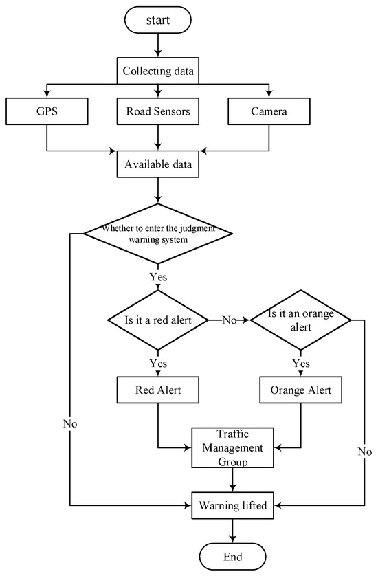
Figure 1.
Intelligent Traffic Early Warning System Flowchart.
3. Intelligent Traffic Warning Model Based on Random Petri Net
3.1. Introduction to Random Petri Nets
Stochastic Petri Nets (SPNs) are an extension of Place/Transition (P/T) systems. To ensure that SPN models exhibit the same dynamic behavior as their underlying P/T counterparts, it is required that both models share identical potential firing sequences. This condition is achieved by associating each transition in the SPN with a random firing time, modeled as a stochastic variable. Such an extension enables Petri nets not only to capture the structural relationships between events but also to simulate the temporal distribution of their occurrences. SPNs have thus evolved into a powerful framework for describing and analyzing discrete-event systems with inherent randomness, such as event timing and probabilistic occurrences. By integrating the structured representation of Petri nets with the probabilistic rigor of stochastic processes, SPNs have found wide applications in system modeling, queuing networks, reliability analysis, and performance evaluation.
It has been formally demonstrated that every SPN is isomorphic to a Continuous-Time Markov Chain (CTMC). Specifically, each reachable marking in an SPN corresponds to a state in the Markov chain, and the transition process among markings can be mapped directly to state transitions in the CTMC. By constructing the isomorphic Markov chain, the reachability graph of the SPN can be transformed into the corresponding state-space structure. Moreover, the transition rate matrix of the CTMC can be readily derived from the SPN’s reachability graph, making it possible to compute the steady-state probabilities of each state (marking). These steady-state probabilities provide the foundation for performance analysis of SPN models [16].
An SPN is generally defined as a directed graph composed of six fundamental elements: SPN = (, in [16]:
- (1)
- P = {P0,P1, …, Pn} is a finite set of key elements in the evolution of traffic warning information, n > 0 the number of elements;
- (2)
- is a set of transitions in a dynamic system, indicating the time required for key elements to change from one state to another during the operation of each link in the evolution of traffic warning information;
- (3)
- is a directed arc set representing the flow relationship of information evolution direction, represented by a directional arrow;
- (4)
- is the arc weight function, assigning weights to directed arcs, ;
- (5)
- {0, 1, ⋯} is a set of identifiers; it is a vector that represents the possible states in the evolution process of traffic warning information; is the initial logo, and represents the initial state of the model;
- (6)
- λ = {λ0, λ1, ⋯, λn} is the set of transition firing rates of the elements of the traffic warning information evolution system, which is associated with time transitions. Time transitions obey a negative exponential distribution and represent the parameters of the distribution function.
3.2. SPN Model for Intelligent Traffic Warning Information Evolution
Due to the isomorphism between SPN and continuous-time Markov chains (CTMCs), this study employs the stationary distribution of a Markov chain to analyze the evolution of the intelligent traffic early-warning information system. The modeling process can be summarized in the following steps:
Step 1: As illustrated in Figure 1, the big data processing workflow for the intelligent traffic early warning system is mapped into the SPN model, where time-delayed operations are represented as corresponding timed transitions.
Step 2: Using the constructed SPN structural model (Figure 2), the reachable state set is analyzed, and the average firing rate of each transition is labeled on the corresponding arcs. Based on the transition relationships among state markings, an equivalent Markov chain is then established to assess the model’s liveness and boundedness. All possible states of the SPN model are denoted as M0, M1, M2, …, Mn, where n represents the total number of markings or states. Step 3: Based on the reachable state set obtained in Step 2, a Markov chain is constructed (Figure 3) that is isomorphic to the SPN model.
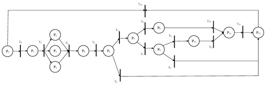
Figure 2.
SPN Model of Intelligent Traffic Early Warning.
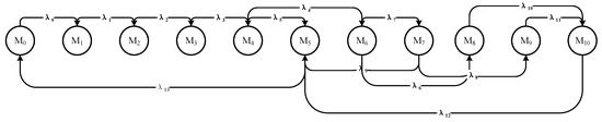
Figure 3.
Markov Chain Isomorphic Graph.
Step 4: By utilizing PIPE software (Platform Independent Petri Net Editor), version 4.3.0, the average number of tokens and their 95% confidence intervals are calculated. The busy states of the system are then analyzed, and the critical places are identified according to their average token occupancy.
Step 5: Based on the critical places identified in Step 4, transition firing rates are adjusted to observe the variation in steady-state probabilities under different scenarios, enabling system optimization.
The specific procedure is as follows: first, the SPN model is constructed (as illustrated in Figure 2). The places and transitions of the SPN are then symbolically defined, as shown in Table 1 and Table 2.

Table 1.
SPN Model Place Symbol Definition.
Table 2.
SPN Model Transition Symbol Definition.
The initial identification of the information evolution SPN model of the traffic warning is M0 = (1,0,0,0,0,0,0,0,0,0,0,0,0), The initial place P0 has a token. Therefore, we can derive the reachable sets caused by different transitions, and thus derive the following notations:
M1 = (0,1,0,0,0,0,0,0,0,0,0,0,0)
M2 = (0,0,1,1,1,0,0,0,0,0,0,0,0)
M3 = (0,0,0,0,0,1,0,0,0,0,0,0,0)
M4 = (0,0,0,0,0,0,1,0,0,0,0,0,0)
M5 = (0,0,0,0,0,0,0,0,0,0,0,0,1)
M6 = (0,0,0,0,0,0,0,1,0,0,0,0,0)
M7 = (0,0,0,0,0,0,0,0,1,0,0,0,0)
M8 = (0,0,0,0,0,0,0,0,0,1,0,0,0)
M9 = (0,0,0,0,0,0,0,0,0,0,1,0,0)
M10 = (0,0,0,0,0,0,0,0,0,0,0,1,0)
The traffic early-warning information evolution model, based on the SPN structure, contains 11 reachable states denoted as M0, M1, …, M10. During the modeling process, a continuous-time SPN can be transformed into a Markov chain through state mapping, where each SPN marking corresponds to a state in the Markov chain. The reachability graph of the SPN is isomorphic to the state space of the Markov chain.
According to the state-marking matrix derived from the SPN model, no state space explosion was observed, and the SPN is bounded. Based on the transitions in the state-marking graph, the isomorphic Markov chain was obtained, as illustrated in Figure 3.
Assume that the stable state probability of n states in MC is a row vector ;
All continuous-time stochastic Petri nets (SPNs) with a finite number of positions and transitions can be converted into one-dimensional continuous-time Markov chains (CTMCs) corresponding to their structures. According to the Markov process, we have the following linear equations:
According to the Markov process principle, there is the following stationary equation [24]:
Let P(Mi), be the stability probability of Mi in the equilibrium state of the Markov chain, then we can obtain the equation group:
By solving the above system of linear equations, the steady-state probability distribution of each state in the traffic early-warning evolution system can be obtained. Based on these probability results, targeted adjustments to critical stages can be made to suppress the likelihood of undesirable states, thereby mitigating potential risks arising from the evolution of early-warning information.
Since multiple places share the same logical function, they can be merged into a single Markov state to avoid redundant transitions. For example, P2, P3, and P4 follow identical logic and can be combined into a unified pre-processing state before fusion. Similarly, intermediate places that carry no substantive meaning are omitted as separate states, while certain places, such as P7 and P9—both representing warning-path determination—are merged into a single state. The mapping relationship between P(Mi) and Mi is summarized in Table 3. This reduction process ensures that the Markov chain maintains a minimal state set, effectively preventing state-space explosion.
Table 3.
The mapping relationship between P(Mi) and Mi.
4. Dynamic Performance Analysis
4.1. Mean Token Count with 95% Confidence Interval
The average token count is an important dynamic performance metric. It reflects the workload and utilization of a particular place by measuring the average number of tokens it holds. Over long-term operation, a higher token count indicates that the state is occupied more frequently. The 95% confidence interval represents the variability observed during the simulation: a narrower interval indicates that the simulation results are stable and reliable, while a wider interval suggests that the outcomes are more sensitive to initial conditions or the simulation duration. Table 4 presents the average token counts for the SPN model along with their corresponding 95% confidence intervals, as obtained from simulations performed using the PIPE software.
Table 4.
Average number of tokens and 95% confidence interval.
Based on the analysis of the average token counts and their corresponding 95% confidence intervals for each place, it is observed that places P0–P6 generally exhibit higher average token counts compared to the others, indicating that these places are persistently occupied and constitute critical components of the overall system. In contrast, places P8–P11 show relatively lower average token counts, suggesting either a high throughput of tokens or slower firing rates in preceding transitions, which limit token accumulation. Notably, the narrower confidence intervals observed for P8 and P10 indicate that these places are unstable and highly sensitive to fluctuations in transition rates. Based on these findings, P5 (available data set), P8 (red alert determination), P9 (entry into orange alert system), P10 (orange alert determination), and P11 (traffic management verification) are identified as key places. The transition rates associated with these places and their adjacent transitions are subsequently targeted for rate control, enabling a more focused sensitivity analysis of the system’s dynamic behavior.
4.2. Sensitivity Analysis
Chapter 2 mapped the intelligent traffic warning system into the SPN and constructed a steady-state probability equation. This section explores the impact of the average implementation rate of transition t on the evolutionary risk. Table 5 below shows the mapping relationship between transitions Ti and λi in the SPN.
Table 5.
Mapping of Ti to λi and the rate.
To ensure reproducibility and transparency of the experiments, all simulation settings, initial conditions, and parameter assumptions are explicitly defined. At the start of each simulation run, every place in the SPN model was initialized with one token, representing an active traffic information flow or processing entity. The network topology, firing logic, and transition connections followed the structure described in Section 3.
The transition rates (λ0–λ13) were determined according to official technical standards and specifications, including the Smart City Platform Specifications, Urban Intelligent Transportation Specification (GA/T 928–2011) [29], Technical Requirements for Urban Traffic Operation Monitoring and Early Warning (GA/T 1400–2017) [30], and Urban Traffic Incident Response and Feedback Specifications (GA/T 1301–2016) [31]. Table 6 summarizes the classification, values, and sources of the transition rates. For example, λ0 and λ13 are set to 10 s based on platform specifications; λ1 is set according to GPS/camera/sensor sampling frequency (0.5–1 Hz); λ2–λ12 are set according to real-time data fusion, system analysis, and the aforementioned standards. These values approximate the operational response speeds of intelligent traffic management systems in typical Chinese cities.
Table 6.
Each λi rate.
Three simplifying assumptions were made to facilitate the modeling process: the communication network is assumed to be stable during data transmission, without packet loss. The processing time of each transition follows an exponential distribution, consistent with the stochastic Petri net framework. The system processes one alert event at a time, while allowing concurrent data inputs.
A sensitivity analysis was further conducted by varying key transition rates (e.g., λ2, λ9, and λ11) within their practical operational ranges to evaluate how the system performance responds to fluctuations in data-cleaning and decision-making efficiency.
According to 3.1, five key locations are identified: P5 (available data set), P8 (determination of red alert), P9 (whether to enter the orange alert system), P10 (determination of orange alert), and P11 (traffic management team review). The transition rates involved before and after these five locations are λ2, λ3, λ6, λ7, λ8, λ9, λ10, λ11, and λ12. Using the control variable method, the remaining transition rates are kept constant, and P(Mi) is calculated using Python (version 3.11). For visual clarity, a line graph is plotted with the transition rate as the horizontal axis and the stability probability as the vertical axis. A sensitivity analysis of the key locations is further performed. Since the initial values of the transition rates in Table 6, λ6, λ7, λ8, and λ9, are all the rates at which the system determines an alert, only one of these transition rates is selected for analysis, leaving only λ9.
The steady-state probability trends shown in Figure 4 are consistent with the Markov chain depicted in Figure 4. By comparing the individual subplots, the effects of different transition rates on system performance and state probabilities can be analyzed as follows: in the figure, λ2 represents the data cleansing rate. As λ2 increases, the steady-state probability of P(M2) decreases significantly, while the probabilities of preceding states such as P(M1) and P(M3) gradually increase. This indicates that accelerating data cleansing reduces the number of tasks in subsequent processing stages. If downstream processing capacity does not scale accordingly, a backlog may occur. Therefore, it is recommended to optimize downstream paths while increasing the cleansing rate. λ10 corresponds to the red alert processing rate. The figure shows that when λ10 varies between 240 and 300, the state probabilities remain almost unchanged. This suggests that the red alert handling speed has a limited impact on the overall state distribution, indicating that the current red alert response mechanism is already highly adaptive. λ3 denotes the rate at which data enters the alert evaluation system. As λ3 increases, P(M3) remains stable while P(M6) shows a slight increase, indicating that increasing the input rate to the evaluation system helps activate the alert processing workflow and effectively drives the system along the alert assessment path. λ11 represents the orange alert processing rate. The figure shows that increasing λ11 significantly raises the probability of P(M9) while P(M10) gradually decreases. This reflects that faster orange alert processing helps alleviate system bottlenecks. It is therefore recommended to allocate additional resources to orange alert-related workflows, as improving processing capacity can effectively reduce the residence time of high-risk states. λ9 corresponds to the rate at which the system identifies a “no alert” state. The figure shows that increasing λ9 significantly increases P(M5) while leaving other states largely unchanged. This demonstrates that improving the efficiency of no-alert determination directly enhances the probability of the system being in a normal state, highlighting the importance of both the accuracy and speed of alert classification for stable system operation. λ12 denotes the alert information verification rate. While the probabilities of individual states do not change significantly, improving the verification mechanism can accelerate the alert closure process, reduce the residence time in the “alert processing completed” state, and enhance the overall efficiency of the response loop.
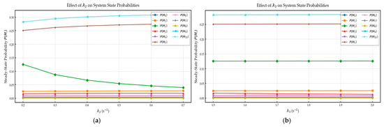
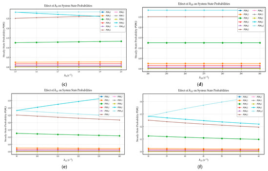
Figure 4.
The stable probability of each state under variations of different transition rates: (a) λ2—data preprocessing rate; (b) λ3—data entering the warning system rate; (c) λ9—system judged as no-warning rate; (d) λ10—red warning handling rate; (e) λ11—orange warning handling rate; (f) λ12—warning information review rate.
The simulation results reveal that different transition rates exert markedly distinct effects on the steady-state probability distribution. Among them, λ2, λ11, and λ9 are identified as the most sensitive parameters influencing system performance. As λ2 (data preprocessing rate) increases, the steady-state probability of intermediate backlog states decreases significantly. This indicates smoother data flow and reduced congestion within the simulated framework, suggesting that enhancing preprocessing efficiency can effectively mitigate potential delays in the model. In contrast, variations in λ11 (orange-alert handling rate) induce substantial fluctuations across several critical states, signifying that this stage represents a major operational bottleneck under the simulated conditions. A lower λ11 tends to cause task accumulation and alert delays, ultimately reducing system throughput. Meanwhile, λ9 (no-alert decision rate) exhibits relatively moderate changes but plays a stabilizing role by balancing the probabilities between the alert and non-alert branches, maintaining a more even distribution of processing resources. Overall, these three rates form a core sensitivity region within the model, providing insights into the internal dynamic behavior of the intelligent traffic warning system under varying transition conditions.
Based on the analysis, optimization should focus on the processes associated with λ2, λ11, and λ9. Enhancing λ2 can be achieved by improving data preprocessing efficiency through algorithmic parallelism and lightweight feature extraction to reduce system delay. For λ11, which represents the orange-alert handling stage, implementing priority-based scheduling and adaptive resource allocation could alleviate bottlenecks in alert processing. Regarding λ9, introducing an adaptive thresholding mechanism may help maintain system balance between alert and non-alert branches. These strategies collectively aim to enhance overall responsiveness and coordination efficiency. It should be noted, however, that these proposed improvements are not implemented or tested within the current SPN model. They are presented as conceptual directions for future work, where integrating data-driven rate adjustment and real-time adaptation mechanisms will be essential to transform the present static framework into a dynamic, self-optimizing intelligent traffic warning system.
5. Conclusions
This study constructs an evolutionary model of an intelligent traffic crisis early-warning system based on Stochastic Petri Nets (SPNs), providing an in-depth investigation of the interactions among multiple performance indicators within the system. Leveraging the theoretical foundations of SPNs, the research achieves significant progress in reliability modeling for fault-tolerant systems. The system’s operational states are elucidated in detail through analyses of average token counts and by observing the evolution of P(Mi) as the transition rates λi are varied. By exploiting the isomorphic properties between SPNs and Markov processes, the study further computes the steady-state probabilities of the intelligent traffic early-warning system, offering theoretical support for improving system efficiency.
While the proposed SPN-based modeling framework provides a structured and quantitative approach to analyze intelligent traffic early-warning systems, several limitations should be acknowledged. First, the model assumes that transition rates and initial conditions are well-defined and static, which may not fully capture the dynamic variability of real-world traffic flows. Second, the model primarily considers isolated intersections or limited network segments, and scaling it to larger urban networks may encounter state-space explosion or computational complexity. Third, extreme traffic conditions, unexpected driver behaviors, and sensor inaccuracies are not explicitly represented, which may affect the accuracy of system predictions.
In terms of real-world applicability, the model offers valuable insights for traffic management decision-making and early-warning system optimization, but its deployment requires integration with real-time traffic data and adaptive control strategies. Future work should focus on extending the SPN framework to handle heterogeneous traffic data, incorporate real-time feedback, and validate the model through field experiments to enhance its practical relevance.
Future research should focus on constructing multi-scenario, multi-level models of intelligent traffic systems, further exploring dynamic evolution and optimization methods under real-time data-driven conditions. In addition, integrating artificial intelligence and big data analytics can enhance the application of SPNs in intelligent traffic systems, improving both response speed and early-warning capability. Through continuous refinement and expansion, the proposed model will better equip intelligent traffic early-warning systems to cope with complex and rapidly changing traffic environments, providing robust support for the development of smart cities.
Author Contributions
Conceptualization, S.C.; Methodology, S.C. and F.N.; Software, S.C. and J.L.; Validation, S.C. and J.L.; Formal analysis, S.C.; Investigation, R.F. and Y.D.; Data curation, J.L.; Writing—original draft, S.C.; Writing—review and editing, F.N.; Visualization, S.C.; Supervision, F.N.; Project administration, F.N.; Funding acquisition, F.N. All authors have read and agreed to the published version of the manuscript.
Funding
National Natural Science Foundation of China (12371508); Ministry of Education Industry-University Cooperation Collaborative Education Project (241103760141654); Shanghai “College Students Innovation and Entrepreneurship Training Program” funded project (SH2025085, XJ2025167).
Data Availability Statement
The original contributions presented in this study are included in the article. Further inquiries can be directed to the corresponding author.
Conflicts of Interest
The authors declare no conflicts of interest.
References
- Li, Y. Research on the Risk Early Warning Mechanism of University Crisis Events. Forum Res. Innov. Manag. 2024, 2, 79–81. [Google Scholar] [CrossRef]
- Bhandari, A.; Pal, N.R. Can edges help convolution neural networks in emotion recognition? Neurocomputing 2021, 433, 162–168. [Google Scholar] [CrossRef]
- Li, J.; Shen, S.; Sun, X.; Xing, X. Identification and classification of risk paths in the context of cross-border flow of important data. Chin. J. Manag. Sci. 2021, 29, 90–99. [Google Scholar] [CrossRef]
- Masood, M.A.; Abbasi, R.A. Using graph embedding and machine learning to identify rebels on twitter. J. Inf. 2021, 15, 101–121. [Google Scholar] [CrossRef]
- Wu, X.; Wang, L.; Chen, H.; Zhang, L.; Zhang, K. Design and implementation of IoT-based subway structural health monitoring system based on BIM technology. Tunn. Constr. 2020, 40, 905. [Google Scholar]
- He, G.; Luo, X.; Zhang, H.; You, Q. Metro tunnel safety warning and forecasting technology based on the combination of BIM and GIS. Urban Rail Transit Res. 2019, 22, 161–164. [Google Scholar] [CrossRef]
- Zhang, J.; Liang, S.; Wei, C.; Liu, Y.; Chen, H. Ballastless track temperature monitoring and early warning system based on meteorological data. China Railway 2019, 41, 26–31. [Google Scholar] [CrossRef]
- Quan, X.; Zuo, G. NIMBY conflict evolution process model and scenario simulation analysis based on stochastic Petri nets: A case study of waste incineration power plants. Oper. Res. Manag. 2022, 31, 135–141. [Google Scholar] [CrossRef]
- Xu, N.; Tang, X. Research on 5W extraction of social risk events based on Baidu hot search news words. Syst. Eng.-Theory Pract. 2020, 40, 334–342. [Google Scholar]
- Yang, X.; Zheng, S.; Jin, Z.; Xiong, S. Research on the evaluation index system of network public opinion warning based on information ecology theory. Intell. Theory Pract. 2021, 44, 143–148. [Google Scholar] [CrossRef]
- Huang, W.; Huang, J.; Li, Y. Research on the early warning indicator system of cyber terrorist incidents. Intell. Mag. 2017, 36, 41–46. [Google Scholar]
- Tian, S.; Wang, C.; Yang, W. Research on early warning mechanism of network public opinion crisis of emergency events based on ANP and random Petri nets. Chin. J. Manag. Sci. 2023, 31, 215–224. [Google Scholar] [CrossRef]
- Huang, J.; Fu, P.; Xu, Y. Modeling of multi-department collaborative agricultural drought emergency response process based on stochastic Petri nets: A case study of Bayannur City, Inner Mongolia. J. Syst. Manag. 2021, 30, 1142–1151. [Google Scholar] [CrossRef]
- Zhang, Y.; Liang, Y.; Yin, M.; Quan, H.; Wang, T.; Jia, W. Survey on the methods of computation offloading in mobile edge computing. Chin. J. Comput. 2021, 44, 2406–2430. [Google Scholar]
- Chen, L.; Dong, J.D.; Pan, K.; Wang, Z. Survey of computation offloading strategies under cloud-edge-end and D2D edge architectures. Comput. Eng. Appl. 2023, 59, 55–67. [Google Scholar] [CrossRef]
- Lin, C.; Wang, Y.; Yang, Y.; Qu, Y. Research on network reliability analysis method based on stochastic Petri nets. J. Electron. 2006, 34, 322–332. [Google Scholar]
- Zhong, X.; Ni, F.; Liu, J.; Zhong, D.; Yin, X.; Zhao, R. Scenario-oriented business architecture modeling method based on ROADS. J. Univ. Shanghai Sci. Technol. 2023, 45, 415–424. [Google Scholar] [CrossRef]
- Huang, F.; Ni, F.; Liu, J.; Wang, X.; Gu, T.; Wu, X. Executable modeling method based on ROAD-CPN business architecture. J. Univ. Shanghai Sci. Technol. 2023, 45, 534–542. [Google Scholar] [CrossRef]
- Yan, Z.; Liu, W.; Du, Y. Modeling and analysis of subway emergency decision-making based on logical game probabilistic Petri net. J. Syst. Simul. 2023, 35, 1602–1618. [Google Scholar] [CrossRef]
- Li, J.; Li, Q.; Yang, L. Dynamic random flow Petri net modeling and analysis of urban road traffic system. Transp. Syst. Eng. Inf. 2010, 10, 134–139. [Google Scholar] [CrossRef]
- Huang, F.; Ni, F.; Liu, J.; Tao, M.; Zhou, Y.; Li, Y. Data flow modeling and verification of complex BPMN collaboration model based on HCPN. Comput. Integr. Manuf. Syst. 2024, 30, 1754–1769. [Google Scholar] [CrossRef]
- Sun, Q.; Guo, X.; Ma, F. Modeling and simulation of intercity passenger travel service process based on Petri net. J. Syst. Simul. 2019, 31, 189–198. [Google Scholar] [CrossRef]
- Xiao, J.; Zhang, Z.; Terzi, S.; Tao, F.; Anwer, N.; Eynard, B. Multi-scenario digital twin-driven human-robot collaboration multi-task disassembly process planning based on dynamic time petri-net and heterogeneous multi-agent double deep Q-learning network. J. Manuf. Syst. 2025, 83, 284–305. [Google Scholar] [CrossRef]
- Xiao, J.; Zhang, Z.; Terzi, S.; Anwer, N.; Eynard, B. Dynamic task allocations with Q-learning based particle swarm optimization for human-robot collaboration disassembly of electric vehicle battery recycling. Comput. Ind. Eng. 2025, 204, 111133. [Google Scholar] [CrossRef]
- Jafari, S.; Shahbazi, Z.; Byun, Y.-C. Traffic control prediction design based on fuzzy logic and lyapunov approaches to improve the performance of road intersection. Processes 2021, 9, 2205. [Google Scholar] [CrossRef]
- Tunc, I.; Yesilyurt, A.Y.; Soylemez, M.T. Different fuzzy logic control strategies for traffic signal timing control with state inputs. IFAC-PapersOnLine 2021, 54, 265–270. [Google Scholar] [CrossRef]
- Gao, C.; Lan, X.; Li, N.; Yuan, Y.; Ding, J.; Zhou, Z.; Xu, F.; Li, Y. Large language models empowered agent-based modeling and simulation: A survey and perspectives. Humanit. Soc. Sci. Commun. 2024, 11, 1259. [Google Scholar] [CrossRef]
- Bastarianto, F.F.; Hancock, T.O.; Choudhury, C.F.; Manley, E. Agent-based models in urban transportation: Review, challenges, and opportunities. Eur. Transp. Res. Rev. 2023, 15, 19. [Google Scholar] [CrossRef]
- GA/T 928–2011; Specification for Striated Toolmark Examination of Forensic. Standardization Administration of China (SAC): Beijing, China, 2011.
- GA/T 1400–2017; Video and Image Information Application System For Public Security—Part 1: General Technical Requirements. Standardization Administration of China (SAC): Beijing, China, 2017.
- GA/T 1301–2016; Rules for Determining the Cause of a Fire. Standardization Administration of China (SAC): Beijing, China, 2016.


Disclaimer/Publisher’s Note: The statements, opinions and data contained in all publications are solely those of the individual author(s) and contributor(s) and not of MDPI and/or the editor(s). MDPI and/or the editor(s) disclaim responsibility for any injury to people or property resulting from any ideas, methods, instructions or products referred to in the content. |
© 2025 by the authors. Licensee MDPI, Basel, Switzerland. This article is an open access article distributed under the terms and conditions of the Creative Commons Attribution (CC BY) license (https://creativecommons.org/licenses/by/4.0/).