Stochastic Free-Vibration Analysis of Horizontal Single-Axis Solar Tracking Brackets

Abstract

As a large-scale flexible structure, the free-vibration characteristics of a horizontal single-axis solar tracking bracket (HSSTB) hold significance for its dynamic optimization design. However, due to material fabrication, construction processes, and harsh field service environments, structural parameters such as the elastic modulus inevitably exhibit uncertainty, leading to discrepancies between actual free-vibration characteristics and design values. This study considers the randomness of the steel elastic modulus and conducts a global sensitivity analysis of a real-life five-column HSSTB. First, the Kriging method is employed to build a surrogate model to describe the natural frequencies of the HSSTB and its stochastic parameters, which enables efficient evaluation of the statistical characteristics of the HSSTB’s natural frequencies. Further, the Sobol indices are utilized to quantify the influence of parameter randomness on the natural frequencies. The results indicate that the mean values of the first five natural frequencies are slightly lower than the design values. The first, fourth, and fifth natural frequencies of the five-column HSSTB are predominantly influenced by the middle three columns, while the second and third natural frequencies are more susceptible to the two edge columns.

1. Introduction

Under the impetus of the global energy structure transformation and the sustainable development strategy, solar energy, as a clean and renewable energy source, has been increasingly widely applied. Photovoltaic power generation, as one of the main forms of solar energy utilization, has developed rapidly in recent years [1,2,3]. The horizontal single-axis solar tracking bracket (HSSTB) (Figure 1) has become one of the mainstream choices for large-scale photovoltaic power stations due to its ability to effectively enhance the utilization rate of solar energy.

HSSTBs typically feature large spans, low rigidity, and small damping. They are often constructed in areas prone to wind and sand erosion, such as plains and deserts. Therefore, vibration under wind load is a key factor affecting the dynamic response of the structure [4]. A thorough understanding of the free-vibration characteristics of the structure is the basis for studying the wind-induced vibration response.

In reality, due to uncertainties in material production and construction processes, coupled with the fact that the service environment of photovoltaic brackets is usually harsh, often subject to wind and sand erosion and rain corrosion, as well as the influence of extreme temperature changes, these factors jointly lead to a significant difference between the free-vibration characteristics of the bracket system and the design values. Therefore, modeling from the perspective of uncertainty would be more reasonable, and the uncertainty quantification of the free-vibration characteristics is of great significance for the dynamic reliability analysis and optimization design of structures.

At present, the dynamic response characteristics of HSSTBs are mostly concentrated on the wind-vibration response and are usually based on deterministic models [5,6,7], which implies that the model parameters of the HSSTB are consistent with the design values after construction and will not change during service. For instance, Davenport [8] proposed the gust load factor method to employ probability theory in the study of structural wind response, laying the foundation for the development of structural wind engineering. Liu et al. [9] conducted wind tunnel tests based on an elastic test model to study the wind-induced response and critical wind speed of the support structure of flexible photovoltaic modules with a span of 33 m, and they investigated the effects of three stabilizing cables on improving the critical wind speed of the support structure of flexible photovoltaic modules in detail. Chen et al. [10] reviewed the latest research on the aerodynamic characteristics and wind-induced response of flexible photovoltaic systems, conducted relevant studies using physical or numerical simulation tools, and considered the influence of a series of control parameters (such as pitch ratio, angle of attack, tilt angle, and position).

All the above studies have modeled and analyzed the wind-induced vibration response characteristics of photovoltaic brackets from a deterministic perspective. Currently, there are few studies on the free-vibration characteristics and parameter sensitivity of HSSTBs from an uncertainty perspective. Introducing the uncertainty of material parameters can more reasonably reflect the influence of complex field service environments on the natural vibration characteristics of solar tracking brackets. On this basis, through global sensitivity index analysis based on random samples, the key parameters affecting the free-vibration characteristics can be identified, thereby providing an important reference for the dynamic reliability and optimized design of HSSTBs [11].

For the free-vibration analysis of random structures, various methods have been developed, including the Monte Carlo simulation method (MCS method) [12], perturbation method [13,14], polynomial chaos expansion method (PC method) [15], and homotopy finite element method [16,17,18]. The MCS method requires a large number of samples to obtain convergent statistical results. For complex engineering structures, the calculation process of the MCS method is extremely time-consuming. The perturbation method is only applicable to situations where the variability in structural parameters is relatively small or there is a linear relationship between the random inputs and output. When the dimension of the random inputs is relatively high, the PC method may encounter the “curse of dimensionality”. Recent advances further include machine-learning surrogates for stochastic free-vibration of graded bars [19], closed-form probabilistic treatments of eigenpairs for stochastic symmetric systems via probability transformation methods [20], efficient stochastic modal decomposition strategies for static/dynamic problems [21], and even quantum-computing-assisted eigenvalue analysis for stochastic structures [22]. Against this background and considering the scale and modeling needs of the present HSSTB problem, we adopt a Kriging surrogate to balance accuracy and efficiency for uncertainty quantification and global sensitivity analysis of the random free-vibration characteristics.

The magnitude of the influence of each random parameter on the free-vibration characteristics of the structure can be achieved through sensitivity analysis. Sensitivity analysis includes local sensitivity analysis and global sensitivity analysis. The former is generally used to describe the sensitivity of parameters near the mean or design value, essentially being the slope at a certain point [23,24]. The latter can reflect the influence of the entire sample space variation on the response uncertainty. Various global sensitivity indices have been proposed, including derivatives-based [25], variance decomposition [26], moment-independent [27], distribution-based [28], and Frechet-derivative-based [29,30], etc. Among them, the variance-decomposition-based global sensitivity index, which is known as the Sobol index, has been widely applied in practical engineering because it can reflect the contribution of the variance of the input variable to the variance of the output response [31,32,33].

Although the Kriging method and Sobol sensitivity analysis are established techniques, their combined application to quantify the uncertainty in free-vibration characteristics of a real-life HSSTB is novel. This study fills a gap in the literature by moving beyond deterministic models and providing a practical framework for identifying which structural components most significantly influence the natural frequencies of these large, flexible systems. This is crucial for targeted dynamic optimization and reliability assessment under parameter uncertainties arising from manufacturing and harsh environmental conditions.

Based on the above background, this paper takes a five-column HSSTB in Gansu Province, China, as an example. As the material variability is often the dominant contributor to stiffness uncertainty in steel columns, the elastic modulus is chosen as the primary uncertainty parameter due to its significant susceptibility to material and environmental variations. Considering the randomness of the elastic modulus of the steel columns, a fine finite element model of the HSSTB is first established by using ANSYS. Then, the random free-vibration characteristics of the structure are studied through the Kriging method. Finally, a global sensitivity analysis of the structural random parameters is conducted in combination with the Sobol index to explore the main influencing factors. The analysis results can provide a reference for the dynamic response analysis and optimal design of the bracket system.

2. Finite Element Model of the Horizontal Single-Axis Solar Tracking Bracket

2.1. Project Overview

The HSSTB studied is the 40 MW photovoltaic power generation project of China Resources Power located in Sangke Grassland, Amuqihu Town, Gansu Province. The size of each photovoltaic panel component is 2278 × 1134 × 35 mm, with a power of 545 Wp. The system is single-axis drive, consisting of 26 components in a string, 52 components per axis, a single set power of 28.34 kW, and five piles per row. The model is generally divided into three parts: a concrete cylinder at the bottom, a steel column, and a photovoltaic panel at the top. The columns and photovoltaic panels are connected through the transverse main beams, diagonal braces, and purlins. The materials of the connection parts are all steel, and the material properties of these components are shown in

Table 1. Material parameters for each component.

	Element Type	Elastic Modulus (Pa)	Poisson’s Ratio	Density (kg·m−3)
Concrete	BEAM188	3.6 × 1010	0.167	2700
Section steel	BEAM188	20.6 × 1010	0.25	7850
Photovoltaic panel	SHELL63	8.8 × 1010	0.15	2560

. The equivalent properties for photovoltaic panels represent a composite of glass and aluminum frame components. All connections between purlins and panels were modeled as rigid, while additional masses from cabling and equipment are small (estimated <2% of the total mass) and do not significantly affect the fundamental modal characteristics. There are four different cross-sectional forms for the steel components, namely, I-beam columns with the model H203 × 102 × 5.8 × 6.8, square steel main beams with the model 140 × 140 × 2.5, Z-shaped steel purlins with the model 30 × 80 × 79 × 1.5, and C-shaped steel diagonal braces with the model 32 × 38 × 2.

2.2. Finite Element Model

The actual structure and the corresponding finite element model are shown in Figure 2.

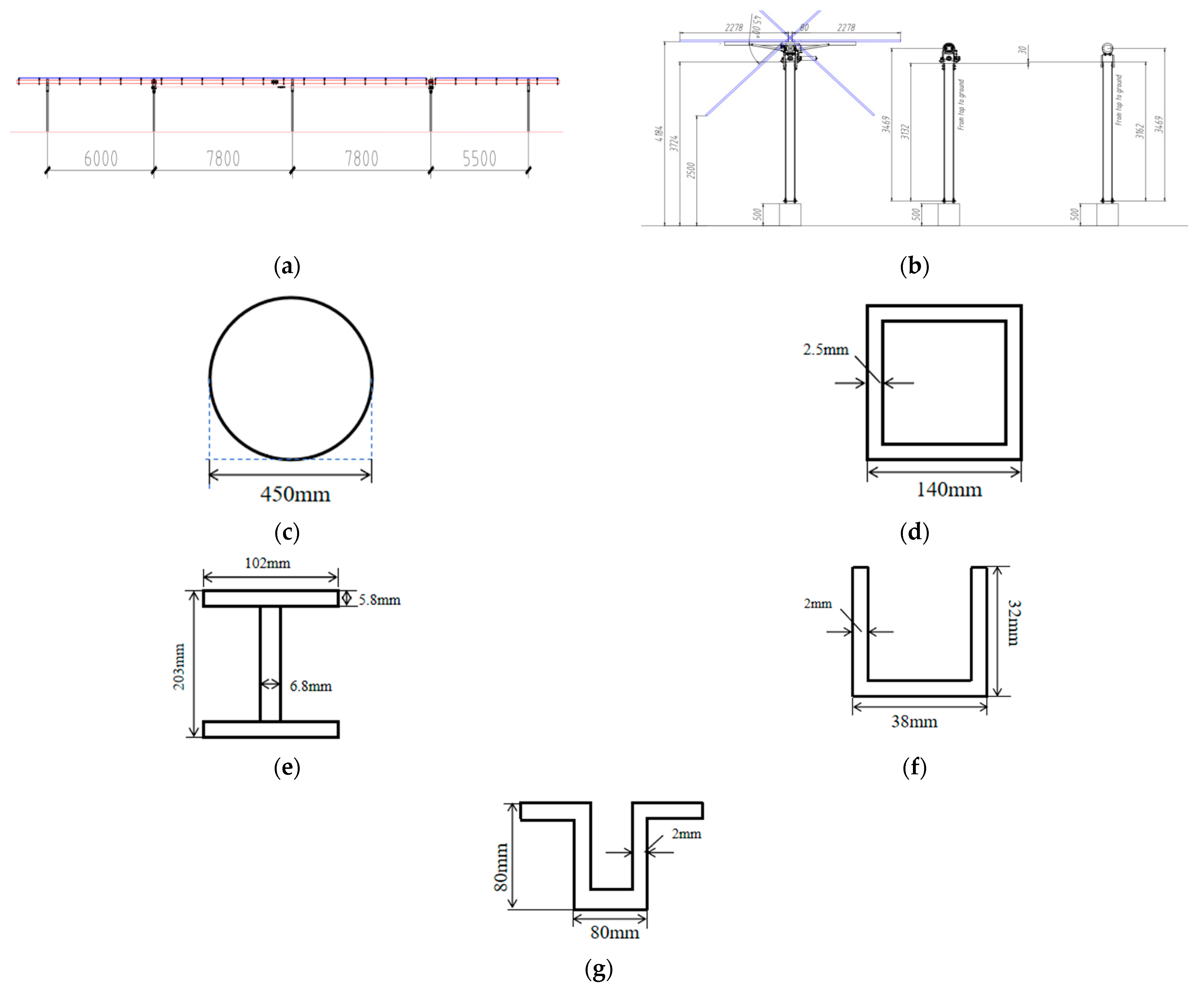
The photovoltaic panels are simulated using SHELL63 elements, while the steel section columns, main beams, purlins, and diagonal braces are simulated using BEAM188 elements. In addition, the foundation concrete pile is represented by BEAM188 for modeling the cylindrical pile in a beam formulation to reduce model complexity while preserving bending and axial stiffness. The cross-sectional length, width, and thickness of these components are shown in Figure 3a–g. The finite element model of this five-column HSSTB consists of a total of 453 elements and 2490 degrees of freedom.

2.3. Experimental Validation After Reinforcement

To verify the adequacy of the finite element (FE) modeling assumptions described in Section 2.2, an on-site ambient-vibration test was conducted after reinforcement of the support system (as shown in Figure 4). In the reinforced configuration, the lower 2.5 m of each support column was jacketed with channel-steel sections to enhance local stiffness. The experimental measurements therefore correspond to the reinforced structure, matching the configuration used in the corresponding FE analyses.

In the actual facility, a previously observed structural failure initiated at the columns and led to system collapse, while the upper photovoltaic (PV) panels and auxiliary components remained intact. Because the present study focuses on how column parameter variability affects the free-vibration characteristics, the test boundary conditions were arranged to isolate column behavior and to be consistent with the FE idealization: the drive-column motor was switched off during testing to eliminate actuator-induced rotations; the top transverse beam was mechanically restrained against rotation (limited/locked) to avoid tracker motion; and in the FE model, the five columns are modeled as rigidly connected (fully fixed) to the top beam, i.e., no relative rotation between each column head and the beam is permitted.

A set of accelerometers were mounted on the structure, and ambient excitation (environmental/operational loads) was used to excite the system. Data were acquired in multiple batches, with each batch lasting 10 min to ensure repeatability and improve the signal-to-noise ratio. The measured acceleration responses were processed in the frequency domain to identify the first three natural frequencies of the reinforced system under the restrained-beam condition described above.

Table 2. Comparison of measured and FE-predicted natural frequencies of the reinforced five-column HSSTB.

Mode	Measured (Hz)	FE (ANSYS) (Hz)	Relative Error vs. Measurement (%)
1	0.340	0.328	9
2	0.348	0.354	7
3	0.355	0.374	5

reports the experimentally measured first three natural frequencies together with the ANSYS FE predictions for the same reinforced configuration. Across the first three modes, the relative discrepancies between the measured and computed frequencies lie within approximately 5–10%. Considering environmental excitation, boundary-condition idealizations, and measurement noise, this level of agreement indicates that the developed FE model provides a reasonable and reliable baseline for the subsequent stochastic analysis and Sobol sensitivity assessment. The alignment between the imposed experimental restraints and the FE constraints (columns fully fixed to the top beam) ensures that the comparison is physically meaningful and that the reported differences are primarily attributable to the inherent variability in column properties rather than uncontrolled rotational freedoms of the tracker assembly.

The modal analysis shows that the first five vibration modes of the solar bracket structure are predominantly translational in the Y-direction (lateral), with the rotational energy content remaining low (13–19% range) across all modes. This demonstrates that torsional components are negligible in the fundamental modes, primarily due to the structure’s high in-plane torsional stiffness and uniform mass distribution. The vibration characteristics are dominated by column bending behavior, with significant torsional modes expected to appear only in higher frequency ranges beyond the first five modes.

3. Stochastic Free-Vibration Equation for the HSSTB

3.1. Establishment of the Stochastic Free-Vibration Equation

The free-vibration equation of a deterministic structure is as follows:

$${\mathit{K}}_{\left(N\times N\right)}{\mathsf{\Phi }}_{\left(N\times N\right)}={\mathsf{\Lambda }}_{\left(N\times N\right)}{\mathit{M}}_{\left(N\times N\right)}{\mathsf{\Phi }}_{\left(N\times N\right)}$$

(1)

where N represents the degrees of freedom of the finite element model of the structure. K and M, respectively, represent the global stiffness matrix and mass matrix of the HSSTB. $\Lambda =\mathrm{diag}\left({\lambda }^{\left(1\right)}{\lambda }^{\left(2\right)}\dots {\lambda }^{\left(N\right)}\right)$ and $\mathsf{\Phi }=\mathrm{diag}\left({\mathit{\varphi }}^{\left(1\right)}{\mathit{\varphi }}^{\left(2\right)}\dots {\mathit{\varphi }}^{\left(N\right)}\right)$ are eigenvalues and eigenvectors, respectively. For the j-th eigenvalue and eigenvector, it satisfies the following equation

$${\mathit{K}}_{\left(N\times N\right)}{{\mathit{\varphi }}^{\left(j\right)}}_{\left(N\times 1\right)}={\lambda }^{\left(j\right)}{\mathit{M}}_{\left(N\times N\right)}{{\mathit{\varphi }}^{\left(j\right)}}_{\left(N\times 1\right)}$$

(2)

The eigenvectors ${\mathit{\varphi }}^{\left(j\right)}$ can be normalized through the mass matrix, which is ${\mathit{\varphi }}^{\left(j\right)T}\mathit{M}{\mathit{\varphi }}^{\left(j\right)}=1$.

Considering the randomness of the material (such as elastic modulus), the stiffness of the HSSTB can be expressed as $\mathit{K}\left(\xi \right)={\mathit{K}}_0+{\displaystyle \sum _{i=1}^n{\mathit{K}}_i}{\xi }_i$, where $\xi$ are random variables. Then, the free-vibration equation can be written as

$$\left({\mathit{K}}_{0\left(N\times N\right)}+{\displaystyle \sum _{i=1}^n{\mathit{K}}_{i\left(N\times N\right)}}{\xi }_i\right){{\mathit{\varphi }}^{\left(j\right)}}_{\left(N\times 1\right)}\left(\xi \right)={\lambda }^{\left(j\right)}\left(\xi \right){\mathit{M}}_{\left(N\times N\right)}{{\mathit{\varphi }}^{\left(j\right)}}_{\left(N\times 1\right)}\left(\xi \right)$$

(3)

Equation (3) is solved to obtain the j-th eigenvalue ${\lambda }^{\left(j\right)}\left(\xi \right)$ and eigenvector ${\mathit{\varphi }}^{\left(j\right)}\left(\xi \right)$. ${\mathbf{\omega }}^{\left(j\right)}\left(\xi \right)=\sqrt{{\lambda }^{\left(j\right)}\left(\xi \right)}$ represents the j-th natural frequency of the HSSTB, and ${\mathit{\varphi }}^{\left(j\right)}\left(\xi \right)$ corresponds to the j-th mode shape of the HSSTB.

3.2. Solution of the Free-Vibration Equation Based on the Kriging Method

Firstly, suppose the natural frequency $\mathrm{\omega }\left(\xi \right)$ is a Gaussian process, which can be expressed as

$$\mathbf{\omega }\left(\xi \right)=h{\left(\xi \right)}^T\beta +{\rm Z}\left(\xi \right)$$

(4)

In Equation (4), $\xi$ is the input random variables; $h\left(\xi \right)$ is a basis function vector which is a zero-order polynomial; $\beta$ is the regression coefficient vector; and ${\rm Z}\left(\xi \right)$ is a Gaussian random process with a mean of zero, and its covariance function is

$$\mathrm{Cov}\left. [{\rm Z}\left({\xi }_i\right),{\rm Z}\left({\xi }_j\right)\right]={\sigma }^{2}R\left({\xi }_i,{\xi }_j\right)$$

(5)

where ${\sigma }^2$ is the variance of the process, and $\mathrm{R}\left({\xi }_i,{\xi }_j\right)$ is the correlation function, which uses a Gaussian (squared-exponential) kernel with anisotropic length scales. The hyperparameters, the process variance, and a small nugget are estimated by maximum likelihood estimation (MLE) with bound-constrained gradient-based optimization.

To establish the Kriging model, G sample points, $\xi =\left. [{\xi }^{(1)},{\xi }^{(2)},\cdots ,{\xi }^{(G)}\right]$, are selected according to the distributions of the input variables through Latin hypercube sampling (LHS), and their corresponding natural frequencies $\omega =\left. [{\omega }^{(1)},{\omega }^{(2)},\cdots ,{\omega }^{(G)}\right]$ are calculated through Equation (1). Then, the regression coefficients are computed through the generalized least square method as follows

$$\beta ={\left({\mathbf{H}}^T{\mathbf{R}}^{-1}\mathbf{H}\right)}^{-1}{\mathbf{H}}^T{\mathbf{R}}^{-1}\mathbf{\omega }$$

(6)

where the matrix R has the following form

$$\mathbf{R}=\left. [\begin{array}{cccc}R\left({\xi }^{(1)},{\xi }^{(1)}\right)& R\left({\xi }^{(1)},{\xi }^{(2)}\right)& \dots & R\left({\xi }^{(1)},{\xi }^{(n)}\right)\\ R\left({\xi }^{(2)},{\xi }^{(1)}\right)& R\left({\xi }^{(2)},{\xi }^{(2)}\right)& \dots & R\left({\xi }^{(2)},{\xi }^{(n)}\right)\\ ⋮& ⋮& \ddots & ⋮\\ R\left({\xi }^{(n)},{\xi }^{(1)}\right)& R\left({\xi }^{(n)},{\xi }^{(2)}\right)& \dots & R\left({\xi }^{(n)},{\xi }^{(n)}\right)\end{array}\right]$$

(7)

The regression matrix H is expressed as

$$\mathbf{H}=\left. [\begin{array}{c}h{\left({\xi }^{(1)}\right)}^T\\ h{\left({\xi }^{(2)}\right)}^T\\ ⋮\\ h{\left({\xi }^{(n)}\right)}^T\end{array}\right]$$

(8)

The process variance ${\sigma }^2$ is estimated as

$${\sigma }^2={\displaystyle \frac{1}{n}}{\left(\mathbf{\omega }-\mathbf{H}\beta \right)}^T{\mathbf{R}}^{-1}\left(\mathbf{\omega }-\mathbf{H}\beta \right)$$

(9)

For a new input random variable sample ${\xi }^{*}$, the predicted value of its natural frequency is $\hat{\mathbf{\omega }}\left({\xi }^{*}\right)$, which can be computed as

$$\hat{\mathbf{\omega }}\left({\xi }^{*}\right)=\mathbf{h}{\left({\xi }^{*}\right)}^T\beta +\mathbf{r}{\left({\xi }^{*}\right)}^T{\mathbf{R}}^{-1}\left(\mathbf{\omega }-\mathbf{H}\beta \right)$$

(10)

where $\mathbf{r}\left({\xi }^{*}\right)$ is the correlation vector between the new sample point ${\xi }^{*}$ and the known sample points

$$\mathbf{r}\left({\mathbf{X}}^{*}\right)=\left. [\begin{array}{c}R\left({\xi }^{*},{\xi }^{1)}\right)\\ R\left({\xi }^{*},{\xi }^{(2)}\right)\\ ⋮\\ R\left({\xi }^{*},{\xi }^{(n)}\right)\end{array}\right]$$

(11)

Through the Kriging surrogate model Equation (10), a sufficient number of natural frequency samples can be generated efficiently, and then statistical analysis of the natural frequencies and global sensitivity analysis of the input variables can be conducted.

3.3. Global Sensitivity Analysis of Natural Frequencies

Let a single-output random system be described by model $y=g(\xi )$, where y is a scalar random output and $\xi$ is the n random inputs of the system. According to Sobol decomposition, $y=g(\xi )$ can be expressed as follows:

$$y(\xi )=g_0+{\displaystyle \sum _{i=1}^n{g}_i({\xi }_i)+}{\displaystyle \sum _{i=1}^{n-1}{\displaystyle \sum _{j=i+1}^n{g}_{i,j}({\xi }_i,{\xi }_j)}}+\cdots +g_{1,2,\dots ,n}({\xi }_1,\cdots ,{\xi }_n)$$

(12)

$$\begin{array}{l}{g}_0=E(y)\\ g_i({\xi }_i)=E(y|{\xi }_i)-g_0\\ g_{i,j}({\xi }_i,{\xi }_j)=E(y|{\xi }_i,{\xi }_j)-g_i-g_j-g_0\\ \dots \end{array}$$

(13)

$E(y|{\xi }_i)$ represents the expected conditional probability of y when ${\xi }_i$ is fixed, $E(y|{\xi }_i,{\xi }_j)$ represents the expected conditional probability of y when both ${\xi }_i$ and ${\xi }_j$ are fixed, and so on. Taking the variance on both sides of Equation (12) gives:

$$V\left(y(\xi )\right)={\displaystyle \sum _{i=1}^{n}V\left(g_i({\xi }_i)\right)+}{\displaystyle \sum _{i=1}^{n-1}{\displaystyle \sum _{j=i+1}^{n}V\left(g_{i,j}({\xi }_i,{\xi }_j)\right)}}+\cdots +V\left(g_{1,2,\dots ,n}({\xi }_1,\cdots ,{\xi }_n)\right)$$

(14)

Substituting Equation (13) into Equation (14) and dividing both sides of Equation (14) by $V\left(y(\xi )\right)$, we obtain:

$$1={\displaystyle \sum _{i=1}^n{S}_i}+{\displaystyle \sum _{i=1}^{n-1}{\displaystyle \sum _{j=i+1}^n{S}_{i,j}}}+\cdots +S_{1,2,\dots ,n}$$

(15)

where $S_{i_1,i_2,\dots ,i_r}={\displaystyle \frac{V\left(g_{i_1,i_2,\dots ,i_r}({\xi }_{i_1},{\xi }_{i_2},\cdots ,{\xi }_{i_r})\right)}{V\left(y(\xi )\right)}}$ represents the contribution of the interaction of the r input variables $({\xi }_{i_1},{\xi }_{i_2},\dots ,{\xi }_{i_r})$ to the variance of the output y. The commonly used $S_i$ is called the main effect indicator, which can reflect the individual contribution of ${\xi }_i$ to the variance of the random output y.

The calculation process of the global sensitivity index $S_i$ of the natural frequency corresponding to the i-th random variable ${\xi }_i$ is as follows: First, generate two sets of sample matrices $A_{(G\times n)}$ and $B_{(G\times n)}$ with the number G for the n random variables. Replace the i-th column of $B_{(G\times n)}$ with the i-th column of $A_{(G\times n)}$ to generate the sample matrix $C_{(G\times n)}^i$. Calculate the natural frequency samples ${{\mathit{\omega }}^A}_{ (1\times G)}$ and ${{\mathit{\omega }}^{C^i}}_{ (1\times G)}$ corresponding to $A_{(G\times n)}$ and sample matrix $C_{(G\times n)}^i$, respectively, using Equation (10). Then, the calculation expression of $S_i$ as follows

$$S_i={\displaystyle \frac{\frac{1}{G}{\displaystyle \sum _{k=1}^G{\mathit{\omega }}^A}(k){\mathit{\omega }}^{C^i}(k)-{\left. [\frac{1}{G}{\displaystyle \sum _{k=1}^G{\mathit{\omega }}^A(k)}\right]}^2}{\frac{1}{G}{\displaystyle \sum _{k=1}^G{\mathit{\omega }}^A{(k)}^2}-{\left. [\frac{1}{G}{\displaystyle \sum _{k=1}^G{\mathit{\omega }}^A(k)}\right]}^2}}$$

(16)

4. Numerical Example

A global sensitivity analysis of the natural frequency of a five-column HSSTB in Gansu Province, China, is conducted. Firstly, a global sensitivity analysis of a photovoltaic steel column is carried out to investigate the influence of sample point selection and the variability in random variables on the results of the Kriging method, and the accuracy of the Kriging method is verified by the calculation results of the MCS method. Then, the Kriging method is used to conduct a global sensitivity analysis of the five-column HSSTB to study the influence of parameter randomness on the natural vibration characteristics of the system, so as to provide a reference for the dynamic optimization design of the structure.

4.1. Global Sensitivity Analysis of the Natural Vibration Characteristics of the Photovoltaic Steel Column

As shown in Figure 5a, a 3.5 m tall H-shaped steel photovoltaic steel column is fixed at the bottom and free at the top. To enhance the column’s stability during its service period, the lower 2 m height range is reinforced by wrapping it with channel steel. The geometric parameters of the column’s cross-section are presented in Figure 5b,c.

The finite element model of this column consists of 70 beam elements, each with a length of 0.05 m. The average elastic modulus E₀ of the steel is 20.6 × 10¹⁰ Pa, the moment of inertia of section AB of the reinforced part is 8.68 × 10⁻⁵ m⁴, and that of section BC is 6.92 × 10⁻⁵ m⁴. The randomness of the elastic modulus within a length range of 0.25 m along the column height direction is described by one random variable, expressed as $E_0\left(1+\delta \xi \right)$. Among them, $\delta$ is the parameter that controls the magnitude of the elastic modulus variability. Then, the elastic modulus of the AB segment contains eight random variables (ξ₁ to ξ₈), and the elastic modulus of the BC segment contains six random variables (ξ₉ to ξ₁₄). For ξ₁ to ξ₈, first, log-normal samples with a mean of 1 and standard deviation of 0.1 are generated. Then, the mean of 1 is subtracted from each sample to obtain random samples with a mean of 0 and standard deviation of 0.1. For ξ₉ to ξ₁₄, first, samples are generated from a Beta distribution with parameters α = 2 and β = 10. Then, the mean of 1/6 is subtracted from each sample to obtain random samples with a mean of 0 and standard deviation of 0.1. This processing ensures that when the steel modulus of elasticity is expressed as $E_0\left(1+\delta \xi \right)$, the sample mean of the steel modulus of elasticity equals the nominal design value E₀, and its coefficient of variation (CoV) is 0.1 $\delta$.

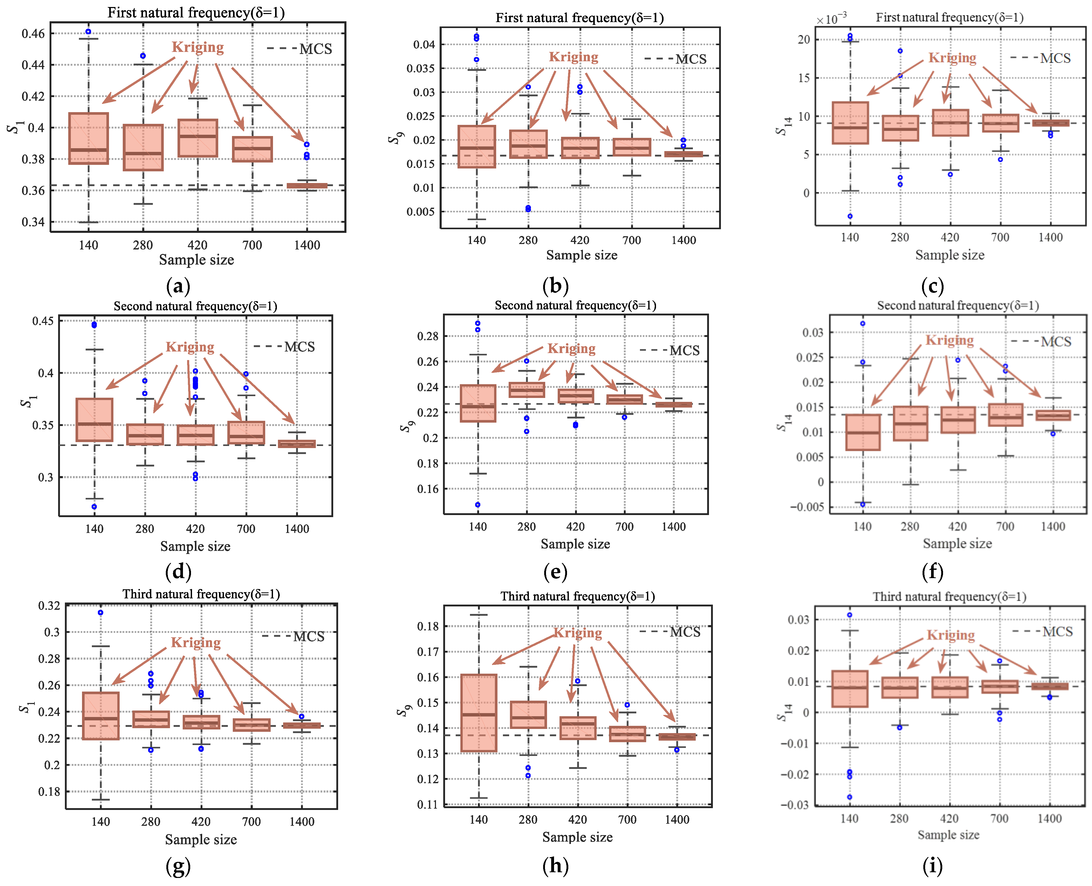
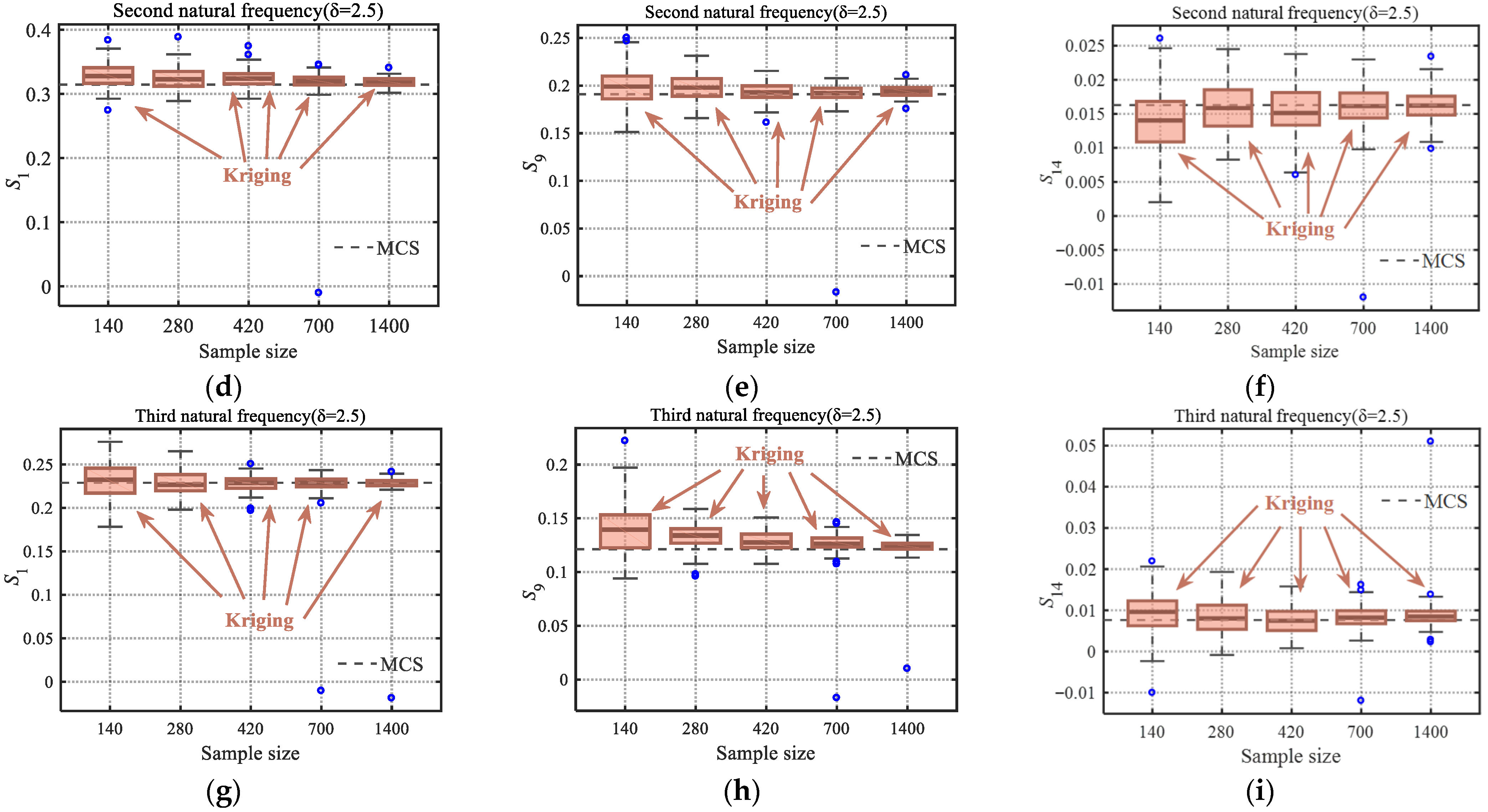
The two cases of $\delta$ = 1 and $\delta$ = 2.5 are discussed, corresponding to the CoV of the elastic modulus of steel being 0.1 (small variation) and 0.25 (moderate variation), respectively. Figure 6 and Figure 7, respectively, present the Sobol indices corresponding to the first three natural frequencies of the support column at the bottom (ξ₁), the variable section (ξ₉), and the top (ξ₁₄) of the column under two cases of small variation ($\delta$ = 1) and moderate variation ($\delta$ = 2.5) of the random variable, which are denoted as S₁, S₉, and S₁₄, respectively. The Kriging method establishes surrogate models using sample points that are 10, 20, 30, 50, and 100 times the number of random variables respectively, and conducts 100 repeated calculations. The MCS results based on 10,000 samples are taken as the reference solution.

As can be seen from Figure 6, when the variability in random variables is relatively small, as the sample size increases, the results of S₁, S₉, and S₁₄ calculated by the Kriging method gradually converge to those of the MCS method. Moreover, the more samples used, the smaller the variability in the calculation results, that is, the robustness is enhanced. When the variability in the random variable increases, as shown in Figure 7, when the same sample size is used to construct the surrogate model, the variability in the global sensitivity indices of the natural frequency calculated by the Kriging method will increase. However, regardless of whether the variation is small or large, when the Kriging method takes 1400 samples, the mean of all Sobol index results is very close to that of the MCS.

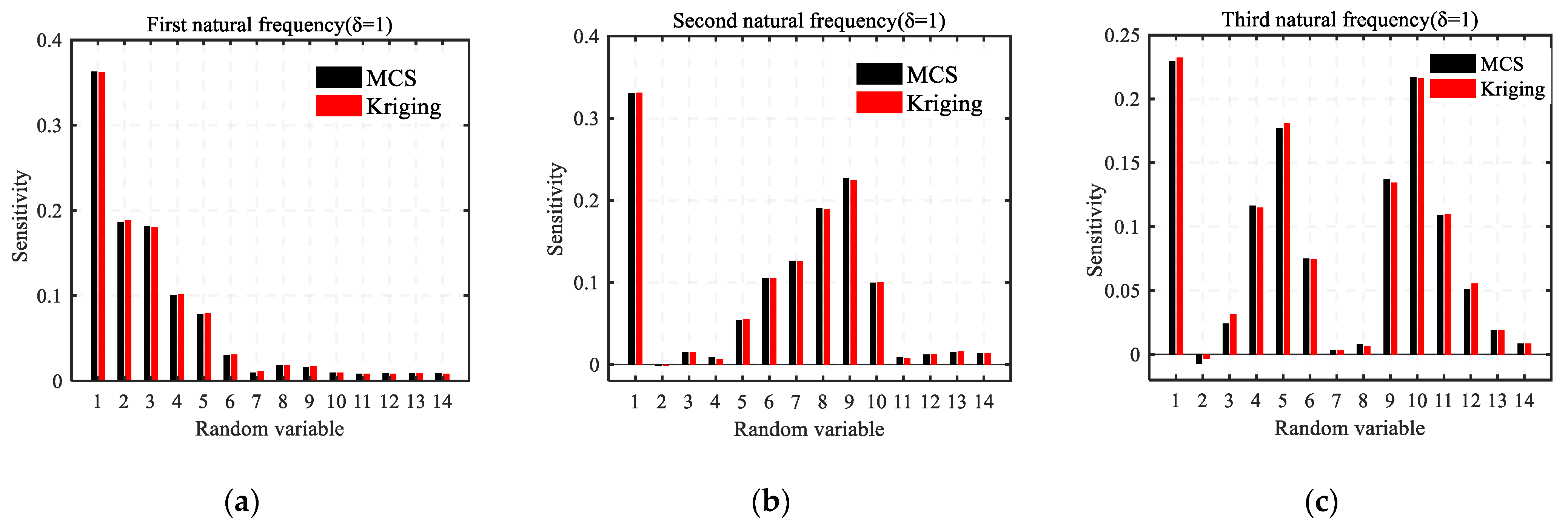
Figure 8 presents the Sobol indices of all random variables of the first three natural frequencies under small variation, where the Kriging method uses 1400 samples to establish a surrogate model. It can be seen that the main influencing factors of different natural frequencies are significantly different. The area with the greatest response to the first natural frequency is ξ₁ to ξ₃, which is concentrated in the reinforced part at the bottom of the column. The factors that have the greatest impact on the second natural frequency are ξ₁, ξ₈, and ξ₉, namely, the bottom of the column and the variable cross-section. The factors that have the greatest impact on the third natural frequency are ξ₁, ξ₅, and ξ₁₀. It is indicated that as the mode of the natural frequency increases, the major influencing factors gradually become more evenly distributed along the column height direction. However, the bottom of the column always has a key impact. This is because the constraint strength of the fixed section of the cantilever component will directly affect the natural vibration characteristics of the structure.

As can be seen from Figure 9, when the variability in random variables increases, the accuracy of the calculation results of the Kriging surrogate model constructed with the same samples will slightly decrease. However, it has almost no impact on the ranking of the importance of each parameter.

4.2. Global Sensitivity Analysis of Random Free-Vibration of the Five-Column HSSTB

4.2.1. Global Sensitivity Analysis of the Five-Column HSSTB Before Reinforcement

First, the free-vibration characteristics of the five-column HSSTB before reinforcement are studies, that is, the working condition described in Section 2.1. During the process of establishing the surrogate model by the Kriging method, the number of Latin hypercube samples is 1000. Suppose the elastic moduli of the five columns all follow a Beta distribution with a mean of 0 and a standard deviation of 0.1. There are five random variables, one per column, which represent column-wise spatially averaged elastic modulus uncertainties. Each column is discretized into 15 finite elements for structural resolution, but stochastic variation is applied as a single random variable per column. Because the five steel columns are distinct members with separate fabrication, handling, and installation histories. Assume that the elastic modulus of the column is expressed as $E_0\left(1+\xi \right)$, then coefficients of variability of the elastic modulus is 0.1. The material parameters of other components are considered deterministic.

Figure 10 shows an excellent one-to-one agreement between the Kriging predictions and the true results for the first natural frequency of the unreinforced five-column HSSTB, with R² = 0.99962. Data points cluster tightly around the y = x line with no visible bias across the frequency range, indicating very small residuals. This confirms that the surrogate is sufficiently accurate for subsequent stochastic sampling and Sobol’ sensitivity analysis.

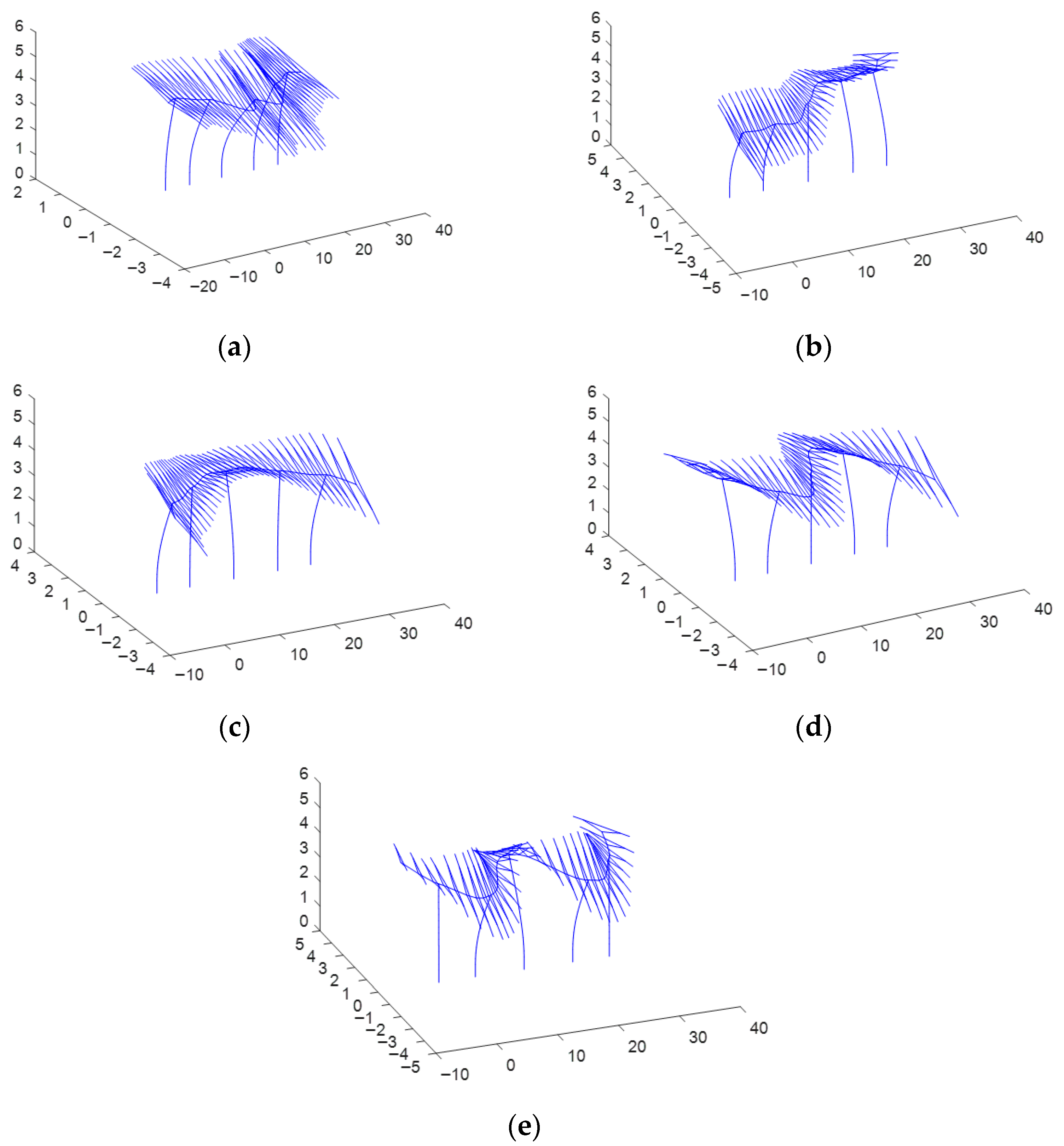
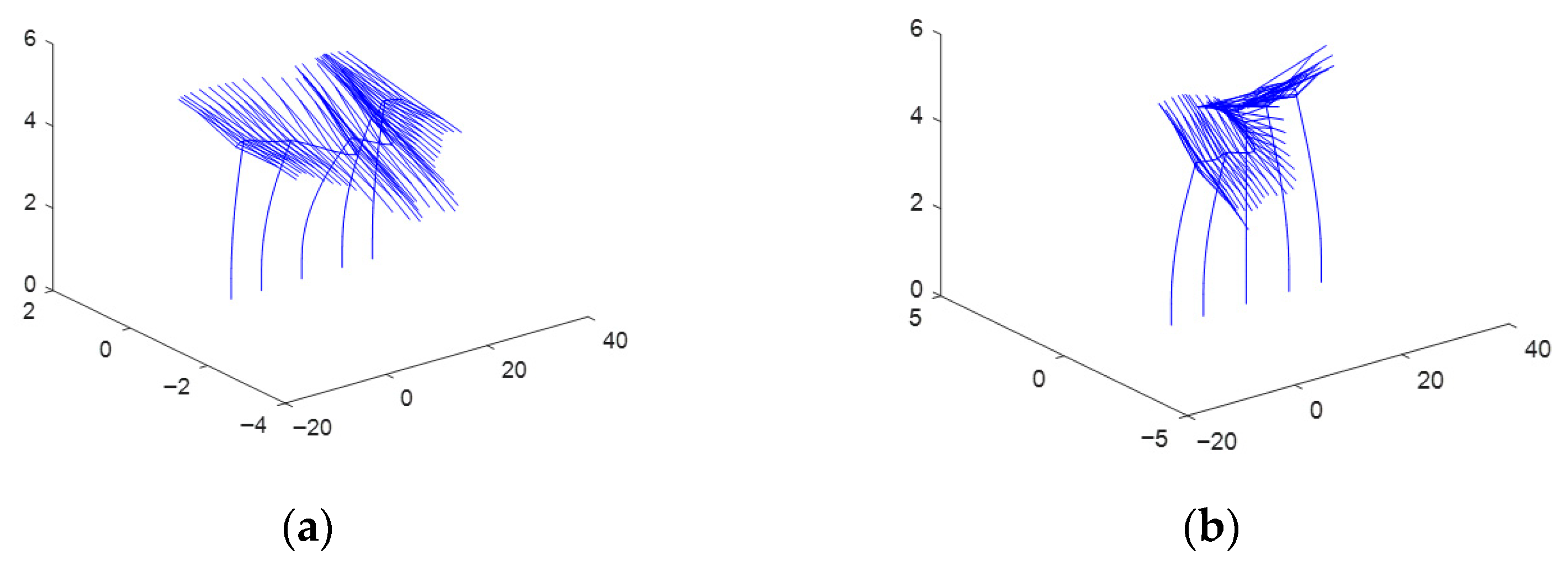
First, conduct a free-vibration analysis on the deterministic structure (i.e., take the design values for all parameters). The first five natural frequencies can be obtained as 0.304 Hz, 0.327 Hz, 0.348 Hz, 0.387 Hz, and 0.433 Hz respectively. The first five vibration modes are shown in Figure 11.

As can be seen from Figure 11, the first five vibration modes of the five-column HSSTB are mainly characterized by the lateral swing of the cantilever beam of the support column, with the maximum displacement concentrated at the free end. In each mode, the swing direction of each column is different, resulting in different bending forms of the main beam of the system. Specifically, in the first vibration mode, all five columns undergo lateral swinging, and the swing amplitude of the middle column is the largest. In the second vibration mode, the central column hardly shifts, and the two side columns swing around the central column. The third vibration mode is characterized by a small lateral shift of the second and fourth columns, while the side columns and the middle column swing in opposite directions. In the fourth vibration mode, the center column remains stationary, while the 1st, 4th, and 2nd, 5th columns swing in opposite directions respectively. The fifth vibration mode is that the side columns remain stationary, while the second, fourth columns and the center column swing in opposite directions respectively. In summary, the higher the mode, the more frequently the positive and negative lateral shifts at the top ends of each column will be switched. The first five modes are lateral bending modes of the frame. Modal mass participation results show negligible X/Z participation and a Y-direction (lateral) cumulative participation of 28.51% across modes 1–5 (Mode-wise: Y = 24.87%, 0.00%, 3.59%, 0.00%, 0.05%).

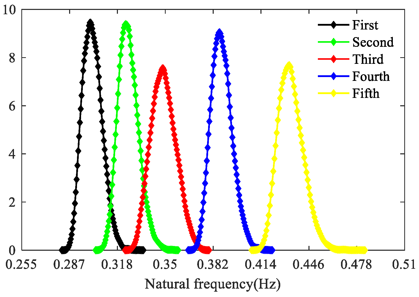
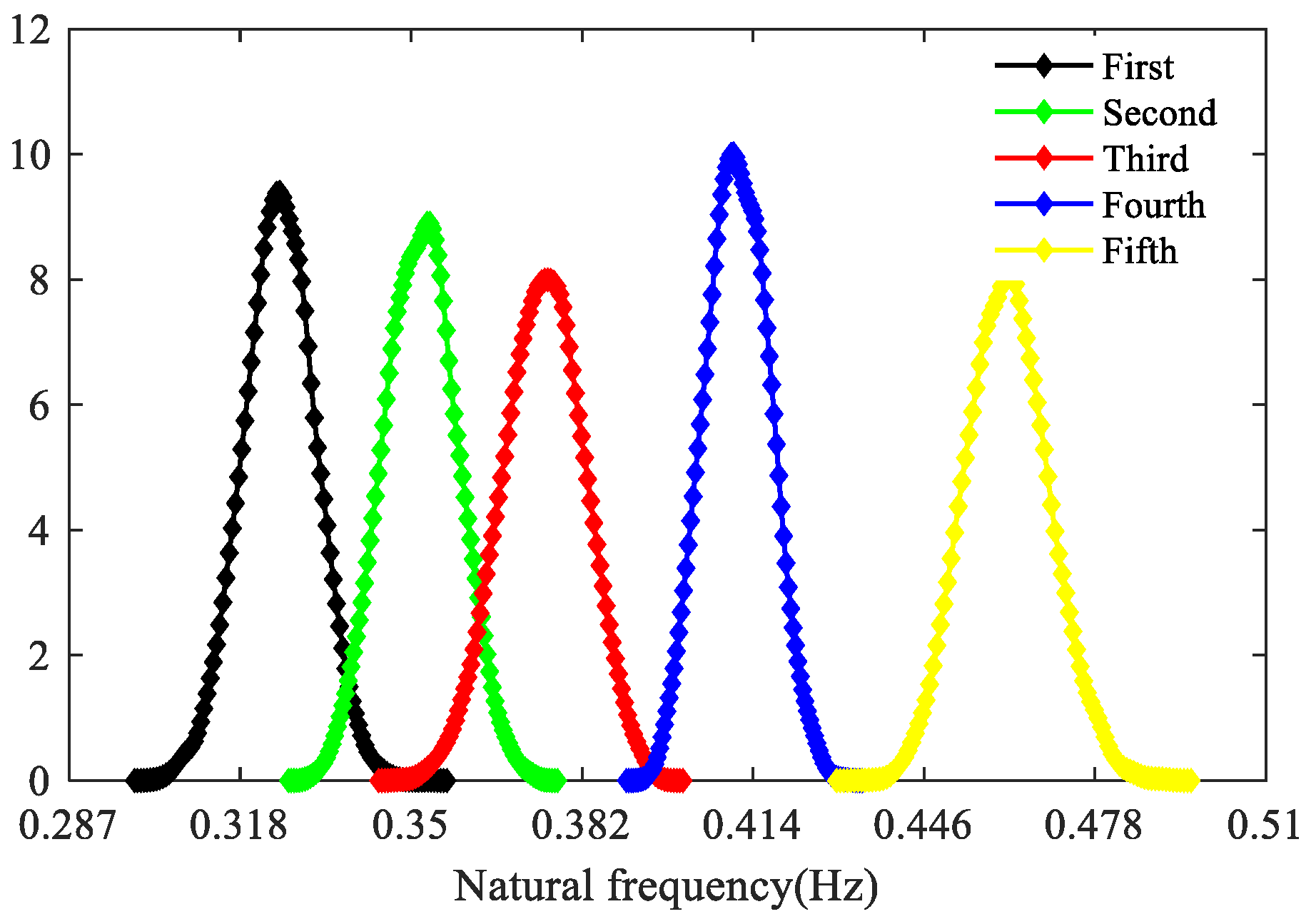
The probability densities of the first five natural frequencies are shown in Figure 12, with their mean values, variance, CoV and skewness showing in

Table 3. Statistical summary (mean, variance, CoV, skewness) of the first five natural frequencies of the unreinforced five-column HSSTB.

Mode	Mean	Variance	CoV	Skewness
1	0.3017	0.0016	0.0213	0.3657
2	0.3257	0.0012	0.0168	0.4391
3	0.3490	0.0020	0.0203	0.2063
4	0.3877	0.0013	0.0149	0.4057
5	0.4337	0.0015	0.0144	0.4722

. It can be seen that after considering the randomness of the parameters of the support column, the natural frequency of the structure will slightly decrease, that is, the flexibility of the structure will increase.

As can be seen from Figure 12, the probability densities of each natural frequency all show a unimodal distribution, and the samples at the right tail are more than those at the left tail, which is an asymmetric non-Gaussian distribution type. In addition, the CoV of the first five natural frequencies are 0.0213, 0.0168, 0.0203, 0.0149 and 0.0144 respectively, all of which are significantly less than the variability of the input random variables, indicating that the support system has certain inherent robustness.

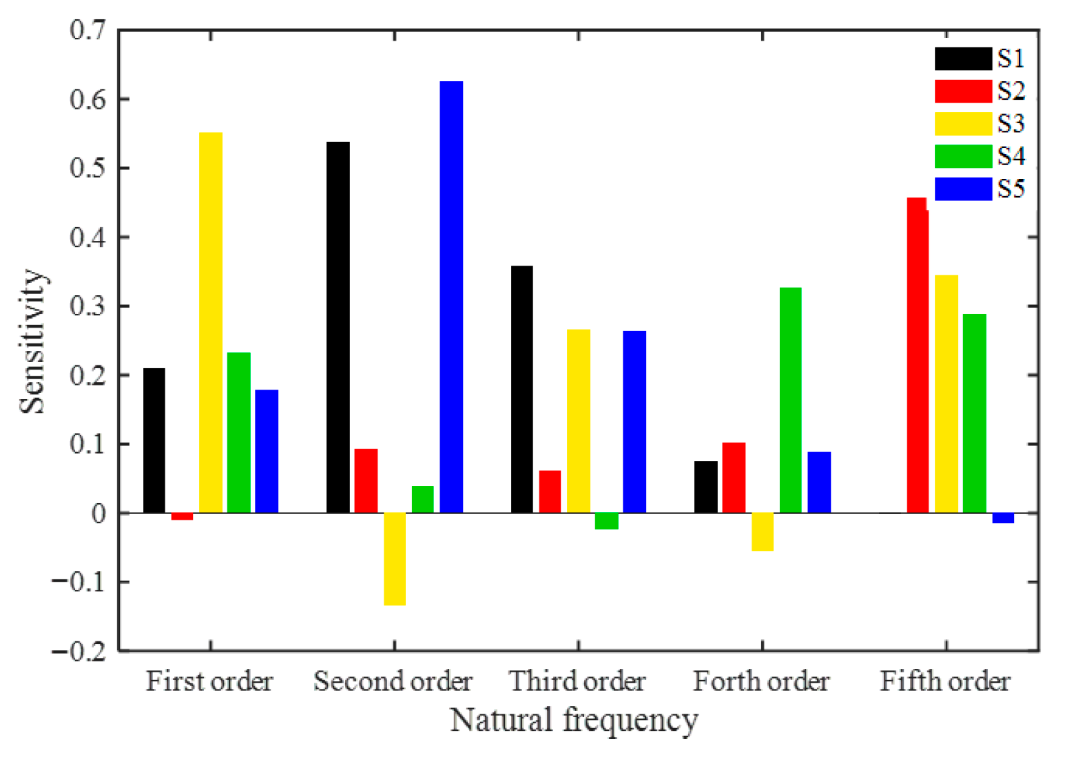
Figure 13 presents the global sensitivity analysis results of the first five natural frequency parameters. The global sensitivities of the five random variables are represented by S1–S5 respectively.

It can be seen that the 1st natural frequency is most sensitive to the randomness of the elastic modulus of the center column. The 2nd natural frequency is more sensitive to the elastic modulus of the two side columns. The sensitivity of the 3rd natural frequency to the elastic modulus of the first, third and fifth columns is relatively higher. The 4th natural frequency is mainly affected by the fourth pillar. The 5th natural frequency is more significantly affected by the three middle columns. In summary, the 1st, 4th and 5th natural frequencies of this support system are susceptible to the influence of the three middle columns, while the 2nd and 3rd natural frequencies are susceptible to the influence of the two side columns.

The observed Sobol’ rankings follow the modal strain-energy distribution. With the top beam rotationally restrained, the low-order response is governed by lateral (global-Y) bending. In Mode 1 (symmetric), the curvature envelope peaks near the central column(s); therefore, stiffness variability in the central column contributes the largest share to the frequency variance. In Modes 2–3 (anti-symmetric/mixed), larger curvature occurs toward the edge columns, which explains their higher indices in these modes. This central-vs-edge alternation is a direct consequence of the mode-shape phase relations and where bending energy is stored in each mode.

Table 4. First-order and total-effect Sobol’ indices for the first natural frequency of the unreinforced five-column HSSTB.

	ξ1	ξ2	ξ3	ξ4	ξ5
Si	0.210	0.012	0.552	0.231	0.179
STi	0.246	0.025	0.561	0.268	0.183

reports both the first-order and total-effect Sobol’ indices for the first natural frequency in the unreinforced five-column HSSTB. The results show that ξ₃ is the dominant contributor. Importantly, the differences between the first-order and total-effect Sobol’ indices are small across all variables (≈0.004–0.037), indicating weak higher-order interactions and an almost additive dependence of the frequency on the independent column-stiffness variables.

4.2.2. Global Sensitivity Analysis of Random Natural Vibration of the Five-Column HSSTB After Column Reinforcement

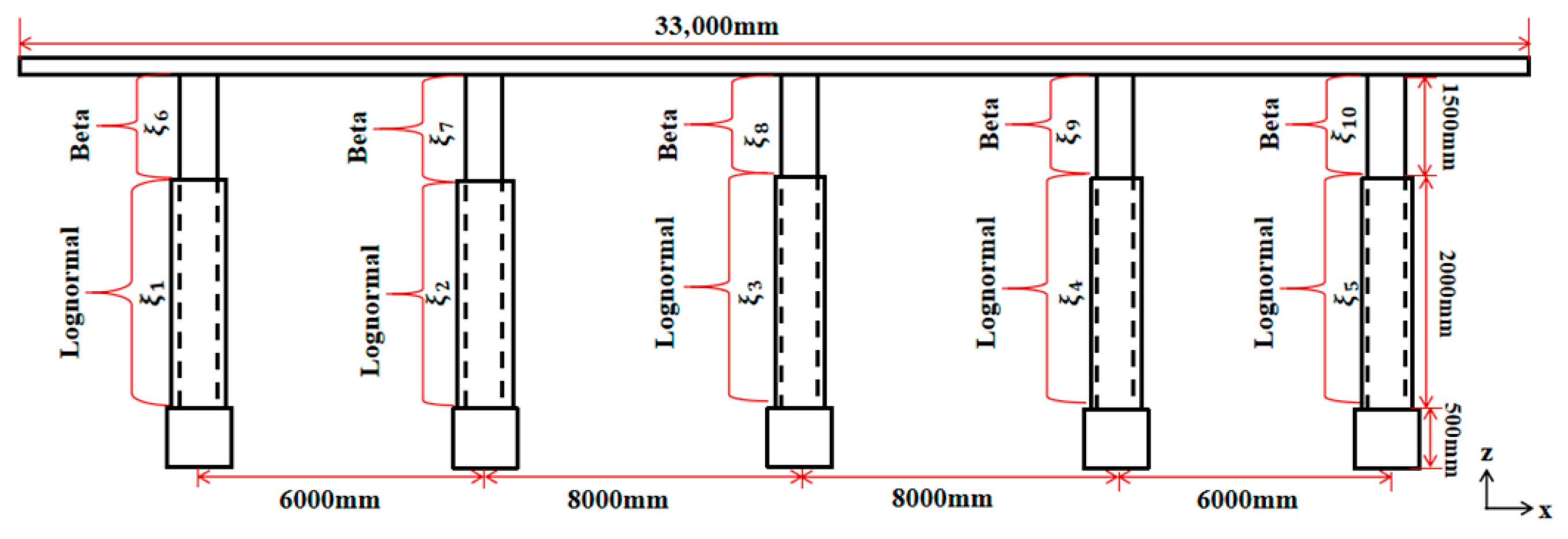
In order to enhance the stability of the solar support system and extend its service life, during the subsequent service of the five-column HSSTB, partial reinforcement treatment was carried out on the five columns, that is, a layer of channel steel was wrapped 2.5 m above the bottom of the column. The reinforcement was modeled by augmenting the original H-shaped steel column section with the cross-sectional properties of the channel steel. The channel steel was assumed to be perfectly bonded to the original column, simulating a full-strength connection as intended in the design. This was implemented in the FE model by modifying the sectional properties (area, moment of inertia) of the BEAM188 elements within the reinforced 2.5-m region at the column base. The reinforced support system is shown in Figure 14.

Suppose the elastic modulus of the reinforced parts of the five columns follows a log-normal distribution with a mean of 0 and a standard deviation of 0.1 after translation. The elastic modulus of the unreinforced part still follows a Beta distribution with a mean of 0 and a standard deviation of 0.1. The position distribution of the 10 random variables of the reinforced photovoltaic support system in the structure is shown in Figure 14.

Firstly, the first five natural frequencies of the structural parameters are calculated when taking the design values, which are 0.328 Hz, 0.354 Hz, 0.374 Hz, 0.410 Hz, and 0.460 Hz, respectively. The natural frequencies have slightly increased compared to those before reinforcement. Figure 15 presents the first five vibration modes of the photovoltaic support system after reinforcement when the parameters take the design values. Its vibration modes are basically the same as that of the vibration mode before reinforcement (see Figure 11). It can be seen from this that after simultaneously reinforcing the bottom of the five columns, the natural frequencies will increase, but it has little impact on the vibration modes.

The probability densities of the first five natural frequencies are shown in Figure 16, with their mean values being 0.3256 Hz, 0.3519 Hz, 0.3747 Hz, 0.4109 Hz, and 0.4611 Hz, respectively. The coefficients of variation are 0.0210, 0.0190, 0.0200, 0.0145, and 0.0169 respectively (as shown in

Table 5. Statistical summary (mean, variance, CoV, skewness) of the first five natural frequencies of the reinforced five-column HSSTB.

Mode	Mean	Variance	CoV	Skewness
1	0.3256	0.0018	0.0210	−0.0489
2	0.3519	0.0018	0.0190	0.0179
3	0.3747	0.0022	0.0200	−0.1103
4	0.4109	0.0014	0.0145	0.0514
5	0.4611	0.0024	0.0169	0.1411

), all of which are less than the variability in the input parameters.

Figure 17 presents the global sensitivity analysis results of the parameters of the first five natural frequencies after enhancement. The sensitivities of the 10 random variables are represented as S1–S10.

As can be seen from Figure 17, the first natural frequency is most sensitive to the randomness of the elastic modulus of the central column reinforcement part. The second natural frequency is more sensitive to the elastic modulus of the reinforced parts of the two side columns. The sensitivity of the third and fourth natural frequencies to the parameters is close, and both are relatively more sensitive to the elastic modulus of the reinforced parts of the first, second, and fifth columns. The fifth natural frequency is more significantly affected by the elastic modulus of the reinforced parts of the three middle columns. In summary, the natural frequency of the reinforced photovoltaic support is mainly affected by the elastic modulus of the reinforced part, while the influence of the elastic modulus of the upper unreinforced part is very small. This is because the reinforced part will directly affect the natural vibration characteristics of the structure.

Jacketing the lower 2.5 m of each column increases base stiffness, reduces base-region compliance, and redistributes the modal curvature along the members. Consequently, the mean natural frequencies increase and the Sobol shares re-allocate: the previously dominant column’s contribution may decrease as its variability is less effective in altering the global stiffness, while other columns’ contributions may increase or the ranking may partially shift, depending on how the strengthened base relocates the curvature envelopes for each mode. This mechanism is consistent with the Y-direction modal mass participation and with the experimental validation, confirming that lateral-bending control remains the governing feature under the restrained-beam configuration.

Compared with the five-column HSSTB before enhancement, the influencing factors of the first, second, and fifth frequencies of the structure are basically the same, while the sensitivity of the third and fourth natural frequencies to the parameters is different. The dynamic stability of the HSSTB under wind load is often affected by the higher vibration modes. Therefore, after reinforcement, special attention should be paid to the sensitivity changes in the higher vibration modes. This is extremely crucial for the stability analysis of the HSSTB structures under wind loads.

5. Conclusions

This paper takes an HSSTB in Gansu Province, China, as an example. Considering the randomness of the elastic modulus of the steel column, the Kriging method is used to study the free-vibration characteristics of the five-column HSSTB and analyze the global sensitivity of parameters. The following conclusions can be drawn:

For the five-column HSSTB examined here, the low-order free-vibration behavior is governed by lateral bending under the top-beam rotationally restrained condition. In the unreinforced configuration, Sobol indices indicate that the central column is the dominant contributor to the first natural frequency (Mode 1), whereas the edge columns contribute more to Modes 2–3; Modes 4–5 show mixed influence among the middle columns. After jacketing the lower 2.5 m of each column, the mean natural frequencies increase by 6–8% (Modes 1–5), and the reinforced segments become the primary stiffness drivers, while the qualitative ranking of “central vs. edge” influence remains largely consistent for Modes 1, 2, and 5. These findings support the following practical recommendations: prioritize reinforcement and monitoring of the central column for Mode 1 control; include edge columns when targeting Modes 2–3; and, when retrofitting, stiffen the lower 2–3 m of the columns to achieve meaningful gains in the fundamental frequency. For condition assessment, periodic ambient-vibration measurements at column-top locations are efficient for tracking lateral bending modes and detecting stiffness changes.

It is important to note that this study assumed a fixed base condition for the concrete foundations. In reality, soil–structure interactions can influence the dynamic characteristics of the system. The incorporation of foundation flexibility using, for example, spring elements based on site-specific geotechnical data represents an important direction for future research to further refine the model’s accuracy. In future work, we will extend the framework to (i) model the elastic modulus as a spatial random field with identifiable correlation lengths and (ii) incorporate uncertainties in cross-sectional dimensions, pile–soil interaction (SSI), and damping. These additions will provide a more comprehensive quantification of variability and its impact on modal properties.

References

1. Zhu, H.; Wang, Y.; Wu, J.; Zhang, X. A regional distributed photovoltaic power generation forecasting method based on grid division and TCN-Bilstm. Renew. Energy 2026, 256, 123935. [Google Scholar] [CrossRef]
2. Hou, Z.; Zhang, Y.; Cheng, X.; Ye, X. Photovoltaic Power Forecasting Based on Variational Mode Decomposition and Long Short-Term Memory Neural Network. Energies 2025, 18, 3572. [Google Scholar] [CrossRef]
3. Jia, M.; Hu, W.; Zhang, X.; Dai, X.; Lei, Z.; Zhou, H. A multi-source data-driven approach for online photovoltaic power prediction. Electr. Power Syst. Res. 2025, 248, 111913. [Google Scholar] [CrossRef]
4. Wu, S.; Wu, H.; Lou, Y. Analysis of the response of wind-induced vibrations on flexible photovoltaic mounts. J. Phys. Conf. Ser. 2024, 2865, 012057. [Google Scholar] [CrossRef]
5. Gong, B.; Li, Z.; Wang, Z.; Wang, Y. Wind-induced dynamic response of Heliostat. Renew. Energy 2012, 38, 206–213. [Google Scholar] [CrossRef]
6. Ferroudji, F.; Khelifi, C.; Outtas, T. Structural dynamics analysis of three-dimensional bi-axial sun-tracking system structure determined by numerical modal analysis. J. Sol. Energy Eng. 2018, 140, 031004. [Google Scholar] [CrossRef]
7. Ji, B.; Xing, P.; Xu, F.; Xiong, Q.; Qiu, P.; Liu, Q.; Tan, D. Transient Evaluation of Wind-Induced Vibration Response of Heliostat Under Downburst. Energy Technol. 2023, 11, 2300156. [Google Scholar] [CrossRef]
8. Davenport, A.G. Gust Loading Factors. J. Struct. Div. 1967, 93, 11–34. [Google Scholar] [CrossRef]
9. Liu, J.; Li, S.; Luo, J.; Chen, Z. Experimental study on critical wind velocity of a 33-meter-span flexible photovoltaic support structure and its mitigation. J. Wind. Eng. Ind. Aerodyn. 2023, 236, 105355. [Google Scholar] [CrossRef]
10. Chen, F.; Zhu, Y.; Wang, W.; Shu, Z.; Li, Y. A Review on Aerodynamic Characteristics and Wind-Induced Response of Flexible Support Photovoltaic System. Atmosphere 2023, 14, 731. [Google Scholar] [CrossRef]
11. Hamdaoui, M.; Daya, E.M. Global sensitivity analysis of damped sandwich plates using sparse polynomial chaos expansions. Mech. Adv. Mater. Struct. 2025, 32, 2807–2821. [Google Scholar] [CrossRef]
12. Du, S.; Ellingwood, R.; Cox, V. Solution methods and initialization techniques in SFE analysis of structural stability. Probabilistic Eng. Mech. 2005, 20, 179–187. [Google Scholar] [CrossRef]
13. Ghienne, M.; Nennig, B. Beyond the limitations of perturbation methods for real random eigenvalue problems using Exceptional Points and analytic continuation. J. Sound Vib. 2020, 480, 115398. [Google Scholar] [CrossRef]
14. Kamiński, M.; Świta, P. Generalized stochastic finite element method in elastic stability problems. Comput. Struct. 2011, 89, 1241–1252. [Google Scholar] [CrossRef]
15. Lamouri, H.; Mkhalet, E.; Lamdouar, N. Reliability polynomial chaos metamodel for the dynamic behaviour of reinforced concrete bridges. Adv. Bridge Eng. 2024, 5, 27. [Google Scholar] [CrossRef]
16. Zhang, H.; Huang, B.; Liu, Y.; Xiang, X.; Wu, Z. A new stochastic residual error based homotopy approach for stability analysis of structures with large fluctuation of random parameters. Int. J. Numer. Methods Eng. 2023, 124, 183–216. [Google Scholar] [CrossRef]
17. Zhang, H.; Xiang, X.; Huang, B.; Wu, Z.; Chen, H. Static homotopy response analysis of structure with random variables of arbitrary distributions by minimizing stochastic residual error. Comput. Struct. 2023, 288, 107153. [Google Scholar] [CrossRef]
18. Zhang, H.; Liu, Y.; Huang, B.; Wu, X.; Wu, Z.; Michael, H. Dynamic characteristics of vertically irregular structures with random fields of different probability distributions based on stochastic homotopy method. Mech. Syst. Signal Process. 2024, 220, 111638. [Google Scholar] [CrossRef]
19. Chiron, M.; Morio, J.; Dubreuil, S. Local Sensitivity of Failure Probability through Polynomial Regression and Importance Sampling. Mathematics 2023, 11, 4357. [Google Scholar] [CrossRef]
20. Wang, Q.; Wu, D.; Tin-Loi, F.; Gao, W. Machine learning aided stochastic structural free vibration analysis for functionally graded bar-type structures. Thin-Walled Struct. 2019, 144, 106315. [Google Scholar] [CrossRef]
21. Laudani, R.; Falsone, G. Closed-form expressions for eigenvalue and eigenvectors of stochastic symmetric matrices using the probability transformation method. Probabilistic Eng. Mech. 2024, 78, 103706. [Google Scholar] [CrossRef]
22. Zheng, Z.; Beer, M.; Nackenhorst, U. Efficient stochastic modal decomposition methods to solve stochastic structural static and dynamic problems. Int. J. Numer. Methods Eng. 2024, 125, 7469. [Google Scholar] [CrossRef]
23. Taliadouros, L.; Mavromatis, I.; Kougioumtzoglou, I. Eigenvalue analysis of stochastic structural systems: A quantum computing approach. Probabilistic Eng. Mech. 2025, 81, 103814. [Google Scholar] [CrossRef]
24. Wang, L.; Li, G.; Lu, Z.; Feng, K. Local sensitivity analysis of failure possibility and its universal solution by fuzzy simulation. Struct. Multidiscip. Optim. 2021, 64, 1–20. [Google Scholar] [CrossRef]
25. Sudret, B.; Mai, C. Computing derivative-based global sensitivity measures using polynomial chaos expansions. Reliab. Eng. Syst. Saf. 2015, 134, 241–250. [Google Scholar] [CrossRef]
26. Sobol, I.M. Sensitivity analysis for nonlinear mathematical models. Appl. Math. Model. 1990, 2, 112–118. [Google Scholar]
27. Liu, F.; Wei, P.; Tang, C.; Wang, P.; Yue, Z. Global sensitivity analysis for multivariate outputs based on multiple response Gaussian process model. Reliab. Eng. Syst. Saf. 2019, 189, 287–298. [Google Scholar] [CrossRef]
28. Novak, L. On distribution-based global sensitivity analysis by polynomial chaos expansion. Comput. Struct. 2022, 267, 106808. [Google Scholar] [CrossRef]
29. Chen, J.; Wan, Z.; Beer, M. A global sensitivity index based on Frechet derivative and its efficient numerical analysis. Probabilistic Eng. Mech. 2020, 62, 103096. [Google Scholar] [CrossRef]
30. Wan, Z. Global sensitivity evolution equation of the Frechet-derivative-based global sensitivity analysis. Struct. Saf. 2024, 106, 102413. [Google Scholar] [CrossRef]
31. Wang, B.; Luo, L.; Nie, X.; Duan, S.; Likai, W. Post-buckling Reliability and Sensitivity Analysis of Composite Stiffened Plates Based on Adaptive Kriging Method. Acta Mech. Solida Sin. 2023, 36, 340–348. [Google Scholar] [CrossRef]
32. Mohammad, F.; Ammar, A.; Mu’ath, I. Sensitivity and reliability assessment of buckling restrained braces using machine learning assisted-simulation. J. Constr. Steel Res. 2023, 211, 108187. [Google Scholar] [CrossRef]
33. Leblouba, M.; Barakat, S.; Al-Saadon, Z. Shear behavior of corrugated web panels and sensitivity analysis. J. Constr. Steel Res. 2018, 151, 94–107. [Google Scholar] [CrossRef]
Figure 1. Horizontal single-axis solar tracking bracket (HSSTB) at a photovoltaic site in Gansu Province, China.
Processes 13 03489 g001
Figure 2. Five-column HSSTB: (a) finite-element model of the five-column HSSTB; (b) on-site five-column HSSTB structure at the project site.
Processes 13 03489 g002
Figure 3. (a) Front elevation view of the five-column HSSTB. (b) Side elevation view of the five-column HSSTB. (c) Cross-section of the concrete base. (d) Cross-section of the main beam. (e) Cross-section of the support column. (f) Cross-section of the diagonal brace. (g) Cross-section of the roof purlin.
Processes 13 03489 g003
Figure 4. On-site ambient vibration test of the reinforced five-column HSSTB.
Processes 13 03489 g004
Figure 5. Geometric dimensions for the single reinforced photovoltaic steel column case: (a) side elevation of the column; (b) cross-sectional geometry of the upper I-section; (c) cross-sectional geometry of the lower reinforced section.
Processes 13 03489 g005
Figure 6. Sobol indices for the first three natural frequencies of the single-column photovoltaic steel column under the small-variability case (CoV = 0.10): (ac) Mode 1; (df) Mode 2; (gi) Mode 3. Indices are obtained from the Kriging surrogate with increasing training sample sizes.
Processes 13 03489 g006
Figure 7. Sobol indices for the first three natural frequencies of the single-column photovoltaic steel column under the moderate-variability case (CoV = 0.25): (ac) Mode 1; (df) Mode 2; (gi) Mode 3. Indices are obtained from the Kriging surrogate with increasing training sample sizes.
Processes 13 03489 g007aProcesses 13 03489 g007b
Figure 8. Sobol indices of the first three natural frequencies under small variation: (a) first natural frequency; (b) second natural frequency; (c) third natural frequency.
Processes 13 03489 g008
Figure 9. Sobol indices of the first three natural frequencies under moderate variation: (a) first natural frequency; (b) second natural frequency; (c) third natural frequency.
Processes 13 03489 g009
Figure 10. Kriging validation for the first natural frequency of the unreinforced five-column HSSTB: parity plot of Kriging-predicted vs. true frequencies (Hz).
Processes 13 03489 g010
Figure 11. First five free-vibration mode shapes of the five-column HSSTB in the unreinforced deterministic configuration: (a) Mode 1; (b) Mode 2; (c) Mode 3; (d) Mode 4; (e) Mode 5.
Processes 13 03489 g011
Figure 12. Probability density functions of the first five natural frequencies for the unreinforced five-column HSSTB.
Processes 13 03489 g012
Figure 13. Sobol’ indices for the first five natural frequencies of the unreinforced five-column HSSTB.
Processes 13 03489 g013
Figure 14. Cross-section view of the enhanced five-column HSSTB.
Processes 13 03489 g014
Figure 15. The first five vibration modes of the five-column HSSTB with deterministic parameters after reinforcement.
Processes 13 03489 g015aProcesses 13 03489 g015b
Figure 16. Probability density distributions of the first five natural frequencies.
Processes 13 03489 g016
Figure 17. Sobol indices of the first five natural frequencies.
Processes 13 03489 g017