Abstract
This article demonstrates how the non-intrusive techniques PLIF (Planar Laser-Induced Fluorescence) and PIV (Particle Image Velocimetry) are used to study fluid flow and mixing in a water model of a continuous casting tundish. These techniques validate CFD models by providing hydrodynamic data and by testing the models’ ability to predict mixing through simulated concentration field evolution under defined process conditions. Using PIV and PLIF yields more accurate information on turbulent mixing and impurity transport than traditional methods. Access to flow and concentration field evolution enables more precise mathematical model refinement and clarifies the impact of tundish design or operational changes on hydrodynamics and mixing. Relative errors in chemical evolution are approximately 20%, whereas velocity errors vary depending on the measurement plane, being lower for longitudinal planes and higher for transversal planes. This suggests that the turbulence model does not fully capture all low- and high-velocity zones. This approach supports reliable flow and mixing predictions in metallurgy and related fields.
1. Introduction
The continuous steel casting tundish is a metallurgical reactor that has played a central role in advancing high-quality steel production. Despite the abundance of research, a key issue is understanding how physical and numerical modeling have driven innovations in tundish performance. Researchers have focused on flow control and mixing, especially through the evaluation of flow-modifying devices with both mathematical and experimental approaches. The extensive study of Residence Time Distribution (RTD) curves and F curves has been crucial to optimizing chemical and thermal mixing in these reactors.
Three major literature reviews by Guthrie and Mazumdar, covering 185 articles, trace how advances in physical and mathematical modeling have informed tundish operations from 1970s to 2019 [1,2,3]. By categorizing research into physical, mathematical, and combined modeling, these reviews establish how systematic modeling analysis has been foundational to driving technical improvements in tundish processes.
Reliable experimental data on flow and mixing for the tundish’s specific design and conditions is key to adjusting and improving CFD models. That is why using LDA (Laser Doppler Anemometry) or PIV (Particle Image Velocimetry) to measure flow, along with standard ways to obtain RTD curves, has been essential for refining CFD modeling in tundishes.
Due to the importance of using physical and numerical modeling to improve tundish performance, interest in developing new improvement proposals using these tools has continued, as revealed by recent publications regarding changes in tundish design and operating conditions. Rajasekar and Kumar [4] studied three arrangements by adding flow modifiers to improve a 40-ton slab caster tundish. This tundish consisted of a pouring box, a weir, and a dam. Using physical and numerical modeling, all configurations improved performance compared to the base case. In a related study, Yue et al. [5] used physical modeling and the internal RTD method to evaluate fluid mixing in a multi-flow continuous casting tundish. Their analysis showed that adding a dam to the tundish’s impact zone decreased the dead zone volume fraction. Similarly, Constantino et al. [6] used physical modeling to determine the residence time distribution, minimum and maximum concentrations, and active and dead volume fractions in a 5-strand asymmetric tundish equipped with turbulence inhibitors and argon curtains.
Maurya et al. [7] studied how different ladle shroud designs affect the flow in the steelmaking tundish and the size of the open eye using experiments and computer models. They found that the ladle shroud design can greatly improve tundish flow.
Complementing these efforts to modify tundish performance, Zhang et al. [8] propose installing a turbulent swirling flow generator (SFG) around the inlet of the submerged inlet nozzle by injecting air bubbles into the turbulent flow field to remove inclusions. Their computational fluid dynamics (CFD) simulation results show that the application of SFG could dramatically improve the efficiency of inclusion removal.
Building on previous research, Sheng [9] developed a conjugate heat transfer CFD model to analyze fluid flow and temperature distributions in molten steel within a single-strand tundish. Specifically, the study focused on heat transfer through linings and tundish covering flux (TCF). The results indicate that reducing the insulation layer’s thermal conductivity and increasing the TCF layer’s thickness effectively minimize heat loss compared to an uncovered tundish.
These advances converge in efforts such as those of Demeter et al. [10], who presented a detailed numerical analysis to design an optimally shaped impact pad into a tundish. They assess the effectiveness of each proposed design through a tracer-based visualization of flow behavior and the evaluation of RTD curves. A real plant trial test verified the results of the simulations. Results show that using a specific impact pad can significantly enhance the flow characteristics of liquid steel during the continuous casting process.
In addition to advances in tundish design, researchers have shown special interest in improving characterization techniques used in physical modeling. These advances aim to generate reference information to validate CFD numerical models.
Dinda et al. [11] used experiments to study how tracer concentration affects RTD results. They found that the tracer concentration has a big effect on the measured dead zone in the RTD analysis. They found that the root cause of wrong RTD results is the flow in the tundish, which changes with density differences caused by the tracer.
Geng et al. [12] use physical modeling to study the volume effect of saturated KCl solution and KCl solution–ethanol mixed improved tracer in a bare single-strand tundish. They found that, unlike the behavior of saturated KCl, the volume effect of specific improved tracers on the flow field in the tundish can be relatively weak and neglected, thus minimizing experimental errors and accurately representing the flow characteristics within the tundish.
In seeking reliable alternatives for characterizing flow, Li et al. [13] propose a methodology for characterizing tundish flow fields by integrating ink diffusion experiments with digital image processing techniques. Comparative validation against PIV measurements demonstrated good agreement between the two methods, with a minimum relative error of 9% between the velocities obtained from this approach and those measured by PIV.
Novel experimental techniques like PLIF (Planar Laser-Induced Fluorescence) and PIV (Particle Image Velocimetry) can measure chemical and thermal mixing as well as fluid flow. Specifically, chemical PLIF provides detailed data on the evolution of solute mass transfer mechanisms in the system, which, in turn, enables a thorough, quantitative study of the turbulent diffusion and convection mechanisms controlling mixing kinetics. Furthermore, this information is valuable for both validating numerical CFD models from a hydrodynamic perspective and testing their ability to predict mixing by simulating the evolution of concentration fields under specific process conditions.
Combining PIV and PLIF may provide more in-depth and detailed research into how tundish design and operating condition changes affect hydrodynamics and mixing behavior. This, in turn, helps propose improved designs and operating conditions for industrial tundishes. Despite these advantages, only four studies have examined chemical PLIF in physical tundish modeling due to technical difficulties in implementation.
Few published works exist on using chemical PLIF to model tundishes. This scarcity suggests it is a promising research area for studying mixing kinetics. Thus, this work seeks to help fill the gap that has, until now, prevented the generation of reliable experimental data on how solute fields evolve in physical tundish models.
Koitzsch et al. [14] used a physical model of a single-thread tundish without flow modifiers. They applied PIV/PLIF techniques to characterize the flow structure and measure the evolution of concentration fields in two longitudinal planes and one transverse plane within the model. They also obtained the RTD curve using the concentrations detected by the PLIF just above the tundish outlet. They compared it with the RTD curve obtained using the conventional tracer injection technique and with that generated by a CFD model to validate it.
Braun and Pfeifer [15] employed PIV/PLIF methods to investigate the impact of interrupting the flow at one of the outlets of a two-thread tundish physical model on the system’s flow structure and mixing process. They obtained the evolution of the flow structure and concentration fields in half of the longitudinal symmetry plane of the model. They found that interrupting the casting process in one of the molds changes the flow structure’s characteristics and affects the fluid’s mixing process inside the tundish.
Cwudzinski et al. [16] studied how changing the location and number of alloying addition points affects chemical homogenization in a tundish. They used a physical model of a tundish and four different tracer addition modes. They used the conventional pulse method to determine the mixing time for each addition mode. In the regions close to the tracer addition point, they determined the flow structure and mixing kinetics using PIV/PLIF techniques. They found that mixing times depend on the addition mode and that the observed changes in mixing times can be attributed to changes in flow structure and mixing kinetics near the addition points.
Due to technical problems with PLIF implementation and calibration in tundishes, Koitzsch et al. [14] and Braun & Pfeifer [15] used a system saturated with solute and injected solvent (water) to study how the solute dissolved over time. Similarly, because of these challenges, Cwudzinski et al. [16] only characterized the immediate area around tracer addition points using PIV/PLIF.
In our previous work [17], we adapted a PLIF calibration procedure, originally developed for gas-stirred ladles, to measure instantaneous concentration fields in a tundish. This solved PLIF technique issues that had hindered implementation, such as nonuniform illumination and shadows created by acrylic wall imperfections. This work uses that methodology [17] to implement PIV/PLIF in a tundish physical model. The evolution of flow and concentration fields in a transverse plane serves to adjust a CFD model intended to simulate the system.
Accordingly, this work extensively validated a mathematical model through PIV and PLIF measurements. The model predicts fluid flow, convection, and turbulent dispersion of chemical species in a water physical model of a two-strand tundish. The results indicate that PLIF, in conjunction with PIV, helped verify and fine-tune a mathematical model. Therefore, the work suggests a robust route for future investigations in combined physical and mathematical studies to understand the physics governing complex processes, such as chemical mixing in a tundish.
2. Materials and Methods
2.1. Mathematical Modeling
In this work, non-intrusive experimental techniques were employed to measure the flow field (PIV) and mixing (PLIF) within a physical model of a two-strand tundish constructed without flow modifiers. The physical model simulated was constructed with a scale factor of 1:3, referring to a 16-ton industrial prototype. The dimensions of the physical model are detailed in [17] and in the next section. A three-dimensional mathematical model was developed to calculate and compare the fluid flow and mixing inside the tundish physical model. The use of experimental optical techniques will help validate the mathematical model by comparing the results of the physical and mathematical models side by side.
The model uses mass and momentum conservation, the realizable k-ε turbulence model, and species transport equations. The main assumptions are: (i) fluid flow is steady-state; tracer mixing is solved in transient-state after fluid flow calculation, (ii) two symmetry planes are used, so only one-quarter of the tundish is modeled, (iii) the free surface remains flat and fixed, (iv) water and its rhodamine solution are incompressible, Newtonian fluids, (v) rhodamine dissolves in water without altering its properties and does not chemically react, (vi) temperature variations and their fluid property effects are neglected, (vii) walls have no-slip condition, connecting turbulent core with laminar walls via standard wall functions, and (viii) turbulence is modeled by the realizable k-ε turbulence model. There are better options to simulate turbulence, like the LES (Large Eddy Simulation) which allows for the presence of small- and medium-sized transient flow structures, called Eddies, which improve the accuracy of the flow field calculations due to the direct turbulence simulation. However, for the LES model to work properly, a very fine grid is needed. In recent works, the LES model has been successfully used in small sections of the tundish, such as the submerged entry nozzle, with meshes of 10 million elements [18]. In this work, a simulation of the whole tundish is resolved, so it is not feasible to use LES with our current computational resources. Considering this, we decided to use a Reynolds-averaged Navier–Stokes (RANS)-based turbulence model, specifically the realizable k-ε that has been previously reported to accurately simulate the fluid flow of tundishes in the literature [9,19].
- (a)
- Mass conservation equation:where is the mean velocity vector.
- (b)
- Momentum conservation equation:where ρ is the density, is the static pressure, is the stress tensor, and are the gravitational body force. The stress tensor is given by:where is the molecular viscosity and the transpose of the velocity vector.
- (c)
- Realizable - model equation:
After systematic validation trials, in which we tested all available turbulence models in the CFD software ANSYS Fluent™ 2023 R2 (Southpointe 2600 Ansys Drive Canonsburg, PA 15317, USA), the best model that matched the experimental results was the realizable k-ε turbulence model, which is the selection for this work.
where and are the turbulent kinetic energy and its dissipation rate, is the turbulent viscosity, the generation of turbulence kinetic energy due to the mean velocity gradients, and are turbulent Prandtl numbers for and , respectively, with values of 1 and 1.2, and is a constant with a value of 1.9. is calculated according to Equation (6).
And
where
- (d)
- Species transport equation:where is the velocity of the transported species, local mass fraction of each species, is the diffusion flux of species , while is calculated as follows:where is the mass diffusion coefficient for species in the mixture, and is the turbulent Schmidt number calculated as:
The boundary conditions include non-slip conditions at the bottom and lateral walls of the tundish and at the lateral wall of the shroud. Standard wall functions have been used to connect the turbulent core of the fluid with the laminar flow near the walls. A constant mass flow was used at the inlet, and an outflow boundary condition was applied at the outlet. The free surface was treated as a plane of symmetry. For the unsteady study of the injection of rhodamine as a tracer, a spherical region of 3 mL volume was patched close to the inlet to simulate the injection of rhodamine. At the same time, the rest of the boundaries, except the outlet, have zero flux of rhodamine because the rhodamine is free to leave the tundish at the outlet. The species transport equation’s initial condition assumes zero concentration of rhodamine in the entire system. Table 1 provides a more detailed description of the boundary conditions, while Figure 1a offers a schematic representation of the tundish, highlighting the boundaries.

Table 1.
Boundary conditions of the computational domain.
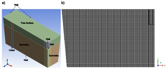
Figure 1.
(a) Boundary conditions of the computational domain, (b) Domain mesh on the symmetry plane xy.
The model was solved using ANSYS Fluent™ 2023 R2. A mesh with approximately 986,000 elements, featuring average orthogonal quality and aspect ratios of 0.98 and 1.12, respectively, was constructed as shown in Figure 1b, resulting from a grid sensitivity study. The study utilized 5 grids, as listed in Table 2, where the number of elements, quality features (including orthogonal quality and aspect ratio), and calculation time are presented. As shown in Figure 2, a comparison of the fluid velocity profiles obtained from all grids along a horizontal line from the center of the water inlet (0.0 m symmetry plane) to the lateral wall (0.5 m) at 0.10 m height of the tundish was performed, showing that a grid with 880,000 elements warrants that the velocity does not depend on the grid, but the 986,000-elements grid was selected because it must have better accuracy, and under the conditions we ran for the simulations, the time taken to reach convergence was the same as the previous mesh (880,000). The calculations were performed in a CPU (Dell precision T5600, Dell Way 1 Round Rock, TX 78682, USA.) with an Intel® Xeon® Silver 20-core at 2.40 Ghz processor, with 16 GB of RAM. The governing equations were solved using the SIMPLE algorithm for the coupling of the velocity and pressure fields. All simulations used a time step of 0.1 s, spatial discretization for pressure was PRESTO, for momentum equations was second-order upwind, and for turbulent kinetic energy and its dissipation rate was first-order upwind. The calculation time for solving the fluid flow in steady state was 15 min, and for solving the species transfer in transient-state was 3 h, which was sufficient to simulate 150 s of the tracer mixing. In both calculations, the convergence criteria were set as 10−3 for every governing equation residual.
Table 2.
Grid sensitivity study.
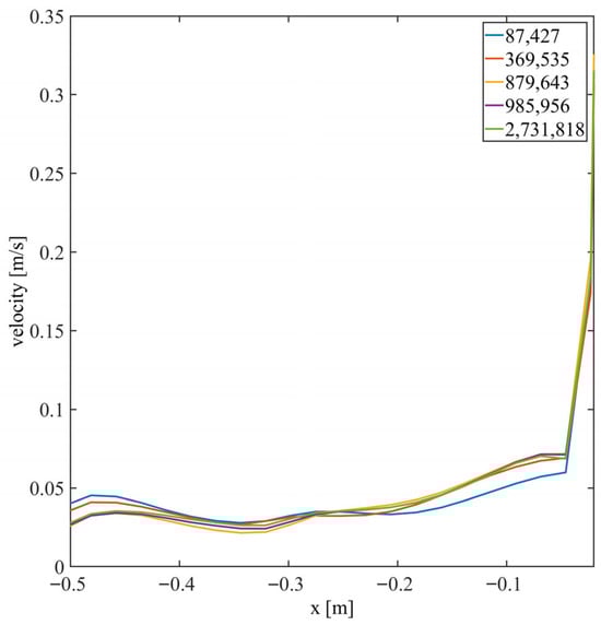
Figure 2.
Grid sensitivity study. Velocity profile of the fluid along a horizontal line from the center of the water inlet (0.0 m) to the lateral wall (0.5 m) at a height of 0.10 m for all the different grids.
2.2. Physical Modeling
An acrylic water physical model was designed to satisfy the relevant similarity criteria of a two-strand industrial prototype of 16-ton capacity [17]. Similarity criteria involved the geometric similarity by a scale factor of 1/3, kinematic similarity (similar velocities with similar forces) and dynamic similarity, ensuring the dimensionless group of forces driving the fluid are properly scaled (in this case the Froude number was equalized between the model and the industrial prototype), so the physical model reliably represents the behavior of the real system in terms of fluid dynamics. Flow modifiers were not employed to implement the PIV/PLIF in the simplest possible tundish system, and the focus was on the PLIF–PIV tools to fine-tune the model. Dimensions of the model are as follows: tundish length () 1.05 , tundish width () 0.26 , filling level for steady-state casting (H) 0.27 m, volume of tundish at filling () 0.084 , distance shroud-bottom () 0.20 m, and diameter of shroud () 0.023 . Distilled water at room temperature is used to simulate molten low-carbon steel at 1600 °C, taking advantage of the fact that both fluids possess almost identical kinematic viscosities, helping to meet the kinematic similarity (, ). The dynamic similarity is achieved by equating the Froude number in the prototype and the physical model to a value of 0.7394, as calculated by Equation (21).
where is the steel velocity at the shroud, is gravity constant and is the steady-state level of steel in the tundish.
The model operates continuously with two strands. The ladle shroud is in the center of the tundish at an equal distance from each outlet, and the water flow rate is 30 LPM (liters per minute) with a velocity of 1.2034 m/s to keep the water level steady at 0.27 m. Figure 3 presents a schematic of the model, showing top, lateral, and frontal views. Table 3 provides a more precise description of the measurement planes’ locations.
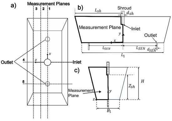
Figure 3.
Physical Model Tundish. (a) Top view, (b) Front view, (c) Lateral view.
Table 3.
Locations of measurements planes.
The particle image velocity (PIV) technique was used to measure the fluid dynamics in the system. PIV measurement involves tracking spherical particles of polyamide, 5 μm in diameter, dragged by the fluid flow at every measurement plane (See Figure 3a). The laser head operated at 35% of its power (15 mJ being 100%), with a wavelength of 527 nm. A SpeedSense® M320 camera (DantecDynamics, Tonsbakken 16, Skovlunde 2740 Denmark) was operated in single acquisition mode at 500 Hz. The measurement plane was divided into an interrogation area of 16 × 16 pixels with 25% overlap. For this study, we recorded 3 s of continuous operation, resulting in 1500 images, to ensure that the computed mean flow pattern obtained represents the system through an adequate time-averaged velocity field.
The PLIF technique involves tracking the evolution of the mixing process of a fluorescence tracer at measurement plane 1 (See Figure 3b) when the tracer is injected as a pulse at the inlet of the physical model. The tracer used in the experiments was Rhodamine WT (density of 1.15 g/cm3). A Canon EOS® Rebel T5 camera (Canon Park 1 Melville, NY 11747, USA), equipped with an optical filter of 570 nm, is positioned perpendicular to the sheet generated by the laser light coming from a laser source at 40% of the power that traverses the model at measurement plane 1 (see Figure 3a), and the experimental setup is depicted in Figure 4. During calibration, the camera captured around 125 images per concentration point (from 0 ppb to 5.56 ppb using steps of 0.43 ppb), which were then processed to obtain a relationship between the concentration and the intensity of the luminous signal, so a calibration curve can be obtained when the model is not operating continuously by simply varying the solute concentration. To ensure accurate instantaneous concentration measurements, an in situ calibration procedure was used, dividing the measuring plane area into 400 × 100 discrete sections (elements). Details of this procedure appear in reference [17]. This process ensures that each measurement is statistically correct by accounting for the calibration’s standard deviation at each point, with a maximum standard deviation of 1.16%. Due to the turbulent nature of the free surface, unpredictable light reflections occur when the laser beam interacts with it. To avoid interference in the measurements, this region was masked. To minimize external effects on rhodamine fluorescence, such as ambient temperature, time of day, and room luminosity, we calibrate before each experiment. Rhodamine fluorescence refers to the light emitted by rhodamine dye when excited by a specific wavelength. Each calibration applies to one experiment, which is performed right after it, to ensure consistency. Another issue is the non-uniform illumination by the laser source due to the optical limitations of the lens used to generate laser sheets. The heterogeneous nature of the illumination stems from the non-uniform light intensity provided by the optic used to produce a laser sheet from a laser source, which is more intense at the center of the illuminated plane. However, the light fades from the center towards the sides, and this heterogeneity is more significant as the laser light moves away from the laser source. This heterogeneous illumination is addressed through in situ calibration [17].
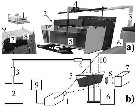
Figure 4.
Experimental setup. (a) Photograph, (b) Scheme. The components of the setup are: (1) Laser head, (2) distilled water tank (inlet), (3) pipeline with water flow meter, (4) tracer addition point, (5) tundish physical model, (6) residual water tank (outlet), (7) camera, (8) optical filter (wavelength of 570 nm), (9) laser source, and (10) measurement plane.
A discretization of the measurement plane was created in small areas, resulting in a uniform mesh of squares using MATLAB® 2023b (Apple Hill Drive 1 Natick, MA 01760-2098, USA), where local calibration can be performed at each square. The actual measurement plane inside the tundish was discretized into a mesh of 400 × 100 elements, resulting in an element size of 2.7 × 2.7 mm.
To measure the instantaneous concentration contours during tracer mixing, 3 mL of Rhodamine WT is injected at a concentration of 0.12 ppb through the shroud using a syringe. The camera captures images with a frequency of 30 frames per second, and we process the images every 0.25 s to follow the mixing evolution of the injected solute at the measurement plane. Every shot is post-processed using the XnConvert V1.106.0 software (Rue René de Chateaubriand 10 La neuvilette, Reims 51100 France), and a MATLAB® 2023b code is employed to convert the measured fluorescence signal into a concentration value via the local calibration curve. By using this procedure, concentration maps were obtained at different times.
3. Results and Discussion
3.1. Validation of the Fluid Flow Obtained by the Mathematical Model with Experimental Measurements
To ensure the robustness of the mathematical model for predicting the fluid flow field, a first validation was performed using the experimental data reported by Dong-Yuan Sheng [20]. Our modeling strategy consisted of meshing, turbulence model selection, and spatial discretization strategy. We compared our refined model’s results with the best-known experimental benchmark for tundishes [20,21]. The mathematical model described before was used to simulate the reported results of an experimental physical model of a single-strand tundish, without flow modifiers [21], by changing the appropriate boundary conditions and geometry. This tundish geometry was selected because it represents a well-documented and simplified reference case, allowing for the assessment of the model’s performance under controlled conditions. Although it differs from the main geometry of this study, it serves as a useful preliminary step to verify the numerical setup and turbulence model before applying them to the more complex case. Still, this first validation has the purpose of warranting our model’s capacity to describe the flow field of any tundish accurately. Sheng et al. [20] performed CFD simulations of the experimental results shown in Figure 5a. They used different modeling parameters, such as mesh size and turbulence model. Their modeling results show that predicted flow patterns in the tundish can vary considerably, even for simple single-phase flow, by changing a single modeling parameter. This highlights the risk of error associated with selecting a defined modeling practice without reliable experimental results for parameter fine-tuning. Following this strategy, we adjusted the mesh size and selected the turbulence model. The following turbulence models are available in Fluent: k-ε, k-ω, and Large Eddy Simulation (LES), among others. LES is computationally expensive for modeling the whole tundish. Therefore, we selected the realizable k-ε turbulence model. It provided profile results very close to the experimental reference and comparable to the best case selected by Sheng et al. [20].
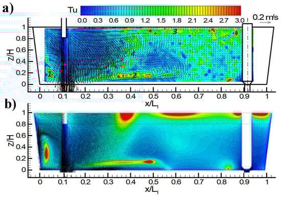
Figure 5.
Comparison of experimental velocity field and Tu [21] (a) against simulated velocity field and Tu (b).
Figure 5 compares the experimental velocity vectors and the turbulence intensity () contours against our predictions from this work’s mathematical model. Turbulence intensity is calculated using Equation (22) and is defined in the paper as the ratio of fluctuating velocity to instantaneous velocity. Vectors represent the velocities, and the model predicts the same velocities in the entering jet region, in both Figure 5a,b, for both experimental and theoretical results. When the jet impinges on the tundish bottom, it changes direction and spreads along all the directions. In the measurement longitudinal plane, one part of the jet moves laterally to the left of the jet, ascending through the wall and being redirected, forming a recirculation loop (with high turbulence characterized by a high , given by the color contour plot) and a descending diagonal flow to the right of the jet. Meanwhile, at the right side of the jet at the bottom wall, part of the fluid moves to the tundish exit, but part of it interacts with the diagonal flow and forms a high-turbulence recirculation region near the bottom center of the tundish. Part of the fluid ascends and forms a high-turbulence region near the tundish free surface. As we can see, the velocity vectors and the Tu contours show reasonable qualitative and quantitative agreement between experimental measurements and simulated results from our mathematical model.
The axial profile of the experimental [20] time-averaged velocity () at x/L = 0.5 is compared with the predicted profile from the developed model in Figure 6. The mathematical model accurately predicts the measured velocity profile with a mean relative error of 20.77 ± 20.73%. This confirms the robustness of the model to calculate tundish fluid flow. Near the free surface, small discrepancies exist between predictions and measurements. Near the bottom wall, even smaller discrepancies are observed. These results suggest that deformation of the free surface needs to be accounted for in the next model version. The current model uses a flat, fixed free surface to reduce computational cost and avoid multiphase methods like VOF. While this limits how we capture dynamic surface effects, validation shows that the model still gives reasonably accurate predictions without a deformable surface. Additionally, treatment of the walls should be fine-tuned by improving the description of the laminar-to-turbulent connection. Currently, the standard wall functions are used, but it may be necessary to consider alternative wall functions or set specific values for shear stresses or wall surface roughness.
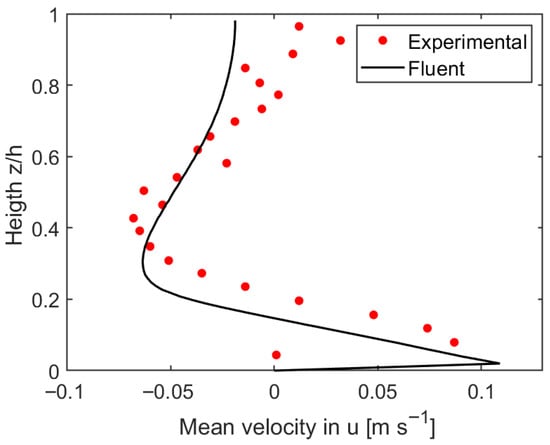
Figure 6.
Measured [20] and predicted axial profile of the time-averaged velocity of the tundish at x/L = 0.5.
Once our model’s mathematical approach, including the turbulence model and the discretization, was validated, we proceeded to simulate the fluid flow within the tundish shown in Figure 3. The purpose was to obtain the operating velocity fields in the planes indicated in Figure 3 and compare them with the experimental results obtained by PIV.
Figure 7 and Figure 8 present the tundish velocity vector fields, without flow modifiers, for three longitudinal and two transverse planes, respectively. These planes are described in Figure 3 and Table 3. On the left side, experimental velocity measurements obtained using PIV are presented; on the right side, the calculated velocity vectors derived from the mathematical model are presented. In general terms, the mathematical model properly captures the qualitative behavior of the fluid flow measured by PIV in the physical model (Figure 7 and Figure 8), considering that the experimental measurements show some fluctuations and errors due to the optical nature of the PIV measurements and the appearance of some physical interferences and optical aberrations. For instance, the mathematical model results exhibit perfect symmetric behavior due to the assumption of symmetric planes, whereas the experimental measurements reveal some asymmetries resulting from the inherent experimental error. Additionally, the mathematical model’s predicted velocity magnitude is overestimated in certain regions, particularly due to the numerical simulation’s inaccurate representation of the wall interaction with the fluid at the bottom wall.
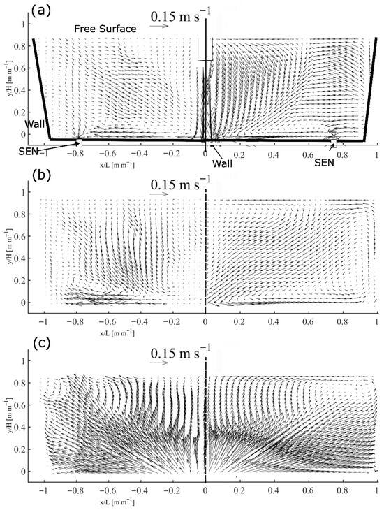
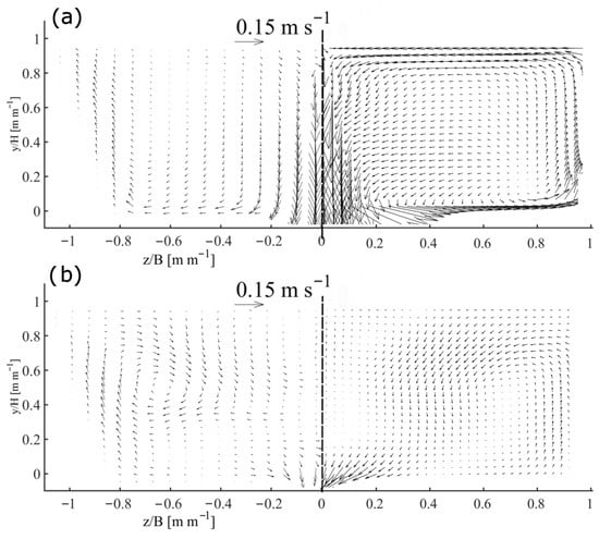
In Figure 7a, the measured and predicted velocity vector fields are shown at the middle longitudinal plane (xy) of the tundish (plane 1, xy at z = 0). We can see that in both physical and mathematical models, the jet is located just at the exit of the shroud. The jet impinges on the tundish bottom and is then redirected radially in all directions. In Figure 7a, the jet is redirected to the tundish exit; however, part of the flow ascends through the wall and is then redirected diagonally to the water jet, generating a recirculation loop. On the other hand, in Figure 8a (plane 4, middle transversal plane yz at x = 0), the flow field indicates that the water is redirected to the lateral wall, then ascends through the wall and generates a recirculation that reincorporates the flow into the jet. In both the measured and calculated flow fields, the recirculation loops in measurement planes 1 and 4 (see Figure 3) are qualitatively similar; the numerical model accurately predicts the path that the liquid follows within the tundish. The main difference lies in the quantitative value of the magnitude of the velocity vectors. The numerical simulation predicts higher velocities in general. Experimentally, the effect of the static walls on the fluid velocity is greater, slowing down the water flow as it approaches the bottom and lateral walls.
Due to the tridimensional nature of the fluid flow inside the tundish, we decided to measure the fluid dynamics of the physical model with PIV in additional measurement planes (planes 2, 3, and 5 in Figure 3), to carry out a more rigorous validation of the fluid flow predicted by the mathematical model. In Figure 7b (plane 2, xy at z = 0.6m), in general terms, it shows a projection of Figure 7a, as we can see the main movement of the water flow is the same due to the jet after interacting with the tundish bottom wall, but with a lower-velocity magnitude. In Figure 7b, the water at the bottom flows towards the lateral wall and then rises, generating a diagonal circulation loop similar to that in Figure 7a. However, there is no perceptible interaction with the tundish exit in this case. Due to the distance to the jet, a decrease in velocity magnitude in this plane is perceptible compared with the middle plane presented in Figure 7a. As in the middle plane, there is greater interaction with the walls in the measured velocities in comparison with those calculated by the simulation. In plane 3 (xy plane at z = 0.12 m), Figure 7c, as the flow approaches the tundish wall, we measure and simulate a diagonally ascending flow from the center of the tundish to the higher region of the lateral wall. This plane is interesting because the measurement showed higher velocities and was in an opposite direction from the flow patterns measured in the other two longitudinal planes (Figure 7a,b). This behavior is explained by considering the three-dimensional nature of the flow. Plane 3 shows an ascending movement of the water in the circulation loop, as shown in Figure 8a. The numerical model (Figure 7c) accurately captures the measurement’s qualitative and quantitative behavior. With a high-velocity ascending flow in a diagonal direction, some of the vectors are directed towards the tundish surface, and part of them interact with the wall, forming a circulation loop near the free surface.
Figure 8b (transverse plane yz at x = 0.44 m) shows a flow field with completely different behavior compared to Figure 8a. The jet radial movement is not perceptible in this transversal plane located away from the fluid inlet; however, circulation loops are captured in both the physical and the numerical models, and the position and magnitude of the loops are similar in both cases. These circulation loops are not generated due to the interaction of the jet movement in this plane; in this case, they are caused by the projections of the three-dimensional circulation loops shown in the middle planes (measurement planes 1 and 4 in Figure 3). As is presented in Table 4, the relative error in the mean velocity magnitudes increases (15–68%) as the measurement plane moves from the symmetry (water inlet longitudinal plane) and moves closer to the walls (planes 1–3, see Figure 3). In the transversal planes (planes 4 and 5, see Figure 3), the overprediction of the velocity magnitude by the numerical simulation is even higher (93–139%). These discrepancies suggest limitations in the turbulence model used. The system under study exhibits both high- and low-velocity regions, making it difficult for the available RANS turbulence models to accurately capture the full range of flow behavior in all planes, especially the secondary flow patterns. The increased errors near the walls may suggest additional issues with the wall function implementation. In addition, the assumption of a flat free surface is preventing the model from properly dissipating energy through the surface deformation and wave motion, as occurs in reality, contributing to the deviation between numerical and experimental results.
Table 4.
Comparison between experimental and numerical simulation of mean velocity values.
In summary, the mathematical model is capable of predicting the flow pattern in agreement with the measured flow fields, although the comparison of the predictions against the PIV experimental measurement indicates some model limitations and areas of opportunity to improve it. The main need is to improve the model’s capability to capture the water/wall interactions and also the deformable free surface.
3.2. Validation of the Predicted Mixing by the Mathematical Model with PLIF Measurements
To verify the accuracy of the mathematical model in calculating mixing inside the tundish, PLIF measurements were compared with the simulation results of Rhodamine mixing behavior. Figure 9 presents the instantaneous concentration contours measured using PLIF (left) and numerically simulated (right) at different times after the tracer was pulsed injected.
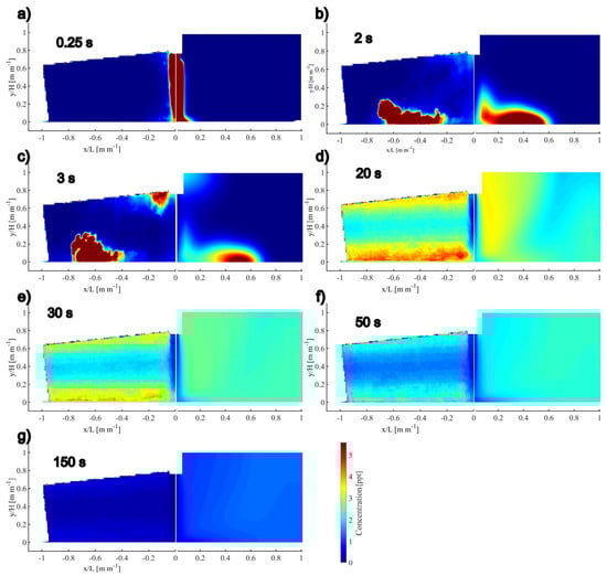
Figure 9.
Instantaneous experimental concentration contours (left) and predicted by the model concentration contours (right), obtained at (a) 0.25 s, (b) 2 s, (c) 3 s, (d) 20 s, (e) 30 s, (f) 50 s, and (g) 150 s.
Figure 9a shows the instantaneous concentration contours at 0.25 s. In both cases, the tracer follows the flow pattern depicted in Figure 7a. After injection, the Rhodamine is transported by the water jet to the tundish bottom. The mathematical model indicates that the tracer has already reached the bottom, whereas the experimental measurement suggests that the tracer is approaching the tundish bottom.
After two seconds from injection (Figure 7b), most of the tracer is moving as a high-concentration fluid package, transported by convection, following the flow pattern presented in plane 1 (Figure 7a). The experimental concentration contour shows more tracer displacement, practically reaching the tundish exit, and with a very low quantity of tracer in the jet region. At the same time, the mathematical model predicts that part of the tracer is still on the jet, showing a gradient of concentration from the jet end to the tundish exit. The PLIF measurement also shows some lateral dispersion of the tracer due to the turbulent diffusion in the jet surroundings. On the other hand, the mathematical model predicts a slight lateral dispersion due to turbulent diffusion near the main tracer package. Both convective and turbulent diffusion species transport mechanisms are underestimated in the mathematical model relative to the PLIF measurements.
Figure 9c shows that after 3 s, in both the measured and the simulated concentration contours, part of the tracer is leaving the tundish, while a region of high concentration of Rhodamine can be observed near the shroud. This region is due to the three-dimensional nature of the tundish flow, as part of the tracer follows the flow pattern presented in plane 4 (Figure 8a) and is recirculated, hence being visible on measurement plane 1 (see Figure 3). The concentration in the experimental measurement is higher and exhibits a larger and more chaotic lateral dispersion, which reinforces the notion that the mathematical model underestimates the species transport mechanisms.
Figure 9d shows that after 20 s, the tracer is more evenly distributed inside the tundish with a region with zero concentration at the water jet. The mathematical model predicts a concentration gradient from the jet to the lateral wall. However, the experimental measurement shows two bands of high concentration at the surface and the bottom of the tundish. This phenomenon is attributed to an error due to the optical nature of the PLIF technique, specifically the luminosity gradient in the laser sheet [17]. Regardless of this, the concentration values in both models are nearly the same, from 2 to 3.5 ppt. After 30 and 50 s (Figure 9e,f), the tracer is more evenly distributed in the tundish, and the concentration is decreasing to about 3 ppt and 2.5 ppt, respectively. The gradient of concentration due to the PLIF non-homogeneous illumination is still visible. Finally, at 150 s (Figure 9g), the concentration of rhodamine inside the tundish is negligible in both the experimental measurements and the mathematical model, with values below 1.5 ppt. The values of mean concentration at every time are presented at Table 5.
Table 5.
Comparison between experimental and predicted numerical values of mean concentration of rhodamine.
Table 5 shows that, except at 0.25 s and 150 s, the errors of the numerical model are generally moderate (most around 20%). At 0.25 s, the large error likely results from the actual injection point being just before the inlet, causing the solute to enter the tundish after a brief travel and pre-mixing, instead of a true pulse at the precise inlet. At 150 s, the solute is highly diluted, and the error, which is relative to the measured values, increases as the rhodamine concentration decreases to a measured value below 1 ppt.
Nevertheless, we still think the mathematical model predicts reasonably well the fluid flow of the tundish (see Figure 7 and Figure 8), and the mixing of the Rhodamine is also properly captured by the model (see Figure 9) according to the PIV and PLIF measurements. The transport of the tracer by convection following the flow pattern of the tundish is qualitatively well calculated by the numerical model, as well as the description of the lateral dispersion due to the turbulent diffusion. However, the use of PLIF measurements through instantaneous concentration contours to validate the tracer distribution predicted by the model presents some areas of opportunity to quantitatively improve the calculation of species transport mechanisms in the mathematical model, mainly the turbulent diffusion that has a greater significance in the physical model than in the mathematical model, but also the convective transport of the tracer, which is slightly underestimated in the mathematical model.
To quantify the effect of the mass transport mechanisms on the mixing inside the tundish, the instantaneous convection and instantaneous turbulent diffusion mass transfer flux were calculated with the formulation described in [22].
To further investigate the mass transfer physics, Figure 10 presents the comparison of experimental and numerical simulated instantaneous (at time of 2 s after tracer injection) convective flux, turbulent diffusion flux, and the ratio between both mass transfer mechanisms () calculated as (Equation (23)):
where and are the instantaneous convective flux and instantaneous turbulent diffusive flux, respectively.
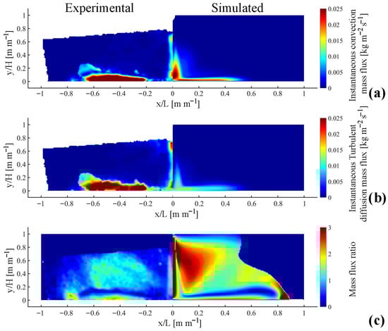
Figure 10.
Experimental (left) and numerical simulated (right); (a) instantaneous convective flux, (b) instantaneous turbulent diffusive flux, and (c) mass flux ratio at 2 s after the tracer injection.
Figure 10a,b present a similar distribution of the instantaneous mass transfer mechanisms, where a high convective and turbulent diffusive flux at the jet and at the lateral region after the tracer impinges with the tundish bottom, presenting high flux values at the regions where the tracer concentration is high (see Figure 9b). In both experimental and simulated flux results, the convective flux (Figure 10a) presents a higher value compared with the turbulent diffusive flux (Figure 10b). Table 6 presents the mean value of the mass transfer fluxes in measurement plane 1 (see Figure 3). The mean convection flux is 21% and 57% higher compared with the turbulent diffusion flux (only considering the mean value of the mechanism in the plane) for experimental and numerical simulation, respectively. We can also observe that the numerical simulation yields significantly lower values in both mass fluxes, with the experiment presenting 3.6 times and 4.7 times more convection and turbulent diffusion mass flux, respectively.
Table 6.
Mass transfer fluxes mean values at the measurement plane 1 (see Figure 3).
To explore the difference between the numerical values of the fluxes, the local ratio between both fluxes was calculated (see Figure 10c). Notably, the local mass flux ratio is higher in the numerical simulation (mean value 1.21) than in the experimental measurement (mean value 0.51; see Table 6). This suggests that the model does not accurately represent the relationship between velocity and turbulence, likely due to the turbulence model. However, in qualitative terms, the flux ratio is similar: in most of the tundish, convection dominates mass transport, whereas just above the bottom, turbulent diffusion dominates. Specifically, after the jet impinges on the bottom, part of the tracer is transported to the tundish exit by convection. Subsequently, a region above this forms a layer where turbulent diffusion becomes the dominant mechanism.
4. Conclusions
Advanced experimental tools, such as PIV and PLIF, helped select the realizable k-ε turbulence model. This model could predict the main features in several transverse and longitudinal planes. It did so both qualitatively and quantitatively for fluid flow patterns, turbulence, and solute mixing in a physical two-strand tundish model. Using these techniques for verification and validation of mathematical models in metallurgical continuous systems, or similar systems, has proven to be the most effective analysis route in metallurgical process engineering.
The mixing phenomena of a tracer are described by mass transfer mechanisms: convection, turbulent diffusion, and turbulent dispersion. Therefore, a model must properly describe the time-averaged flow field and the fluctuations of velocity (turbulence) to predict tracer mixing.
In conclusion, addressing these limitations is essential to significantly enhancing the predictive accuracy of the model. Improving the representation of wall–fluid interaction and free surface deformation, as well as refining turbulence modeling, will reduce the relative errors in velocity and chemical composition, currently at 15% to 94% and around 20%, respectively, and provide a more robust basis for future simulation work.
Author Contributions
Conceptualization, A.M.A.-V. and M.A.R.-A.; Investigation, C.G.-R.; Methodology, A.V.-S. and L.E.J.-P.; Resources, M.A.R.-A.; Supervision, M.A.R.-A.; Validation, A.M.A.-V.; Writing—original draft A.V.-S.; Writing—review and editing, L.E.J.-P., C.G.-R. and M.A.R.-A. All authors have read and agreed to the published version of the manuscript.
Funding
This research received no external funding.
Data Availability Statement
The original contributions presented in this study are included in the article. Further inquiries can be directed to the corresponding author.
Acknowledgments
Alberto Velázquez-Sánchez, CVU 915275, as a student registered in the Doctoral Program in Chemical Engineering at the Universidad Nacional Autónoma de México (UNAM), thanks SECIHTI for the financial support through a Ph.D. scholarship.
Conflicts of Interest
The authors declare no conflicts of interest.
References
- Mazumdar, D.; Guthrie, R.I.L. The Physical and Mathematical Modelling of Continuous Casting Tundish Systems. ISIJ Int. 1999, 39, 524. [Google Scholar] [CrossRef]
- Chattopadhyay, K.; Isac, M.; Guthrie, R.I. Physical and Mathematical Modelling of Steelmaking Tundish Operations: A Review of the Last Decade (1999–2009). ISIJ Int. 2010, 50, 331–348. [Google Scholar] [CrossRef]
- Mazumdar, D. Review, Analysis, and Modeling of Continuous Casting Tundish Systems. Steel Res. Int. 2019, 90, 1800279. [Google Scholar] [CrossRef]
- Rajasekar, K.; Kumar, A. Effect of Flow Modifiers on the Fluid Flow Characteristics in a Slab Caster Tundish. CA. Metall. Q. 2025, 64, 1724–1739. [Google Scholar] [CrossRef]
- Yue, Q.; Li, Y.; Wang, Z.M.; Sun, B.C.; Wang, X.Z. Analysis Model of Internal Residence Time Distribution for Fluid Flow in a Multi-Strand Continuous Casting Tundish. J. Iron Steel Res. Int. 2024, 31, 2186–2195. [Google Scholar] [CrossRef]
- Constantino, M.; Barreto, J.d.J.; Garcia-Hernandez, S.; Gutierrez, E.; Constantino, A.; Venegas-Rebollar, V. Analogous Water Modeling of an Asymmetric Multiple Strand Tundish Using Turbulence Inhibitors and Bubble Diffusers. ISIJ Int. 2025, 65, 417–425. [Google Scholar] [CrossRef]
- Maurya, A.; Singh, P.K. Effect of Ladle Shroud Design on Tundish Hydrodynamic Performance and Attendant Influence on Tundish Open Eye. Steel Res. Int. 2025, 2500081. [Google Scholar] [CrossRef]
- Zhang, L.; Gu, S.; Wang, H.; Li, T.; Tan, M.; Liu, K.; Tang, G. Multiphase Modeling of Inclusion Removal by Bubble Adhesion in the Submerged Entry Nozzle with Centrifugal Swirling Flow. Ironmak. Steelmak. 2025, 52, 66–84. [Google Scholar] [CrossRef]
- Sheng, D.Y. Thermal Analysis of Continuous Casting Tundish Using a Conjugate Heat Transfer Model. JOM 2025, 77, 4019–4026. [Google Scholar] [CrossRef]
- Demeter, P.; Buľko, B.; Dzurňák, R.; Priesol, I.; Hubatka, S.; Fogaraš, L.; Demeter, J. The Development of an Optimized Impact Pad for a Six-Strand Tundish Using CFD Simulations. Appl. Sci. 2025, 15, 5450. [Google Scholar] [CrossRef]
- Dinda, S.K.; Li, D.; Guerra, F.; Cathcart, C.; Barati, M. Continuous Casting Tundish Dead Volume Study by Physical Modeling and Computational Investigation. Steel Res. Int. 2024, 95, 2400125. [Google Scholar] [CrossRef]
- Geng, M.; Wang, T.; Chen, C. Assessment of the Volume Effect and Application of an Improved Tracer in Physical Model of a Single-Strand Bare Tundish. Metall. Mater. Trans. B 2024, 55, 4121–4131. [Google Scholar] [CrossRef]
- Li, D.; Duan, H.; Chen, W.; Zhang, L. Deriving Tundish Flow Fields through Ink Diffusion Experiments Based on Image Processing. Metall. Mater. Trans. B 2025, 56, 4742–4753. [Google Scholar] [CrossRef]
- Koitzsch, R.; Odenthal, H.J.; Pfeifer, H. Concentration Measurements in a Water Model Tundish using the Combined DPIV/PLIF Technique. Steel Res. Int. 2007, 78, 473. [Google Scholar] [CrossRef]
- Braun, A.; Pfeifer, H. Mehrphasenströmung in der Metallurgie – Vergleich CFD-Simulation mit PLIF-Messungen. In Proceedings of the Symposium zur Simulation metallurgischer Strömungen an österreichischen und deutschen Universitäten, Rostock, Germany, 1–4 March 2006. [Google Scholar]
- Cwudzinski, A.; Jowsa, J.; Gajda, B. Physical Modelling of Fluids’ Interaction during Liquid Steel Alloying by Pulse-Step Method in the Continuous Casting Slab Tundish. Ironmak. Steelmak. 2020, 47, 1188. [Google Scholar] [CrossRef]
- Velázquez-Sánchez, A.; Jardón-Pérez, L.E.; Villarreal-Medina, R.; González-Rivera, C.; Amaro-Villeda, A.M.; Ramírez Argáez, M.A. Advantage of utilizing PLIF to Analyze Mixing Phenomena in a Physical Model of a Two-strand Continuous Casting Tundish. JOM 2025. [Google Scholar] [CrossRef]
- Hua, C.; Wang, D.; Guan, J.; Zhang, H.; Hu, X.; Ren, Z.; Li, Y. Particle Image Velocimetry Measurements and Numerical Simulation of the Flow and Vortex in a Hydraulic Mountain-Bottom Submerged Entry Nozzle. Steel Res. Int. 2025, 96, 2400893. [Google Scholar] [CrossRef]
- Zhang, Z.; Qu, T.; Wang, D.; Li, X.; Fan, L.; Zhou, X. Non-Uniform Thermal Transfer of Molten Steel and Its Effect on Inclusion Particles Removal Behavior in Continuous Casting Tundish. Metals 2025, 15, 170. [Google Scholar] [CrossRef]
- Sheng, D.Y. Synthesis of a CFD Benchmark Exercise: Examining Fluid Flow and Residence-Time Distribution in a Water Model of Tundish. Materials 2021, 14, 5453. [Google Scholar] [CrossRef]
- Odenthal, H.J.; Mirko, J.; Marcus, K.; Norbert, V. CFD benchmark for a single strand tundish (Part I). Steel Res. Int. 2010, 80, 264–274. [Google Scholar] [CrossRef]
- Jardón-Pérez, L.E.; González-Rivera, C.; Trápaga-Matrínez, G.; Amaro-Villeda, A.M.; Ramírez Argáez, M.A. Experimental Study of Mass Transfer Mechanisms for Solute Mixing in a Gas-Stirred Ladle using the Particle Image Velocimetry and Planar Laser-Induced Fluorescence Techniques. Steel Res. Int. 2021, 92, 2100241. [Google Scholar] [CrossRef]
Disclaimer/Publisher’s Note: The statements, opinions and data contained in all publications are solely those of the individual author(s) and contributor(s) and not of MDPI and/or the editor(s). MDPI and/or the editor(s) disclaim responsibility for any injury to people or property resulting from any ideas, methods, instructions or products referred to in the content. |
© 2025 by the authors. Licensee MDPI, Basel, Switzerland. This article is an open access article distributed under the terms and conditions of the Creative Commons Attribution (CC BY) license (https://creativecommons.org/licenses/by/4.0/).