Abstract
The influencing factors of wax deposition are numerous and complex, and accurately predicting the wax deposition rate is of great practical significance for the safe operation of pipelines and the formulation of reasonable pigging schemes. On the basis of mastering the prediction steps of the Elman neural network (ENN), the arithmetic optimization algorithm (AOA) was introduced to improve the Elman neural network and an optimization model was established, and the differences in prediction results between improved models (AOA-ENN model, PSO-ENN model, GA-ENN model) and the traditional ENN model were compared and analyzed through examples. The prediction results of three examples showed that the average relative errors of the AOA-ENN model are 2.5470%, 1.4974%, and 2.3819 %, respectively, while the average relative errors of the traditional ENN model are 19.0313%, 9.1568%, and 11.4836%, respectively. Therefore, the arithmetic optimization algorithm used in this paper has good reliability. For the three improved models, the AOA-ENN model has the highest prediction accuracy, followed by the PSO-ENN model and the GA-ENN model. Overall, the Elman neural network improved by an arithmetic optimization algorithm can be used for predicting wax deposition rate, which can provide new ideas for accurate prediction of wax deposition rate.
1. Introduction
During the pipeline transportation of waxy crude oil, when the oil temperature is lower than wax appearance temperature of the crude oil, the wax crystals begin to precipitate in the oil flow and eventually deposit on the pipe wall [1,2]. Wax deposit sediment can reduce the flow area of pipelines, reduce their conveying capacity and lead to pipeline blockage in severe cases [3,4,5]. The phenomenon of wax deposition seriously affects the safe operation of pipelines and can bring huge economic losses [6,7]. Therefore, the urgency and necessity of studying and solving the problem of wax deposition are becoming increasingly prominent [8].
In order to ensure the safe operation of pipelines, it is necessary to grasp the distribution rule of wax deposition rate or deposition thickness of pipelines. For the study of wax deposition rate or thickness, experimental simulation methods can be used. Currently, the commonly used experimental devices include cold finger and loop devices [9,10,11]. The operation of the cold finger experimental device is simple, but the flow state of the fluid in the device differs greatly from the actual pipeline flow [12]. The loop experimental device can simulate actual pipe flow more realistically, so it has been widely used. As is well known, wax deposition experiments generally require a lot of time and manpower, which makes the data obtained by researchers from wax deposition experiments generally limited. Therefore, it is particularly important to establish reliable methods and models for predicting wax deposition rate using the obtained experimental data. Based on the prediction methods and models, the wax deposition rate can be obtained quickly, which has the advantages of reducing the number of experiments and facilitating the acquisition of wax deposition rate.
Huang et al. established a universal wax deposition model by considering the main influencing factors of wax deposition and conducting relevant theoretical analysis. The results showed that the average error of the model is 6.32%, and the maximum error is 20% [13]. Peng established a dynamic prediction model suitable for calculating the wax deposition thickness, and the results showed that the model can predict the wax deposition process more accurately [14]. Singh et al. established a model that can predict the growth of wax deposition layer thickness and wax content in the deposition layer. The authors pointed out that the wax molecules will further diffuse into the sedimentary layer when they diffuse to the surface of the sedimentary layer, and the oil molecules in the sedimentary layer will reverse diffuse from the sedimentary layer to the oil flow, thus increasing the wax content in the sedimentary layer [15]. Based on this mechanism, Huang applied it to predict the amount of wax deposition and the wax content in the sedimentary layer, and achieved good prediction results [16]. Farimanii et al. considered the influence of wax crystal precipitation kinetics in the boundary layer on wax deposition and established a wax deposition model. The authors pointed out that this model can achieve relatively good prediction results [17].
In addition to using theoretical models to predict wax deposition rate or thickness, the machine learning methods to predict wax deposition rate is also an effective measure. Obanijesu and Omidiora used the artificial neural network method to predict the wax deposition in the reservoir, and the results showed that the prediction results are in good agreement with the actual data [18]. Xie and Xing used RBF neural network to predict the wax deposition rate based on indoor wax deposition experimental data, and achieved good results [19]. Chu et al. used the PSO method to optimize the parameters of the ANFIS model and predicted the wax deposition amount. The authors pointed out that the prediction accuracy of the constructed model was higher than that of previous models [20]. Dehaghani developed an ANN model to predict the thickness of wax deposition, and the results indicated that the predicted values obtained by the ANN model are relatively close to the experimental results [21]. Eghtedaei et al. used radial basis function neural network to predict wax deposition, and the results showed that an RBF-ANN model can achieve good prediction results [22]. Jalalnezhad and Kamali predicted the wax deposition thickness under single-phase turbulence using an adaptive neuro fuzzy inference system, and the research results showed that this method has a good prediction effect [23]. Based on the experimental results, Amar et al. introduced the Levenberg–Marquardt algorithm to optimize the multilayer perceptron (MLP), and proposed an intelligent method (MLP-LMA) to predict the wax deposition problem. The results showed that the performance of MLP-LMA is better, and the total root mean square error is 0.2198 [24]. Ramsheh et al. developed a new intelligent model to predict wax deposition by combining cascade forward and generalized regression neural network (GRNN). The results showed that the GRNN model has a good prediction effect on wax deposition, and the root mean square error is 0.845 [25].
In the process of neural network prediction, the Elman neural network is a typical dynamic artificial neural network that has been widely applied in multiple fields. Compared with ordinary neural networks, Elman neural network has a special receiving layer that enables them to have unique dynamic characteristics [26]. Like some neural networks, the Elman neural network also used gradient descent method in its application, which easily leads to slow training speed and falling into local minima [26]. An arithmetic optimization algorithm is a new method proposed by Abualigah et al. in 2021, which has the advantages of no complex parameter adjustment and a fast rate of convergence [27,28].
Based on this, this article used arithmetic optimization algorithms to improve the Elman neural network and established an AOA-ENN model to predict the wax deposition rate of waxy crude oil. In addition, the differences in prediction accuracy between the improved models (AOA-ENN model, PSO-ENN model, and GA-ENN model) and the traditional model were compared and analyzed. The research results can provide useful reference for accurate prediction of wax deposition rate.
2. Basic Theory of Elman Neural Network and Arithmetic Optimization Algorithm
2.1. Elman Neural Network (ENN)
The Elman neural network is generally divided into four layers: input layer, hidden layer, context layer, and output layer, as shown in Figure 1 [29].
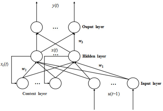
Figure 1.
The network structure of ENN.
The structural expression of Elman neural network is as follows [29,30]:
For the operating principle of Elman neural network, many studies have provided detailed introductions, and readers can refer to the literature [26] for more details.
2.2. Arithmetic Optimization Algorithm (AOA)
The arithmetic optimization algorithm uses the rule of four arithmetic operations to achieve global optimization. The optimization strategy is selected through the math optimizer accelerated function, that is, multiplication and division are used for global search, and addition and subtraction are used for local exploitation. The specific implementation principle is as follows [27,31,32]:
- (1)
- Initialization phase
Based on Equation (4), the random numbers are generated to complete the initialization of the population.
Before optimization, the specific function values of the math optimizer accelerated based on Equation (5) are obtained, and the final decision is made based on the function values (exploration phase or exploitation phase).
- (2)
- Exploration phase
The operators at this stage are multiplication (M) and division (D), which have high dispersion. The specific mathematical model is
MOP is the math optimizer probability (a coefficient), and it can be calculated by using Equation (7).
- (3)
- Exploitation phase
The operators in this stage are addition (A) and subtraction (S), which have significant low dispersion. The specific mathematical model is
The parameters (μ) generate non identical random values in each iteration to ensure continuous exploitation, which is beneficial for jumping out of local optimal and finding global optimal solution.
3. The Steps for Predicting Wax Deposition Rate Using Elman Neural Network and Improved Elman Neural Network
3.1. The Prediction Steps of Elman Neural Network
Based on the test results of wax deposition rate, Elman neural network is used to predict the wax deposition rate. The specific steps are as follows:
Step 1: The influencing factors of wax deposition rate as input data and the wax deposition rate as output data. Some data are randomly selected from the wax deposition test results as training samples, and the remaining data as prediction samples;
Step 2: The data are normalized (the mapminmax function is used);
Step 3: The structure of the Elman neural network model is determined;
Step 4: The weight values and threshold values are randomly initialized;
Step 5: The fitness values are calculated, and the final threshold values and weight values are determined. Among them, f(.) is the Sigmoid function and g(.) is the linear function;
Step 6: Prediction results are output and model prediction accuracy are analyzed.
3.2. The Prediction Steps of Improved Elman Neural Network
The arithmetic optimization algorithm is used to improve the Elman neural network, and the specific flow chart is shown in Figure 2. Based on the flow chart and combined with Python programming language (version number: 3.12.5), the prediction results of wax deposition rate can be obtained.
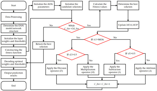
Figure 2.
The flow chart of improved ENN model.
The specific steps are as follows:
Step 1: Firstly, the measured data of wax deposition rate of crude oil pipeline are normalized, and then the traditional ENN model is initialized and the numbers of various layers of network structure are determined. In addition, the population size, spatial dimension and other parameters of the arithmetic optimization algorithm are initialized.
Step 2: Initializing the population of the arithmetic optimization algorithm, and calculating the initial fitness value (Mean squared error of training samples is used).
Step 3: The iterative steps are executed, and Equations (7) and (5) are used to update MOP and MOA, respectively; if r1 > MOA, the global exploration phase will be entered and the position is updated according to Equation (6); otherwise, the local exploitation phase will be entered and the position is updated according to formula (8); comparing the fitness value of the current position with the fitness value of the current optimal position, and if the fitness value of the current position is better, then the fitness value will be updated. Otherwise, it will not be updated.
Step 4: Determining whether the maximum number of iterations has been reached. If the maximum number of iterations is reached, then the final optimal fitness value (the optimal threshold values and weight values of the Elman neural network) is output and the loop is terminated. Otherwise, return to step 3.
Step 5: The optimal solution (the optimal weight values and threshold values) obtained by arithmetic optimization algorithm is assigned to the ENN model, then an improved ENN model is obtained through matrix reconstruction, and the wax deposition rate of waxy crude oil is predicted.
4. Comparison and Accuracy Analysis of Model Prediction Results
4.1. Comparison of Prediction Results for Wax Deposition Rate (Example 1)
The author of reference [33] provided experimental data of wax deposition rate under different influencing factors. Of the total 37 sets of data, 32 sets of data were randomly selected as training samples and the remaining 5 sets of data as prediction samples (as shown in Table 1).

Table 1.
Predicted samples (Example 1).
Before the prediction, the network structure of the ENN model should be determined. In order to obtain the structure of the ENN model, it is important to determine the number of hidden layer nodes. The steps to determine the optimal number of hidden layer nodes are summarized as follows:
Step 1: The value range of the number of hidden layer nodes is determined based on the empirical Formula (10).
Step 2: The mean square errors of training samples with different number of hidden layer nodes are calculated.
Step 3: When the mean square error is the smallest, the corresponding number of hidden layer nodes is the optimal number of hidden layer nodes.
According to the above steps, the mean square errors of training samples with different number of hidden layer nodes are calculated (Table 2).
Table 2.
Mean square error of training samples for each hidden layer node (Example 1).
According to the calculation results in Table 2, the optimal number of hidden layer nodes is determined (the value is 7). Therefore, the structure of ENN model is 7–7–1.
Based on the above prediction steps, the prediction results of the ENN model and the AOA-ENN model (a Elman neural network model improved by arithmetic optimization algorithm) are obtained, as shown in Table 3.
Table 3.
Prediction results and relative errors of different models (Example 1).
In the prediction process of the AOA-ENN model, the main relevant parameters used are as follows: ① The population size needs to balance the computational cost and population diversity in the selection process, and its value should not be too small or too large. After several adjustments, it is found that when the population size is 30, a good balance between computational efficiency and population diversity can be achieved, so the final population size is 30. ② The convergence and time cost should be considered in the selection of the number of iterations. Based on the convergence curve, reducing the number of iterations appropriately can avoid more time consumption (under the condition of ensuring convergence). Based on this, the number of iterations determined in this paper is 50. ③ The sensitivity parameter α controls the dynamic transition time of the algorithm from global exploration to local exploitation, and the balance between exploration and exploitation needs to be considered in the selection process. Previous studies have shown that when the value of α is 5, the algorithm can have sufficient exploration in the early stage and smoothly transition to fine exploitation in the later stage. Therefore, the sensitivity parameter determined in this paper is 5. ④ The control parameter μ is a very small constant, which is used to prevent the denominator from being zero in the division operation. In the process of selecting a control parameter, it is necessary to ensure that the generated new solution does not deviate too far from the current boundary and provides sufficient randomness (a smaller value close to 0.5 can be taken). Therefore, the control parameter used in this paper is 0.499.
In addition, in order to verify the prediction accuracy of the AOA-ENN model, this paper also uses the conventional optimization algorithm (particle swarm optimization algorithm and genetic algorithm) to improve the Elman neural network, and establishes the PSO-ENN model (Elman neural network model improved by particle swarm optimization algorithm), and the GA-ENN model (Elman neural network model improved by genetic algorithm). In the prediction process of the PSO-ENN model, the main relevant parameters used are as follows: the number of iterations is 50; the population size is 30; individual learning factor is 1.5; social learning factor is 1.5; and inertia weight is 0.8. In the prediction process of the GA-ENN model, the main relevant parameters used are as follows: the number of iterations is 50; the population size is 30; the crossover probability is 0.8 and the mutation probability is 0.2.
The measured values and the predicted values of different models are shown in Table 3 and Figure 3. In the prediction process of Example 1, the running time of the traditional ENN model, the AOA-ENN model, the PSO-ENN model, and the GA-ENN model is 5 s, 1 min 27 s, 1 min 28 s, and 1 min 36 s, respectively.
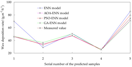
Figure 3.
Comparison of the prediction results for different models and test results (Example 1).
It can be seen from Table 3 and Figure 3 that the predicted values of the AOA-ENN model are the closest to the measured values, and the maximum relative error of the predicted results is the lowest. Compared with the ENN model, the relative errors of the AOA-ENN model, the PSO-ENN model, and the GA-ENN model are greatly reduced.
In order to further analyze the prediction accuracy of the traditional ENN model and each improved model, the average relative errors and root mean square errors of different models are calculated, as shown in Table 4.
Table 4.
Comparison of errors for different models (Example 1).
From Table 4, it is evident that the average relative error of the traditional ENN model is 19.0313%, and the root mean square error is 12.3537, so the prediction effect of ENN model is relatively poor. After using the arithmetic optimization algorithm to improve the Elman neural network, the two types of errors are greatly reduced (they are 2.5470% and 1.6166, respectively), so the AOA-ENN model has higher prediction accuracy.
For the traditional ENN model, its shortcomings in the prediction process are mainly summarized as follows: ① The network structure contains recursive connections and the training requires multiple iterations, so the time consumption is significantly increased when dealing with large-scale data; ② The gradient descent method makes it easy to fall into the local minimum value, and it is difficult to achieve the global optimal solution; ③ The prediction performance is highly dependent on the setting of parameters such as weight initialization and learning rate, and improper parameters can easily lead to convergence failure; ④ It is easy for overfitting to occur, which directly affects the generalization ability of the model.
After introducing the arithmetic optimization algorithm, the prediction accuracy of the traditional Elman neural network model can be significantly improved, and the main reasons are as follows: ① The algorithm adopts the mathematical operation search mechanism, which can efficiently traverse the optimal solution in a larger parameter space and significantly reduce the risk of local optimum; ② The algorithm can quickly locate the optimization direction of the parameters and shorten the convergence period by global exploration and local exploitation; ③ The algorithm can take the key parameters of the network (weight values, threshold values, etc.) as the optimization variables, and obtain the optimal threshold values and weight values through the optimization of the objective function; ④ The global optimization characteristic of the algorithm can reduce the over-fitting of the traditional model and enhance the generalization ability.
Comparing the average relative error and root mean square error of the each improved model, it can be seen that the prediction accuracy of the AOA-ENN model is the highest, followed by the PSO-ENN model and the GA-ENN model. In general, the prediction accuracy of the AOA-ENN model and the PSO-ENN model is higher. In the process of improving the Elman neural network, the differences between the two algorithms are mainly summarized as follows: ① Search method: AOA relies on arithmetic operations to achieve parameter search, and its search process pays more attention to the uniform traversal of parameter space; the PSO algorithm realizes search through particle velocity update, which relies more on information sharing and group collaboration between particles. ② Search characteristics: AOA has low dependence on the initial solution, and it may lead to slow convergence for high-dimensional problems; the PSO algorithm initially tends to be global exploration, and local exploitation in the later stage. In this case, it may premature convergence or fall into local optimum. ③ Computational complexity and adaptability: the computational complexity of the AOA-ENN model is more focused on the randomness of solution generation and fitness evaluation, and it is suitable for high-dimensional problems but requires more iterations; the computational complexity of the PSO-ENN model focuses on inter-particle collaboration and speed update, and it is suitable for low-dimensional optimization but may increase the total time consumption due to premature convergence.
4.2. Comparison of Prediction Results for Wax Deposition Rate (Example 2)
The author of reference [34] provided experimental data of wax deposition rate under different influencing factors (a total of 38 sets of data), the 30 sets of data were randomly selected as training samples and the remaining 8 sets of data as prediction samples (as shown in Table 5).
Table 5.
Predicted samples (Example 2).
In order to determine the number of hidden layer nodes, the mean square error of training samples for each hidden layer node are calculated (Table 6).
Table 6.
Mean square errors of training samples for each hidden layer node (Example 2).
Based on the calculation results in Table 6, the optimal number of hidden layer nodes is determined (the value is 4). Therefore, the structure of ENN model is 7–4–1.
According to the obtained model structure, the prediction results of the ENN model, AOA-ENN model, PSO-ENN model, GA-ENN model are obtained, as shown in Table 7 and Figure 4. In the prediction process of example 2, the running time of the traditional ENN model, the AOA-ENN model, the PSO-ENN model, and the GA-ENN model is 6 s, 1 min 19 s, 1 min 24 s, and 1 min 42 s, respectively. In addition, the setting of relevant main parameters are consistent with example 1 in the prediction process.
Table 7.
Prediction results and relative errors of different models (Example 2).
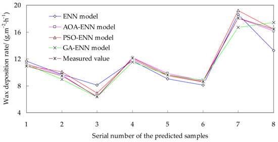
Figure 4.
Comparison of the prediction results for different models and test results (Example 2).
Similarly, the different kinds of errors for various models are further obtained, the results are shown in Table 8.
Table 8.
Comparison of errors for different models (Example 2).
It can be seen from Table 7 and Figure 4 that the maximum relative error of the predicted results for the AOA-ENN model is the lowest, and the relative error can be controlled within 4%. In addition, the relative errors of the traditional ENN models are generally higher than those of improved models (AOA-ENN model, PSO-ENN model, and the GA-ENN model).
From Table 8, it is evident that the average relative error of the ENN model is relatively large (9.1568%), so the traditional model has a large prediction deviation under multi-factor coupling conditions. After using an arithmetic optimization algorithm to improve the Elman neural network, the two types of errors are only 1.4974% and 0.1830, respectively, so the AOA-ENN model can achieve good prediction accuracy. Compared with the PSO-ENN model, and GA-ENN model, the two types of errors of the AOA-ENN model are lower. Therefore, the AOA-ENN model has higher prediction accuracy.
4.3. Comparison of Prediction Results for Wax Deposition Rate (Example 3)
In order to verify the effectiveness of the AOA-ENN model, the wax deposition data from an offshore oilfield were used for further analysis. The author of reference [35] collected the wax deposition test data from an offshore oilfield (a total of 30 sets of data), the 25 sets of data were randomly selected as training samples and the remaining 5 sets of data as prediction samples (as shown in Table 9).
Table 9.
Predicted samples (Example 3).
Based on the determination method of the number of hidden layer nodes in Example 1 and Example 2, the mean square errors of training samples for each hidden layer node are calculated, and the results are shown in Table 10.
Table 10.
Mean square errors of training samples for each hidden layer node (Example 3).
According to the calculation results in Table 10, the optimal number of hidden layer nodes can be determined (the number of hidden layer nodes is 5), so the 5–5–1 network model structure can be constructed.
Based on the determined ENN model structure, the predicted values of different models are obtained, and the predicted values are compared with the measured values (as shown in Table 11 and Figure 5). In the prediction process of Example 3, the running time of the traditional ENN model, the AOA-ENN model, the PSO-ENN model, and the GA-ENN model is 4 s, 1 min 23 s, 1 min 29 s, and 1 min 37 s, respectively. In addition, the setting of relevant main parameters are consistent with example 1 in the prediction process.
Table 11.
Prediction results and relative errors of different models (Example 3).
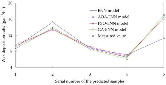
Figure 5.
Comparison of the prediction results for different models and test results (Example 3).
From Table 11 and Figure 5, it can be seen that the predicted values of the AOA-ENN model, the PSO-ENN model, and the GA-ENN model are close to the measured values, and their prediction accuracy is better. Compared with the ENN model, the relative errors of the AOA-ENN model, the PSO-ENN model, and the GA-ENN model are greatly reduced.
Similarly, the different kinds of errors for various models are calculated, and the results are shown in Table 12.
Table 12.
Comparison of errors for different models (Example 3).
From Table 12, it is evident that the average relative error of the AOA-ENN model is the lowest, followed by the PSO-ENN model and the GA-ENN model, so the AOA-ENN model has the highest prediction accuracy. Compared with each improved model, the two types of errors for the traditional ENN model are larger, and the prediction accuracy is poor.
5. Conclusions
- There are many factors affecting the wax deposition rate, and there is a complex nonlinear relationship between each factor and the wax deposition rate. The AOA-ENN model for predicting wax deposition rate was established by introducing the arithmetic optimization algorithm to improve the Elman neural network. The results showed that the prediction results of the AOA-ENN model are in good agreement with the measurement results, and the prediction accuracy is high. This research method provides a new idea for the accurate prediction of the wax deposition rate of the pipe wall.
- The prediction results of Example 1, Example 2, and Example 3 showed that the average relative errors of the AOA-ENN model are significantly lower than those of the traditional ENN model. Therefore, it is definitely feasible to use the AOA-ENN model to predict the wax deposition rate. For each improved model, the AOA-ENN model has the highest prediction accuracy, followed by the PSO-ENN model and the GA-ENN model.
- The arithmetic optimization algorithm does not need to perform complex mathematical operations on the objective function, and directly performs arithmetic operations on the function, which greatly simplifies the solution process of the optimization problem, and has the advantages of high efficiency and high precision.
Author Contributions
Conceptualization, W.J. and Z.C.; methodology, W.J. and Z.C.; software, W.J. and Z.C.; validation, W.J., K.D. and Q.Q.; formal analysis, W.J.; investigation, W.J., Z.C. and K.D.; resources, Z.R.; data curation, Z.C.; writing—original draft preparation, W.J.; writing—review and editing, Q.Q.; visualization, Z.C.; supervision, W.J.; project administration, W.J.; funding acquisition, W.J., Q.Q. and Z.R. All authors have read and agreed to the published version of the manuscript.
Funding
The authors gratefully acknowledge the financial support from the Open Fund of the National Key Laboratory of Oil and Gas Reservoir Geology and Exploitation (Southwest Petroleum University, No. PLN202322), the Doctoral Assistance Program of Xi’an Shiyou University (Xi’an Shiyou University, No. 134010009).
Data Availability Statement
The original contributions presented in this study are included in the article. Further inquiries can be directed to the corresponding authors.
Conflicts of Interest
Author Zhuo Chen was employed by the company The Second Oil Production Plant, Sinopec Northwest Oilfield Company. Author Kemin Dai was employed by the company China Petroleum Engineering & Construction Southwest Company. The remaining authors declare that the research was conducted in the absence of any commercial or financial relationships that could be construed as a potential conflict of interest.
Nomenclature
| y(t) | output vector |
| x(t) | output vector of the hidden layer |
| u(t) | input vector |
| xc(t) | output vector of the context layer |
| w1 | connection weight value from the input layer to the hidden layer |
| w2 | connection weight value from the context layer to the hidden layer |
| w3 | connection weight value from the hidden layer to the output layer |
| g(.) | transfer functions of the output layer |
| f(.) | transfer functions of the hidden layer |
| N | population quantity |
| n | the dimension of exploration space |
| xi,j | the position of the i-th solution in the j-th dimensional space |
| MOA(C_iter) | specific function value at the t-th iteration |
| MOA | an adaptive coefficient |
| C_iter | current number of iterations |
| M_iter | maximum number of iterations |
| max | maximum value of the corresponding function values of the math optimizer accelerated |
| min | minimum value of the corresponding function values of the math optimizer accelerated |
| r1, r2, r3 | a random number between [0, 1] |
| xi(C_iter + 1) | the i-th solution of the next iteration |
| xi,j(C_iter + 1) | the j-th dimension position of the i-th solution for the next iteration |
| best(xj) | the j-th dimension position of the best solution during the iteration process |
| ε | a small integer number |
| UBj | upper bound value of the j-th dimension position |
| LBj | lower bound value of the j-th dimension position |
| μ | control parameter to adjust the exploration process |
| MOP | math optimizer probability |
| MOP(C_iter) | function value at the t-th iteration |
| α | a sensitive parameter |
| dfi | model output value of the i-th sample |
| dvi | actual value of the i-th sample |
| m | the number of input layer nodes |
| l | the number of output layer nodes |
| a | an integer between 1 and 10 |
References
- Liu, Y.; Pan, C.L.; Cheng, Q.L.; Wang, B.; Wang, X.X.; Gan, Y.F. Wax deposition rate model for heat and mass coupling of piped waxy crude oil based on non-equilibrium thermodynamics. J. Dispers. Sci. Technol. 2018, 39, 259–269. [Google Scholar] [CrossRef]
- Mehrotra, A.K.; Bhat, N.V. Modeling the effect of shear stress on deposition from “waxy” mixtures under laminar flow with heat transfer. Energy Fuels 2007, 21, 1277–1286. [Google Scholar] [CrossRef]
- Oyekunle, L.; Adeyanju, O. Thermodynamic Prediction of Paraffin Wax Precipitation in Crude Oil Pipelines. Pet. Sci. Technol. 2011, 29, 208–217. [Google Scholar] [CrossRef]
- Wang, W.D.; Huang, Q.Y. Prediction for wax deposition in oil pipelines validated by field pigging. J. Energy Inst. 2014, 87, 196–207. [Google Scholar] [CrossRef]
- Zhang, Y.; Gong, J.; Ren, Y.F.; Wang, P.Y. Effect of Emulsion Characteristics on Wax Deposition from Water-in-Waxy Crude Oil Emulsions under Static Cooling Conditions. Energy Fuels 2010, 24, 1146–1155. [Google Scholar] [CrossRef]
- Soedarmo, A.A.; Nagu, D.; Cem, S. Microscopic Study of Wax Deposition: Mass Transfer Boundary Layer and Deposit Morphology. Energy Fuels 2016, 30, 2674–2686. [Google Scholar] [CrossRef]
- Seyfaee, A.; Lashkarbolooki, M.; Esmaeilzadeh, F.; Mowla, D. Experimental Study of Oil Deposition Through a Flow Loop. J. Dispers. Sci. Technol. 2011, 32, 312–319. [Google Scholar] [CrossRef]
- Zhu, H.R.; Li, C.X.; Yang, F.; Liu, H.Y.; Liu, D.H.; Sun, G.Y.; Yao, B.; Liu, G.; Zhao, Y.S. Effect of Thermal Treatment Temperature on the Flowability and Wax Deposition Characteristics of Changqing Waxy Crude Oil. Energy Fuels 2018, 32, 10605–10615. [Google Scholar] [CrossRef]
- Quan, Q.; Gong, J.; Wang, W.; Wang, P.Y. The Influence of Operating Temperatures on Wax Deposition During Cold Flow and Hot Flow of Crude Oil. Pet. Sci. Technol. 2015, 33, 272–277. [Google Scholar] [CrossRef]
- Chi, Y.D.; Daraboina, N.; Sarica, C. Investigation of Inhibitors Efficacy in Wax Deposition Mitigation Using a Laboratory Scale Flow Loop. AIChE J. 2016, 62, 4131–4139. [Google Scholar] [CrossRef]
- Lashkarbolooki, M.; Seyfaee, A.; Esmaeilzadeh, F.; Mowla, D. Experimental Investigation of Wax Deposition in Kermanshah Crude Oil through a Monitored Flow Loop Apparatus. Energy Fuels 2010, 24, 1234–1241. [Google Scholar] [CrossRef]
- Tinsley, J.F.; Prud’Homme, R.K. Deposition apparatus to study the effects of polymers and asphaltenes upon wax deposition. J. Petrol. Sci. Eng. 2010, 72, 166–174. [Google Scholar] [CrossRef]
- Huang, Q.Y.; Li, Y.X.; Zhang, J.J. Unified wax deposition model. Acta Petrol. Sin. 2008, 29, 459–462. [Google Scholar] [CrossRef]
- Peng, Y. Study on the Prediction Model of Wax Deposition for Waxy Crude Oil in Pipeline. Ph.D. Thesis, Southwest Petroleum University, Chengdu, China, 2016. [Google Scholar]
- Singh, P.; Venkatesan, R.; Fogler, H.S.; Nagarajan, N. Formation and Aging of Incipient Thin Film Wax Oil Gels. AIChE J. 2000, 46, 1059–1074. [Google Scholar] [CrossRef]
- Huang, Z.Y. Application of the Fundamentals of Heat and Mass Transfer to the Investigation of Wax Deposition in Subsea Pipelines. Ph.D. Thesis, University of Michigan, Ann Arbor, MI, USA, 2011. Available online: http://hdl.handle.net/2027.42/89634 (accessed on 15 September 2025).
- Farimanii, S.K.; Sefti, M.V.; Masoudi, S. Wax deposition modeling in oil pipelines combined with the wax precipitation kinetics. Petrol. Res. 2014, 24, 89–99. [Google Scholar] [CrossRef]
- Obanijesu, E.O.; Omidiora, E.O. Artificial Neural Network’s Prediction of Wax Deposition Potential of Nigerian Crude Oil for Pipeline Safety. Petrol. Sci. Technol. 2008, 26, 1977–1991. [Google Scholar] [CrossRef]
- Xie, Y.; Xing, Y. A Prediction Method for the Wax Deposition Rate Based on a Radial Basis Function Neural Network. Petroleum 2017, 3, 237–241. [Google Scholar] [CrossRef]
- Chu, Z.Q.; Sasanipour, J.; Saeedi, M.; Baghban, A.; Mansoori, H. Modeling of wax deposition produced in the pipelines using PSO-ANFIS approach. Petrol. Sci. Technol. 2017, 35, 1974–1981. [Google Scholar] [CrossRef]
- Dehaghani, A.H.S. An intelligent model for predicting wax deposition thickness during turbulent flow of oil. Petrol. Sci. Technol. 2017, 35, 1706–1711. [Google Scholar] [CrossRef]
- Eghtedaei, R.; Sasanipour, J.; Zarrabi, H.; Palizian, M.; Baghban, A. Estimation of wax deposition in the oil production units using RBF-ANN strategy. Petrol. Sci. Technol. 2017, 35, 1737–1742. [Google Scholar] [CrossRef]
- Jalalnezhad, M.J.; Kamali, V. Development of an intelligent model for wax deposition in oil pipeline. J. Pet. Explor. Prod. Technol. 2016, 6, 129–133. [Google Scholar] [CrossRef]
- Amar, M.N.; Ghahfarokhi, A.J.; Ng, C.S.W. Predicting wax deposition using robust machine learning techniques. Petroleum 2022, 8, 167–173. [Google Scholar] [CrossRef]
- Ramsheh, B.A.; Zabihi, R.; Sarapardeh, A.H. Modeling wax deposition of crude oils using cascade forward and generalized regression neural networks: Application to crude oil production. Geoenergy Sci. Eng. 2023, 224, 211613. [Google Scholar] [CrossRef]
- Liang, Y.F.; Xu, J.N.; Wu, M. Elman neural network based on particle swarm optimization for prediction of GPS rapid clock bias. J. Navig. Univ. Eng. 2022, 34, 41–47. [Google Scholar] [CrossRef]
- Abualigah, L.; Diabat, A.; Mirjalili, S.; Elaziz, M.A.; Gandomi, A.H. The Arithmetic Optimization Algorithm. Comput. Methods Appl. Mech. 2021, 376, 113609. [Google Scholar] [CrossRef]
- Tao, R.; Zhou, H.L.; Meng, Z.; Yang, X.M. Optimization Design of Holding Poles Based on the Response Surface Methodology and the Improved Arithmetic Optimization Algorithm. Appl. Math. Mech. 2022, 43, 1113–1122. [Google Scholar] [CrossRef]
- Wang, X.M.; Zhang, J.D.; Liu, Y.F.; Zhang, G. Modified ARIMA prediction model based on Elman neural network. J. Shanghai Marit. Univ. 2023, 44, 57–61. [Google Scholar] [CrossRef]
- Wang, Z.B.; Zhao, L.H. Prediction of Loess Landslides Deformation Using Elman Neural Network Model Based on Genetic Algorithm and Particle Swarm Optimization. J. Geod. Geodyn. 2023, 43, 679–684. [Google Scholar] [CrossRef]
- Lan, Z.X.; He, Q. Multi-strategy fusion arithmetic optimization algorithm and its application of project optimization. Appl. Res. Comput. 2022, 39, 758–763. [Google Scholar] [CrossRef]
- Zheng, T.T.; Liu, S.; Ye, X. Arithmetic optimization algorithm based on adaptive t-distribution and improved dynamic boundary strategy. Appl. Res. Comput. 2022, 39, 1410–1414. [Google Scholar] [CrossRef]
- Zhang, Y. Research on Wax Deposition Prediction Algorithm for Waxy Crude Oil Pipeline Based on Machine Learning. Master’s Thesis, Northeast Petroleum University, Daqing, China, 2019. [Google Scholar] [CrossRef]
- Wang, X.L. The Wax Deposition Phenomena Prediction of Huachi Oil Pipelines. Master’s Thesis, Xi’an Shiyou University, Xi’an, China, 2010. [Google Scholar] [CrossRef]
- Zheng, W.L. Study on Wax Deposition Model for Deep-Water High-Viscosity and High-Condensation Crude Oil Pipelines. Master’s Thesis, Southwest Petroleum University, Chengdu, China, 2018. [Google Scholar]
Disclaimer/Publisher’s Note: The statements, opinions and data contained in all publications are solely those of the individual author(s) and contributor(s) and not of MDPI and/or the editor(s). MDPI and/or the editor(s) disclaim responsibility for any injury to people or property resulting from any ideas, methods, instructions or products referred to in the content. |
© 2025 by the authors. Licensee MDPI, Basel, Switzerland. This article is an open access article distributed under the terms and conditions of the Creative Commons Attribution (CC BY) license (https://creativecommons.org/licenses/by/4.0/).