Abstract
In the context of the new power system, high-current switchgear is prone to various faults due to complex operation environments and severe load fluctuations. Among them, an abnormal temperature rise can lead to contact oxidation, insulation aging, and even equipment failure, posing a serious threat to the safety of the distribution system. The operation risk assessment of high-current switchgear has thus become a key to ensuring the safety of the distribution system. Ensemble learning, which integrates the advantages of multiple models, provides an effective approach for accurate and intelligent risk assessment. However, existing ensemble learning methods have shortcomings in feature extraction, time-series modeling, and generalization ability. Therefore, this paper first preprocesses and reduces the dimensionality of multi-source data, such as historical load and equipment operation status. Secondly, we propose an operation risk assessment method for high-current switchgear based on ensemble learning: in the first layer, an improved random forest (RF) is used to optimize feature extraction; in the second layer, an improved long short-term memory (LSTM) network with an attention mechanism is adopted to capture time-series dependent features; in the third layer, an adaptive back propagation neural network (ABPNN) model fused with an adaptive genetic algorithm is utilized to correct the previous results, improving the stability of the assessment. Simulation results show that in temperature rise prediction, the proposed algorithm significantly improves the goodness-of-fit indicator with increases of 15.4%, 4.9%, and 24.8% compared to three baseline algorithms, respectively. It can accurately assess the operation risk of switchgear, providing technical support for intelligent equipment operation and maintenance, and safe operation of the system.
1. Introduction
With the continuous expansion of power system scale and the increasing growth of loads, high-current switchgears are increasingly widely used in high-voltage power supply and distribution systems, undertaking important functions such as equipment isolation, fault removal, and system protection. However, due to factors such as complex operation environment, severe load fluctuations, and component aging, high-current switchgears are prone to problems such as poor contact, abnormal heating, and even insulation breakdown [1,2]. Among them, abnormal temperature rise is a key inducement of faults, which may lead to contact oxidation, reduced conductivity, and insulation aging, posing significant risk hazards [3]. Some traditional switchgear prediction methods have problems such as inaccurate feature extraction, weak temporal modeling capability, and a low degree of multi-model fusion, making them difficult to effectively support high-quality risk assessment [4]. In contrast, machine learning-based data-driven prediction methods can more efficiently mine fault patterns, enabling refined and dynamic risk identification and early warning [5]. Therefore, there is an urgent need for switchgear operation risk assessment integrating machine learning and data-driven methods to improve the accuracy of risk identification and the timeliness of trend prediction.
Random forest (RF) possesses both strong capability in handling nonlinear relationships and the advantage of automatic feature selection. In [6], Xuan et al. proposed an RF-based switchgear fault prediction model, which solved single models’ unstable prediction and enabled efficient early fault identification. In [7], Sotnikov et al. proposed a random forest-based prediction model, which was trained using 2-D finite element method simulation data, enabling effective prediction of the quench behavior of such tapes. In [8], Shaikh et al. built an RF-gray relational assessment model. It leveraged RF’s nonlinear strength, quantified risk factor correlation, and achieved accurate risk classification. In [9], Wassan et al. proposed an RF-based multi-source fusion method. However, RF poorly captures subtle features such as local high-temperature hotspots. Its predictions lag under dynamic conditions with rapid temperature changes, failing to meet real-time sudden risk response needs.
Long short-term memory (LSTM), a special recurrent neural network, captures long- and short-term series dependencies. It eases gradient vanishing via gating to memorize temporal features. In [10], Yu et al. proposed an LSTM-based dynamic switchgear temperature rise prediction model to predict trends under load fluctuations and track real-time temperature changes. In [11], Wang et al. proposed an LSTM risk assessment model with an optimized structure to improve local overload risk accuracy. In [12], Tan et al. built an LSTM framework with environmental parameters to reduce prediction deviations and enhance adaptability. In [13], R. Panda et al. proposed an LSTM-based dynamic switchgear risk early warning method through real-time updated input sequences and dynamic risk updates. However, LSTM weakly captures short-term sudden temperature rises, distorts predictions under drastic operation changes, and needs massive historical data, which limits its use in data-scarce scenarios.
Adaptive back propagation neural network (ABPNN), as an improved traditional BP network, adaptively adjusts the learning rate to speed convergence and reduce local optima. It dynamically optimizes parameter updates during error backpropagation. In [14], Chen et al. proposed an ABPNN-based switchgear temperature rise prediction model, addressing traditional BP networks’ slow convergence and local optima. In [15], Dai et al. introduced an ABPNN-feature screening risk assessment method, using ABPNN’s adaptive weights to fix unreasonable feature weights and improve accuracy. In [16], Gu et al. developed an ABPNN switchgear multi-state assessment model, simulating neural connections to solve temperature–current nonlinear coupling for comprehensive health evaluation. In [17], Li et al. proposed an ABPNN switchgear risk classification method, combining expert knowledge and optimization to reduce traditional subjectivity for objective outcomes. However, ABPNN is insensitive to switchgear sudden states such as local high temperatures, has poor generalization in small-sample scenarios, and is overly complex, which hinders rapid deployment in real-time monitoring.
In switchgear risk assessment and temperature rise prediction, ensemble learning gains attention for fusing multi-model advantages. Traditional methods like RF and SVM work in small samples but are noise-affected with large-scale, nonlinear, time-dependent data. In [18], Alsumaidaee et al. proposed an improved RF feature screening method, optimizing feature evaluation to reduce redundancy and boost accuracy and generalization. In [19], Miao et al. introduced an LSTM-attention framework, emphasizing critical time steps to capture equipment dynamics and overcome the temperature rise in the data’s complex temporal correlation. In [20], Wang et al. developed a multi-stage system with integrated neural networks, using multi-subnet parallel processing to improve data fusion efficiency and identify nonlinear features. In [21], Wang et al. proposed an adaptive weighted model, fusing RF and LSTM outputs to overcome single-model limits and enhance composite fault identification. In [22], Hussain et al. focused on the risk quantification of insulation defects, modeled fault probability and consequences based on partial discharge signals, and verified the insulation defect identification effect through risk level classification. In [23], Zhou et al. addressed the cost-efficiency shortcomings of traditional maintenance strategies by combining failure mode analysis and power grid risk assessment. Although the above methods have achieved good results in specific application scenarios, they still have problems such as insufficiently accurate feature selection, insufficient sequence dependency modeling capability, and weak coupling of the integration architecture [24].
Although ensemble learning has made certain progress in switchgear operation risk assessment, it still faces the following challenges. Firstly, different features of switchgear operation data have different contributions to risk assessment. Although the RF algorithm can realize feature selection by evaluating feature importance through decision trees, it may lead to high redundancy in the selected important features. Secondly, although LSTM can capture the relationship of time series features to realize intelligent assessment of switchgear operation risk, it may encounter gradient vanishing or gradient explosion when processing multi-dimensional switchgear operation data. Finally, a BP neural network can correct risk assessment results to improve accuracy, while the complex switchgear operation environment and a large number of model parameters cause problems such as dimensionality disaster and local optimum in BP network training, leading to reduced accuracy of correction results.
To address the above challenges, preprocessing and dimensionality reduction in high-current switchgear operation data are first proposed. Preprocessing is realized through data cleaning, missing value imputation, and data normalization, while data quality and consistency are further improved through data dimensionality reduction. Secondly, a high-current switchgear operation risk assessment method based on ensemble learning is proposed. In the first layer, feature extraction and screening of switchgear operation data are conducted based on improved RF, providing high-quality input for risk assessment. In the second layer, key information of feature fluctuations is captured based on an attention LSTM to accurately assess the risk of high-current switchgears. In the third layer, risk assessment correction is operated based on ABPNN, which dynamically adjusts BP network parameters through an adaptive genetic algorithm to correct the risk assessment results of the second layer, improving the accuracy and stability of the assessment. Finally, the performance of the proposed method in actual risk assessment is comprehensively verified through simulation experiments. The proposed work is compared with state-of-the-art works through the precise extraction of important features, fluctuating time series feature capture, and accurate and stable risk assessment based on multi-model fusing, as summarized in Table 1. Based on the literature comparisons, the major contributions of this paper are elaborated below.

Table 1.
Comparisons against state-of-the-art works across three dimensions.
Ensemble learning framework for high-current switchgear risk assessment. The hierarchical architecture combines the robustness of RF for feature selection with the temporal modeling capability of attention-LSTM and assessment accuracy correction of adaptive genetic algorithm-driven ABPNN, mitigating single-model biases and achieving higher precision.
Important feature extraction based on improved RF. We integrate the Spearman correlation coefficient with traditional RF to assess feature contributions via Gini reduction, reducing feature redundancy while maintaining predictive accuracy.
Short-term fluctuation feature capture and initial assessment based on attention LSTM. We optimize LSTM gating by adjusting weight matrices and bias vectors to suppress gradient explosion. The dynamic attention mechanism prioritizes critical features, enhancing short-term fluctuation feature capture.
Risk assessment correction based on ABPNN with heuristic network parameter adjustment. A BP neural network with genetic algorithm-driven parameter updates is leveraged for result correction. Adaptive crossover/mutation prevents local optima and over-fitting, ensuring robust generation.
2. Data Preprocessing and Dimensionality Reduction Method for High-Current Switchgear Operation
To ensure accurate risk assessment for high-current switchgear operation, historical load data, meteorological data, socio-economic data, and equipment operational status data are collected from relevant databases to support the training of an ensemble learning-based risk assessment model. However, the data acquisition process is often susceptible to communication device failures, extreme weather conditions, and other unexpected incidents, which can introduce noise, missing values, or anomalies into the dataset, thereby compromising the accuracy of the risk assessment [25]. Therefore, data preprocessing is essential. Specifically, this section first employs the median absolute deviation (MAD) method for data cleaning. To address different types of missing data, including single-day single-point missing values, single-day consecutive missing values, and multi-day consecutive missing values, three imputation strategies are adopted i.e., Lagrange interpolation, similar-day k-nearest neighbor averaging, and similar-day load substitution. Subsequently, Z-Score standardization is applied to normalize the data. On this basis, kernel principal component analysis (KPCA) is utilized for dimensionality reduction, enabling the selection of the most influential features for risk evaluation. This process ensures the provision of high-quality input data for model training. The overall procedures for preprocessing and dimensionality reduction in high-current switchgear operational data are illustrated in Figure 1.
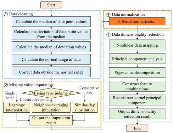
Figure 1.
Data preprocessing and dimensionality reduction process for high-current switchgear operation.
2.1. Data Cleaning
The primary objective of data cleaning is to eliminate measurement errors and abnormal disturbances, thereby improving data quality and establishing a reliable foundation for subsequent analysis. In this section, the MAD method is employed for data cleaning. MAD is a robust technique for detecting outliers by calculating the absolute deviations of all load values from the median load value. Due to its stability and broad applicability, MAD offers significant advantages in handling noisy datasets [26].
For the daily load data of a specific day, the data cleaning process proceeds as follows: First, the median of the 96 load values throughout the day are calculated. Second, the absolute deviation of each load point from the median is computed. Third, the median of all absolute deviations is obtained. Finally, based on actual requirements, a parameter is selected to define the acceptable range for the 96 daily load values. For load values falling outside the range, the cleaning process is given by
In the data cleaning phase, the parameter for the MAD method determines the threshold for outlier detection. Its value represents a trade-off between sensitivity and specificity. Based on preliminary data analysis and common practices in outlier detection [27], a value of was chosen to effectively filter out significant anomalies while preserving natural data fluctuations.
2.2. Missing Value Imputation
The missing value imputation ensures the completeness of the cleaned data and prevents analysis bias caused by data gaps. Different imputation methods are employed in this section to address various types of missing data scenarios [28].
(1) For cases where a single time point is missing within a day’s load data, Lagrange interpolation is employed for imputation. Typically, the two time steps before and after the missing point, totaling four data points, are used for interpolation fitting. According to numerical analysis theory, given points on a plane, of which are distinct, there exists a unique polynomial of degree at most that passes through points on the plane, which is expressed as
When determining this polynomial, the coordinates of the points are substituted into the equation, respectively, yielding
The Lagrange interpolation polynomial is given by
By substituting the coordinate corresponding to the missing value in the polynomial, the interpolated approximate value can be obtained.
(2) For cases where there are multiple consecutive missing data points within a single day, the missing load data for that time period are filled by averaging the corresponding load values from the same time periods of the previous and following days. This method is referred to as the same-day neighbor averaging imputation. Define the original high-current switchgear operation data sequence as , where represents recorded data and represents missing data. The relationship between and is given by
(3) For cases involving data missing over several consecutive days, the similar-day load substitution method is employed. Specifically, the missing data days are first classified as either weekdays or holidays. Then, the full-day load data from neighboring weekdays or holidays are selected to approximate and fill the missing values accordingly.
2.3. Data Normalization
After missing value imputation, data normalization is performed to scale data with different value ranges proportionally into a specific interval, thereby eliminating the influence of differing units among various indicators. The Z-Score standardization method, known for its wide applicability, transforms the original data into a dataset with a mean of zero and a variance of one [29]. It can be expressed as follows:
where represents the data after Z-Score normalization, is the original data before normalization, and and denote the mean and standard deviation of the original data, respectively.
2.4. Dimensionality Reduction
After data preprocessing, kernel principal component analysis (KPCA) is employed for dimensionality reduction [30]. KPCA can effectively handle high-dimensional operational data of high-current switchgear, improving data quality [31]. Suppose the dimensionality of the operational data is , with sampling points in each dimension. The preprocessed data is represented as . Through a nonlinear mapping, the data is projected into a high-dimensional feature space . At this stage, KPCA converts the problem into performing principal component analysis (PCA) on the matrix , which is expressed as follows:
Based on singular value decomposition or eigenvalue decomposition, the eigenvalues and eigenvectors of matrix are computed. Then, the eigenvectors are substituted into , which can be expressed as follows:
Considering that resides in a high-dimensional feature space, can be expressed as a linear combination of , which is formulated as follows:
where is the coefficient of transforming to . The mapping of in is represented as follows:
where is equal to , which corresponds to the inner product of and . Therefore, the reconstructed kernel principal components and their variance contribution rates are expressed as follows:
where represents the -th kernel principal component, and denotes the variance contribution rate of the -th kernel principal component. By setting a threshold for the cumulative variance contribution rate, different numbers of kernel principal components can be selected, thereby achieving dimensionality reduction.
3. Risk Assessment Method for High-Current Switchgear Based on Ensemble Learning
Machine learning can automatically predict and assess the operational risk level of high-current switchgear by analyzing historical operational data. Its adaptive learning capability allows the dynamic adjustment of the risk assessment model to accommodate changes in operating conditions, reducing reliance on human expertise. However, existing machine learning-based risk assessment methods have the following two limitations. On one hand, existing methods lack an accurate feature selection mechanism for switchgear operational data, leading to the inclusion of redundant features in the assessment model. This makes it difficult for the model to focus on the most influential features for risk evaluation, resulting in slow model convergence. On the other hand, the operating environment of switchgear is complex, and the risk assessment results are easily influenced by various nonlinear and disruptive factors. Existing methods lack effective risk assessment correction and optimization mechanisms, leading to low accuracy in the evaluation results.
On this basis, this paper proposes a risk assessment method for high-current switchgear based on ensemble learning. Compared to traditional learning methods, ensemble learning enhances the robustness and accuracy of risk assessment by leveraging the collaboration between multiple models, effectively overcoming the limitations of individual models in feature extraction, temporal modeling, and learning correction. The principle of the proposed method is shown in Figure 2. Specifically, in the first layer, the proposed algorithm uses an improved RF to perform feature extraction and selection on switchgear operational data. In the second layer, the proposed algorithm combines a gating optimization mechanism and an attention mechanism to construct a high-current switchgear risk assessment model based on an attention LSTM. The high-importance features selected in the first layer are used as input, capturing the key information of feature fluctuations and outputting the risk assessment results for the high current switchgear. In the third layer, the ABPNN model is embedded to correct and optimize the risk assessment results output from the second layer. Based on an adaptive genetic algorithm, the ABPNN parameters are dynamically adjusted to improve the accuracy and stability of the assessment.
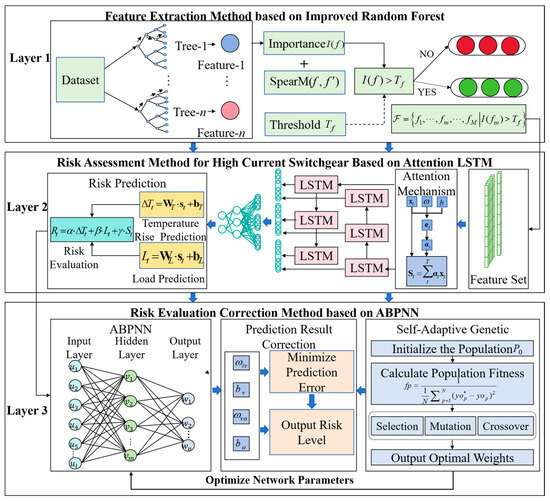
Figure 2.
Schematic of the risk assessment method for high-current switchgear based on ensemble learning.
3.1. Feature Extraction Method Based on Improved RF
As an embedded method, RF evaluates the importance of switchgear operational data features and performs feature selection by constructing multiple decision tree models. However, traditional RF overlooks the correlations among different features during the importance quantification process, resulting in a high redundancy among the extracted important features. This redundancy adversely affects the accuracy of subsequent temperature rise prediction and risk level assessment. Therefore, this section proposes an improved RF method that employs the Spearman correlation coefficient to measure the relationships between operational data features, enabling the identification and removal of highly correlated features to reduce redundancy.
The mean decrease in impurity (MDI) method is used to quantify feature importance [32]. Specifically, this method evaluates the contribution of each feature to the switchgear risk assessment by calculating the average decrease in impurity resulting from splits on that feature across all decision tree nodes. The Gini impurity, also known as Gini importance, is employed to measure feature importance. The Gini impurity at each decision tree node is calculated as follows:
where represents the number of feature categories, and represents the proportion of feature samples belonging to the category in node . Suppose node is split into left child node and right child node , their weighted average Gini impurity is calculated as follows:
where , , and represent the number of feature samples in the parent node, left child node, and right child node, respectively. Therefore, the decrease in impurity is calculated as follows:
where represents the Gini impurity of the parent node. The importance of feature can be obtained by calculating the sum of overall nodes where splits occur based on feature , which is expressed as follows:
where represents all nodes in the tree where splits occur based on feature , and represents the Spearman correlation coefficient between features and . A larger value of indicates a higher redundancy level of feature , which leads to a certain degree of reduction in its importance, where represents the set of all nodes in the tree where splits occur based on feature .
Set the importance threshold as , and retain all switchgear operational data features with importance greater than . The extracted feature set is denoted as .
In the feature extraction layer, the importance threshold for the improved RF method is crucial for selecting a concise yet informative feature set. This threshold was determined empirically by ranking features based on their importance scores and utilizing cross-validation to identify the subset of features that yields the best performance for the subsequent prediction task.
3.2. Risk Assessment Method for High-Current Switchgear Based on Attention LSTM
The feature values extracted by the random forest are input into the LSTM network for preliminary risk assessment. LSTM is adept at capturing long-term dependencies in time-series features, with a structure designed to adaptively remember or forget historical information, making it highly effective in intelligent risk assessment. However, traditional LSTM can encounter issues such as vanishing or exploding gradients when handling complex and diverse switchgear operational data, which can negatively affect the model’s training effectiveness and prediction accuracy. Therefore, this section optimizes the gating mechanism based on traditional LSTM and combines it with an attention mechanism, enabling the model to better focus on key information in the time series and improve its ability to capture short-term fluctuation features.
3.2.1. Optimizing the Gating Mechanism
Traditional LSTM consists of three components: the forget gate , the input gate , and the output gate . The forget gate is used to control the retention of historical switchgear operational states and information, the output gate controls the output of data, and the input gate manages the input of time-series data. The gating mechanism can be represented as follows:
where is the hidden state from the previous time period, is the input vector at the current time period, , , and are the weight matrices, , , and are the bias vectors, and is the sigmoid activation function.
Furthermore, optimize the gating mechanism. By adjusting the weight matrices and bias vectors, the error accumulation during backpropagation is effectively reduced, thereby mitigating gradient explosion and enhancing the model’s ability to handle complex time-series data. The optimized gating mechanism is represented as follows:
where is the cell state, is the weight matrix, is the bias vector, denotes element-wise multiplication, and is the hyperbolic tangent function.
3.2.2. Introducing the Attention Mechanism
In switchgear operation risk assessment, the impact of operational data at different time periods on the risk evaluation varies. For the LSTM network, effectively recognizing and distinguishing input features, giving higher attention to important features, and assigning higher weights typically enhance the model’s discriminative ability. Based on this, the attention mechanism is introduced to further optimize the LSTM. The attention mechanism calculates the corresponding probabilities of the input feature vectors and updates the weight matrices and biases at each iteration, gradually optimizing the weight combination of the input feature vectors to achieve the best prediction results. The calculation formula for the attention mechanism is as follows:
where represents the attention probability derived from the input vector at the -th time period, is the influence of the input feature vector at the -th time period on the output, i.e., the weight of the input vector , and is the output of the attention layer.
3.2.3. Switchgear Operation Risk Assessment
The operation risk assessment of switchgear involves multiple factors, including temperature rise, load, and equipment operating conditions. This section constructs a comprehensive switchgear operation risk assessment model based on attention LSTM. First, a temperature rise prediction model and a load prediction model are established. Based on these, a risk assessment model is constructed by incorporating equipment operating conditions to achieve accurate risk prediction for the switchgear. The temperature rise prediction model can be expressed as follows:
where is the temperature rise prediction value at the -th time period, is the weight matrix for temperature rise prediction, is the bias vector for temperature rise prediction, and is the weighted hidden state. Similarly, the load prediction model can be expressed as follows:
where is the load prediction value at the -th time period, is the weight matrix for load prediction, and is the bias vector for load prediction.
After obtaining the temperature rise and load prediction values, the risk assessment model is constructed by incorporating equipment operational status data. The model calculates the contribution of temperature rise, load, and equipment operating status to the operational risk, and the risk values of the switchgear at different time periods can be derived. The risk assessment model is expressed as follows:
where is the switchgear operational risk value at the -th time period, is the equipment operating status score, and , , and are the weight coefficients represent the contributions of temperature rise, load, and equipment operating status to the operational risk, respectively.
In the risk assessment model, the weight coefficients , and in Equation (29) represent the relative importance of temperature rise, load, and equipment status. In this study, these weights are assigned based on operational experience and historical fault statistics, reflecting the domain knowledge that temperature rise is a primary indicator of imminent risk. We acknowledge that a more objective determination of these weights is a valuable direction for future research. For instance, multi-physics simulation could be employed to establish a more rigorous quantitative relationship between these factors and the operational risk.
3.3. Risk Assessment Correction Method Based on ABPNN
Switchgear operational risk is influenced by the interaction of various factors, making it prone to deviations during risk assessment. BP neural networks, due to their strong generalization and self-organizing capabilities, can calibrate and optimize the assessment results. However, traditional BP neural networks are susceptible to the curse of dimensionality and the issue of training obtaining trapped in local optima, which leads to reduced calibration accuracy. Therefore, this section proposes the ABPNN, which introduces an adaptive genetic algorithm based on traditional neural networks. By dynamically adjusting network parameters, it improves training efficiency and prediction accuracy while effectively avoiding issues like local optima and overfitting, thus optimizing the performance of BP neural networks. Furthermore, the genetic algorithm adaptively adjusts the crossover and mutation probabilities to ensure population diversity and enhance the convergence of the model.
3.3.1. Network Architecture of ABPNN
The ABPNN switchgear operation risk assessment correction model adopts a three-layer network architecture, including an input layer, a hidden layer, and an output layer. The input layer consists of neurons , representing the influencing factors of operational risk. The hidden layer contains neurons , which is responsible for processing the input data and generating intermediate results that are passed to the subsequent layers. The output layer consists of neurons , and the output values represent the specific operational risk levels. The input and output of the -th neuron in the ABPNN hidden layer are represented as follows:
where represents the connection weight from the input layer to the hidden layer.
The input and output of the -th neuron in the output layer are represented as follows:
where represents the connection weights from the hidden layer to the output layer. is the activation function between the hidden layer and the output layer, typically chosen as the sigmoid function. The weights and can be adjusted by calculating the error of the output values.
The input layer of the ABPNN switchgear operation risk assessment correction model consists of 10 neurons, i.e., operational lifespan (), historical fault condition (), load current (), busbar temperature (), contact temperature (), ambient temperature (), ambient humidity (), conductor contact resistance (), contact area (), and fan status (). The output layer of the model outputs the corrected switchgear operational risk levels. Therefore, the number of neurons in the output layer is set to 3, i.e., , , and , with each neuron outputting values of 0 or 1. The output values of , , and and their corresponding switchgear risk levels are shown in Table 2.
Table 2.
Correspondence between output layer neuron values and switchgear risk levels.
3.3.2. Risk Assessment Correction Method Based on ABPNN
During risk assessment correction, the influencing factors and risk levels of switchgear operational risk are first determined, and the input data is mapped to the range to obtain the input layer neurons and output layer data for the ABPNN. For real-valued influencing factors, such as operational lifespan (), load current (), busbar temperature (), contact temperature (), ambient temperature (), ambient humidity (), conductor contact resistance (), and contact area (), normalization has already been performed during data preprocessing, allowing them to be directly input into the ABPNN. For categorical influencing factors, such as historical fault condition () and fan status (), the independent variable assignment method shown in Table 3 can be used.
Table 3.
Assignment of impact factors for switchgear temperature rise.
Then, the alternative network structure is selected, which involves determining the number of neurons in the hidden layer. Several integers within the range are chosen as the number of neurons in the hidden layer. The network is trained using a small sample dataset, and the corresponding convergence errors are recorded. The number of hidden layer neurons with the smallest convergence error during training is selected as the optimal network structure. After determining the network structure, the ABPNN parameters are initialized, including the connection weights from the input layer to the hidden layer, the weights from the hidden layer to the output layer, the threshold for the hidden layer, and the threshold for the output layer. In addition, set the initial learning rate for model training and the desired minimum training error threshold. Finally, the ABPNN takes the influence factor data representing the switchgear status output by the LSTM network as input and outputs the predicted risk level encoding. Through supervised learning, the network weights and thresholds are continuously adjusted using the backpropagation algorithm to minimize the error between the predicted output and the true risk level. By deeply integrating and reassessing the predicted values from the LSTM network and the switchgear status features, the prediction bias is corrected, ultimately outputting the optimized operational risk level assessment.
3.3.3. Adaptive Genetic Algorithm for Optimizing Network Parameters
To improve the training efficiency and prediction accuracy of the ABPNN model, avoid issues such as local optima and overfitting during training, and further enhance the correction performance, this paper introduces an adaptive genetic algorithm to optimize the core parameters of ABPNN. The steps are as follows.
Step 1: The initial network parameters of ABPNN are encoded to generate multiple distinct individuals, and the population size is set as . As the initial population , these individuals are then input into the genetic algorithm.
Step 2: The fitness of the population is used to measure an individual’s ability to survive in the environment. A higher fitness value indicates a better individual’s genes, which corresponds to a greater likelihood of survival and reproduction. In this model, each individual’s output is calculated using sample data and the initialized ABPNN model, and the result is compared with the desired output. The error value is calculated to evaluate the quality of the individual’s genes, which determines their fitness. The individual’s fitness value is calculated as follows:
where represents the number of training samples, is the predicted output value of the sample, and is the actual output value of the sample. By repeating the process, the fitness values of all individuals in the -th generation of the population can be derived.
Step 3: Initialize the maximum number of iterations for the genetic algorithm, the crossover probability within the range , and the mutation probability within the range .
Step 4: Use the roulette wheel selection method to perform optimal selection of individuals from the population. Based on the fitness values of the individuals in the population, the probability of each individual being inherited and the cumulative probability are calculated as follows:
A random number between is generated. If the cumulative probability of an individual is greater than , then this individual is selected to stay; otherwise, another individual is chosen such that . Step 4 is repeated until every individual in the population has been selected once.
Step 5: Based on the changes in the fitness values of the population individuals, the crossover and mutation probabilities are dynamically adjusted to form a new population. Set the initial values and the initial crossover probability and the initial mutation probability are given by
where , , , and are fixed values.
The new population is then obtained, and its fitness values are calculated. If the fitness values are widely dispersed, the probabilities can be reduced to retain the better-performing individuals in the population. If an individual’s fitness value indicates that it has become trapped in a local optimum, the probabilities of escaping the local optimum are increased, ensuring individual diversity.
Step 6: Repeat steps 4 to 6 until the maximum number of iterations is reached. Output and decode the optimal individual, and analyze to obtain the optimal parameters for the ABPNN. Update the ABPNN based on the optimal parameters.
The algorithm is summarized in Table 4.
Table 4.
Algorithm table for the risk assessment method for high-current switchgear based on ensemble learning.
4. Simulation Analysis
To systematically verify the effectiveness and superiority of the method for operation risk assessment of high-current switchgear based on ensemble learning, a case study verification under actual operating conditions is conducted. The software used for simulation analysis is MATLAB R2024a (24.1.0.2537033), 64-bit (win64), released on 21 February 2024. Simulation parameters are shown in Table 5. The experimental data are derived from the actual operation record dataset of multiple high-current switchgears in a regional distribution network, which mainly includes 960 sets of equipment monitoring data for high-current switchgears and historical load current data recorded by the SCADA system. The equipment monitoring data cover the name of the monitoring device, specific location information, sampling time, load current, and the temperatures of the upper and lower contacts at the A/B/C three-phase moving contacts. The SCADA system records basic information such as load current and contact temperature, as well as multi-dimensional information including knife switch temperature, ambient temperature, and cabinet fan status. All data are preprocessed in accordance with the method described in Section 2. Data cleaning is performed using the MAD method, missing values are handled by Lagrange interpolation and similar-day imputation, dimensional differences are eliminated through Z-Score standardization, and KPCA technology is applied for dimensionality reduction in high-dimensional features to retain key information while improving model training efficiency. A total of 720 preprocessed datasets are selected for training and learning, and 240 of them are finally chosen for testing.
Table 5.
Simulation parameters [33,34,35].
To systematically verify the effectiveness and superiority of the method for operation risk assessment of high-current switchgear based on ensemble learning, a case study verification under actual operating conditions is conducted. The overall simulation process is illustrated in Figure 3.
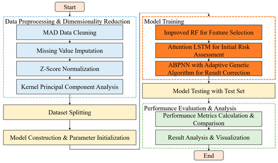
Figure 3.
Flowchart of the overall simulation process.
To comprehensively evaluate the performance of the proposed algorithm, three representative methods were selected as baselines. Baseline 1 [36]: It adopts an improved RF model for feature selection and preliminary evaluation, and uses the traditional LSTM to predict the load evolution trend and temperature rise process. However, it has limitations in predicting dynamic change trends. Baseline 2 [37]: It employs an improved LSTM network with an attention mechanism for evaluation. Baseline 2 can effectively capture the temporal features in the data, but lacks an effective correction mechanism for systematic prediction biases that may be caused by complex nonlinear disturbance factors. Baseline 3 [38]: It utilizes the traditional LSTM and ABPNN for risk assessment. Based on its nonlinear fitting ability, a direct mapping model from multi-dimensional operating parameters to risk levels is established. Nevertheless, it is difficult to capture the long-term dependencies of load fluctuations and temperature rise evolution, and thus cannot effectively identify key temporal features.
Taking temperature rise prediction as an example, the algorithm’s performance is verified. The following performance metrics are considered: the coefficient of determination (R2), mean absolute error (MAE), mean absolute percent error (MAPE), and root mean square error (RMSE). The formulas are as follows:
R2:
MAE:
MAPE:
RMSE:
where is the total number of samples, represents the predicted value of the -th sample, and represents the true value of the -th sample. and focus on describing the reliability of the model, while and focus on describing the prediction accuracy of the model.
Figure 4 presents a comparison of temperature rise prediction results for 30 samples by various algorithms when the load current is 1 kA. Figure 5 shows the corresponding comparison of relative errors in the prediction results. Table 5 displays the results of various indicators for algorithms. The data in Figure 4 and Figure 5, and Table 6 indicate that R2 of the proposed algorithm reaches 0.981, which is 15.4%, 4.9%, and 24.8% higher than that of Baseline 1, Baseline 2, and Baseline 3, respectively, demonstrating a significant enhancement in fitting ability. Compared with Baseline 1, Baseline 2, and Baseline 3, MAE of the proposed algorithm is reduced by 64.7%, 48.7%, and 72.8%, respectively; MAPE is reduced by 65.1%, 49.5%, and 73.5%, respectively; and RMSE is reduced by 63.9%, 45.3%, and 69.8%, respectively, showing lower prediction errors and higher accuracy. The reason is that, in contrast to Baseline 1, Baseline 2, and Baseline 3, the proposed algorithm makes full use of a multi-level integrated learning framework. It introduces an attention mechanism based on the LSTM in the first layer, effectively capturing long-term dependent features in time series and achieving accurate prediction of load evolution trends and temperature rise processes. Meanwhile, the second layer adopts an improved RF for feature extraction, and by optimizing the feature selection mechanism and tree structure parameters, it improves the model’s ability to screen key operational features and the accuracy of preliminary evaluation. In addition, the third layer further constructs a prediction correction model based on ABPNN, which can effectively correct the risk assessment results output by LSTM.

Figure 4.
Comparison of temperature rise prediction results of various algorithms under fixed current.
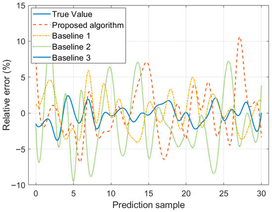
Figure 5.
Comparison of relative errors in temperature rise prediction results.
Table 6.
Results of various indicators for algorithms.
Figure 6 shows the prediction results of switchgear contact temperature rise under different load currents for various algorithms. The proposed algorithm’s prediction curve closely matches the real temperature rise curve within the interval. Its principle is similar to that in Figure 4, where the first layer of the ensemble learning framework extracts key features through an improved RF. The second layer then uses an attention LSTM to accurately capture the temporal dependencies in the temperature rise process. The third layer uses the ABPNN model for final correction of the prediction results. Its nonlinear fitting ability corrects the residual bias from the previous models. This allows for the accurate restoration of the complex physical relationship between temperature rise and load current. The model demonstrates high accuracy in temperature rise prediction under complex operating conditions.
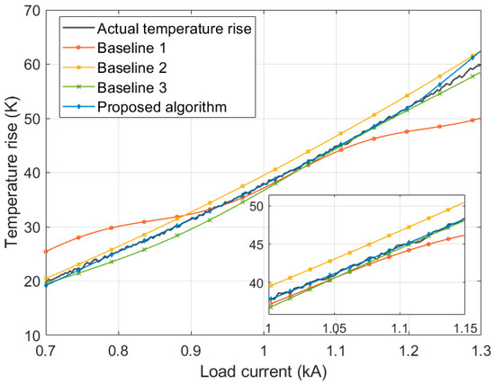
Figure 6.
Prediction of switchgear contact temperature rise under different load currents.
Figure 7 shows the RMSE convergence curves of different algorithms during the training process. Compared to the convergence values of Baseline 1, Baseline 2, and Baseline 3, RMSE of the proposed algorithm is reduced by 64.25%, 45.34%, and 69.83%, and the convergence speed is improved by 44.90%, 22.86%, and 6.90%, respectively. This is due to the use of an improved RF model for feature extraction and selection. By combining information gain ratio and feature stability for joint selection, and introducing the Spearman correlation coefficient to identify and remove highly correlated redundant features, it ensures that the feature set input into the subsequent deep learning models consists of highly correlated key influencing factors. This makes the learning process more efficient and significantly accelerates the convergence speed. In the second layer of the ensemble learning framework, an improved LSTM network with an attention mechanism is constructed. The switchgear operational data exhibits complex temporal dependencies, and the contribution of features at different time periods to risk assessment varies. The introduced temporal attention module enables the LSTM to dynamically assign weights to input features at different time steps, focusing on the most decisive information for the current prediction. This greatly enhances the model’s ability to capture complex temporal features in the data, making it particularly sensitive to anomalous data. At the same time, the optimized gating mechanism effectively alleviates the gradient issues in long sequences, ensuring stable training of the model in deep networks. The introduction of the attention mechanism allows the model to more effectively identify and utilize key information, preventing overfitting to less important information. This enables the model to find the global optimal solution more quickly during training and achieve lower prediction errors.
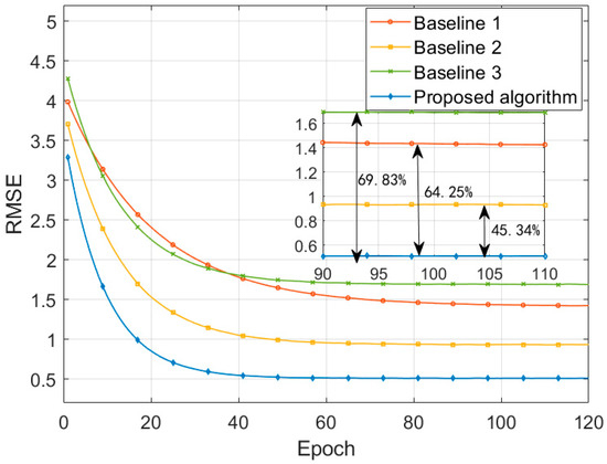
Figure 7.
RMSE convergence curves for different algorithms.
Table 7 shows the prediction accuracy of different algorithms for samples at various risk levels. The proposed algorithm demonstrates a significant accuracy advantage, particularly in identifying high-risk (Level V) cases. Based on historical fault data, switchgear temperature, and potential safety hazards, the switchgear risk level can be classified into five levels, as shown in Table 8. Compared to Baseline 1, Baseline 2, and Baseline 3, the overall prediction accuracy has increased by 22.7%, 11.3%, and 5.1%, respectively. The high-risk recognition accuracy has increased by 29.63%, 12.90%, and 9.37%, respectively. The fundamental reason lies in the collaborative effect of the models at each layer in the ensemble learning framework. The attention mechanism-based LSTM is able to dynamically focus on and weight the key information in the input temporal data. For high-risk features, the attention mechanism assigns higher weights to these features, allowing for early-stage accurate warning and classification of potential Level V fault risks. When the second layer provides a preliminary risk level, especially when it is close to Level V, ABPNN, through its nonlinear mapping ability and adaptive learning mechanism, performs secondary classification and optimization for these boundary or ambiguous samples. This minimizes potential misclassification at the final classification output layer, ensuring the model has higher confidence and reliability, significantly reducing the probability of underestimating high-risk events.
Table 7.
Results of various indicators for algorithms.
Table 8.
Risk level table.
The confusion matrix shown in Figure 8 demonstrates the classification performance of the proposed algorithm on risk samples. The results show that the proposed algorithm achieves recognition accuracy of 94.2%, 94.8%, 94.0%, 93.2%, and 97.2% for risk levels I, II, III, IV, and V, respectively, maintaining high recognition accuracy across all levels. The reason is that, in the ensemble learning framework, ABPNN serves as the final correction layer, performing deep fusion and optimization of the preliminary risk assessment results from the first two layers. Traditional BP neural networks are prone to becoming stuck in local optima or suffering from the curse of dimensionality, but the adaptive genetic algorithm introduced in this paper effectively overcomes these shortcomings. It dynamically optimizes the network structure and weights of ABPNN, enhancing its global search capability, and enhances the learning effect of nonlinear features by adaptively adjusting the learning rate and error feedback mechanism. Even if the first two layers exhibit slight deviations under certain complex conditions, ABPNN can precisely correct these deviations through its adaptive correction ability, significantly improving the accuracy of the final risk level classification and the robustness of the system.
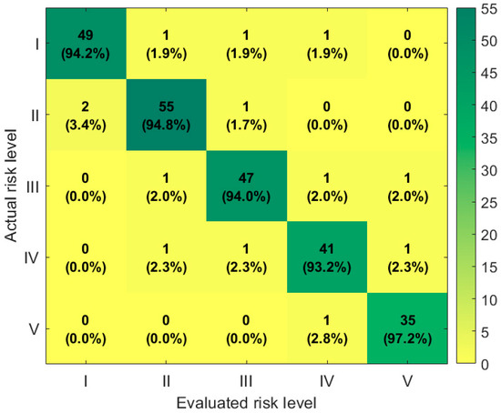
Figure 8.
Confusion matrix for risk level classification of the proposed method.
5. Conclusions
To address the problem of accurately assessing the operational risks of switchgears under complex operating environments and severe load fluctuations, this paper has proposed a method for operation risk assessment of high-current switchgears based on ensemble learning. First, we have preprocessed and reduced the dimensionality of multi-source operational data to improve data quality. Then, via a multi-layer integrated learning framework, we have used improved RF to extract key features in the first layer, combined an attention mechanism with LSTM to capture temporal features and assess risks in the second layer, and corrected results with ABPNN fused with an adaptive genetic algorithm to enhance assessment performance in the third layer. Simulation results show that in temperature rise prediction, the proposed algorithm significantly improves the goodness-of-fit indicator R2, with increases of 15.4%, 4.9%, and 24.8% compared to Baseline 1, Baseline 2, and Baseline 3, respectively. Particularly, the accuracy of high-risk level identification is more prominently improved, with increases of 29.63%, 12.90%, and 9.37%, respectively. These results fully demonstrate that the proposed multi-layer integrated learning framework, through the collaborative operation of each process, effectively enhances the accuracy of temperature rise prediction and the reliability of operation risk assessment for high-current switchgears. Moreover, it exhibits excellent performance in identifying high-risk levels under complex operating conditions, providing strong support for the safe operation of switchgears.
Future research will optimize the algorithm structure through lightweight technologies such as model compression and knowledge distillation to significantly improve real-time processing capabilities. Meanwhile, by combining transfer learning methods to transfer knowledge from pre-trained models to new domains, the generalization performance of the algorithm in different application scenarios will be enhanced. In subsequent work, further exploration will be conducted on the setting of key model parameters, and targeted simulations will be carried out to obtain the basis for parameter optimization, thereby improving the adaptability and reliability of the risk assessment model to the complex operating conditions of high-current switchgear.
Author Contributions
Conceptualization, W.X., P.C., C.Y. and B.L.; methodology, W.X., P.C., C.Y. and Z.W.; software, W.X., P.C., C.Y. and Y.H.; validation, Z.W., S.L. and Y.H.; formal analysis, W.X., P.C., C.Y. and J.Z.; investigation, W.X., P.C., S.L., Y.H. and J.Z.; resources, W.X.; data curation, P.C., C.Y. and Z.W.; writing—original draft preparation, W.X., P.C., C.Y., Z.W., S.L., Y.H. and J.Z.; writing—review and editing, W.X., P.C. and B.L.; funding acquisition, W.X. All authors have read and agreed to the published version of the manuscript.
Funding
This work was supported by the Science and Technology Program of China Southern Power Grid Corporation under grant number 031900KC24090042.
Data Availability Statement
The data that support the findings of this study are available from the corresponding author, Weidong Xu, upon reasonable request.
Conflicts of Interest
Authors Weidong Xu, Peng Chen, Cong Yuan, and Zhi Wang were employed by Dongguan Power Supply Bureau Guangdong Power Grid Company. The remaining authors declare that the research was conducted in the absence of any commercial or financial relationships that could be construed as a potential conflict of interest. The company had no role in the design of the study, in the collection, analyses, or interpretation of data; in the writing of the manuscript, or in the decision to publish the results.
References
- Wang, L.; Li, X.; Lin, J.; Jia, S. Studies of Modeling and Simulation Method of Temperature Rise in Medium-Voltage Switchgear and Its Optimum Design. IEEE Trans. Compon. Packag. Manuf. Technol. 2018, 8, 439–446. [Google Scholar] [CrossRef]
- Li, J.; Sun, Y.; Dong, N.; Zhao, Z. A Novel Contact Temperature Calculation Algorithm in Distribution Switchgears for Condition Assessment. IEEE Trans. Compon. Packag. Manuf. Technol. 2019, 9, 279–287. [Google Scholar] [CrossRef]
- Muhamad, N.A.; Visa Musa, I.; Abdul Malek, Z.; Salah Mahdi, A. Classification of Partial Discharge Fault Sources on SF6 Insulated Switchgear Based on Twelve By-Product Gases Random Forest Pattern Recognition. IEEE Access 2020, 8, 212659–212674. [Google Scholar] [CrossRef]
- Yanabu, S.; Nishiwaki, S.; Mizoguchi, H.; Shimokawara, N.; Murayama, Y. High Current Interruption by SF6 Disconnecting Switches in Gas Insulated Switchgear. IEEE Trans. Power Appar. Syst. 1982, PAS-101, 1105–1114. [Google Scholar] [CrossRef]
- Wang, Y.; Yan, J.; Yang, Z.; Zhang, W.; Wang, J.; Geng, Y.; Srinivasan, D. A Class Alignment Multisource Domain Adaptation for Partial Discharge Condition Assessment With Unknown Faults in GIS. IEEE Internet Things J. 2025, 12, 19955–19971. [Google Scholar] [CrossRef]
- Xuan, Y.; Si, W.; Zhu, J.; Sun, Z.; Zhao, J.; Xu, M.; Xu, S. Multi-Model Fusion Short-Term Load Forecasting Based on Random Forest Feature Selection and Hybrid Neural Network. IEEE Access 2021, 9, 69002–69009. [Google Scholar] [CrossRef]
- Sotnikov, D.; Lyly, M. and Salmi, T. Prediction of 2G HTS Tape Quench Behavior by Random Forest Model Trained on 2-D FEM Simulations. IEEE Trans. Appl. Supercond. 2023, 33, 6602005. [Google Scholar] [CrossRef]
- Shaikh, M.A.H.; Barbé, K. Study of Random Forest to Identify Wiener–Hammerstein System. IEEE Trans. Instrum. Meas. 2021, 70, 6500712. [Google Scholar] [CrossRef]
- Wassan, J.T.; Wang, H.; Zheng, H. Developing a New Phylogeny-Driven Random Forest Model for Functional Metagenomics. IEEE Trans. NanoBiosci. 2023, 22, 763–770. [Google Scholar] [CrossRef]
- Yu, M.; Xu, F.; Hu, W.; Sun, J.; Cervone, G. Using Long Short-Term Memory (LSTM) and Internet of Things (IoT) for Localized Surface Temperature Forecasting in an Urban Environment. IEEE Access 2021, 9, 137406–137418. [Google Scholar] [CrossRef]
- Wang, H.; Lu, B.; Li, J.; Liu, T.; Xing, Y.; Lv, C.; Cao, D.; Li, J.; Zhang, J.; Hashemi, E. Risk Assessment and Mitigation in Local Path Planning for Autonomous Vehicles With LSTM Based Predictive Model. IEEE Trans. Autom. Sci. Eng. 2022, 19, 2738–2749. [Google Scholar] [CrossRef]
- Tan, X.; Li, Z.; Wang, X.; Liu, K.; Zhang, C.; Wu, G. Research on Vehicle Rollover Risk Prediction Based on CNN-LSTM and Unscented Kalman Filter Algorithm. IEEE Trans. Instrum. Meas. 2025, 74, 6503312. [Google Scholar] [CrossRef]
- Panda, R.; Tiwari, P.K. Cross-Entropy Based Risk Assessment and Forecasting of Secured Hybrid System Using Bi-LSTM Based AM Deep Learning Model. IEEE Trans. Ind. Appl. 2025, 61, 4661–4674. [Google Scholar] [CrossRef]
- Chen, G.; Li, L.; Zhang, Z.; Li, S. Short-Term Wind Speed Forecasting With Principle-Subordinate Predictor Based on Conv-LSTM and Improved BPNN. IEEE Access 2020, 8, 67955–67973. [Google Scholar] [CrossRef]
- Dai, P.; Bao, J.; Gong, Z.; Gao, M.; Xu, Q. Lifetime Prediction of IGBT by BPNN Based on Improved Dung Beetle Optimization Algorithm. IEEE Trans. Device Mater. Reliab. 2025, 25, 341–351. [Google Scholar] [CrossRef]
- Gu, F.-C. Identification of Partial Discharge Defects in Gas-Insulated Switchgears by Using a Deep Learning Method. IEEE Access 2020, 8, 163894–163902. [Google Scholar] [CrossRef]
- Li, L.; Tang, J.; Liu, Y. Partial Discharge Recognition in Gas Insulated Switchgear Based on Multi-Information Fusion. IEEE Trans. Dielectr. Electr. Insul. 2015, 22, 1080–1087. [Google Scholar] [CrossRef]
- Alsumaidaee, Y.A.M.; Paw, J.K.S.; Yaw, C.T.; Tiong, S.K.; Chen, C.P.; Yusaf, T.; Benedict, F.; Kadirgama, K.; Hong, T.C.; Abdalla, A.N. Fault Detection for Medium Voltage Switchgear Using a Deep Learning Hybrid 1D-CNN-LSTM Model. IEEE Access 2023, 11, 97574–97589. [Google Scholar] [CrossRef]
- Miao, Y.; Zhang, Y.; Chen, F.; Wang, Z. Analog Circuit Incipient Fault Detection Based on Attention Mechanism and Fully Convolutional Network. IEEE Access 2024, 12, 137247–137258. [Google Scholar] [CrossRef]
- Wang, Y.; Yan, J.; Zhang, W.; Yang, Z.; Wang, J.; Geng, Y.; Srinivasan, D. Mutitask Learning Network for Partial Discharge Condition Assessment in Gas-Insulated Switchgear. IEEE Trans. Ind. Inform. 2024, 20, 11998–12009. [Google Scholar] [CrossRef]
- Wang, Y.; Yan, J.; Qi, M.; Yang, Z.; Wang, J.; Geng, Y. Collaborative Domain Adaptation Network for Partial Discharge Source Localization in Gas-Insulated Switchgear. IEEE Trans. Instrum. Meas. 2023, 72, 3512312. [Google Scholar] [CrossRef]
- Hussain, G.A.; Hassan, W.; Mahmood, F.; Kay, J.A. Partial Discharge Based Risk Assessment Framework for MV Switchgear Containing Electrical Defects. IEEE Trans. Ind. Appl. 2023, 59, 7868–7875. [Google Scholar] [CrossRef]
- Kim, E.-H.; Oh, S.-K.; Pedrycz, W. Design of Reinforced Interval Type-2 Fuzzy C-Means-Based Fuzzy Classifier. IEEE Trans. Fuzzy Syst. 2018, 26, 3054–3068. [Google Scholar] [CrossRef]
- Tuyet-Doan, V.N.; Youn, Y.W.; Choi, H.S.; Kim, Y.H. Shared Knowledge-Based Contrastive Federated Learning for Partial Discharge Diagnosis in Gas-Insulated Switchgear. IEEE Access 2024, 12, 34993–35007. [Google Scholar] [CrossRef]
- Zhou, N.; Xu, Y. A Prioritization Method for Switchgear Maintenance Based on Equipment Failure Mode Analysis and Integrated Risk Assessment. IEEE Trans. Power Deliv. 2024, 39, 728–739. [Google Scholar] [CrossRef]
- Guha, S.; Khan, F.A.; Stoyanovich, J.; Schelter, S. Automated Data Cleaning Can Hurt Fairness in Machine Learning-Based Decision Making. IEEE Trans. Knowl. Data Eng. 2024, 36, 7368–7379. [Google Scholar] [CrossRef]
- Romo-Chavero, M.A.; Alatorre, G.D.L.R.; Cantoral-Ceballos, J.A.; Pérez-Díaz, J.A.; Martinez-Cagnazzo, C. A Hybrid Model for BGP Anomaly Detection Using Median Absolute Deviation and Machine Learning. IEEE Open J. Commun. Soc. 2025, 6, 2102–2116. [Google Scholar] [CrossRef]
- Malambo, L.; Heatwole, C.D. A Multitemporal Profile-Based Interpolation Method for Gap Filling Nonstationary Data. IEEE Trans. Geosci. Remote Sens. 2016, 54, 252–261. [Google Scholar] [CrossRef]
- Passalis, N.; Tefas, A.; Kanniainen, J.; Gabbouj, M.; Iosifidis, A. Deep Adaptive Input Normalization for Time Series Forecasting. IEEE Trans. Neural Netw. Learn. Syst. 2020, 31, 3760–3765. [Google Scholar] [CrossRef]
- Mo, D.; Huang, S.H. Fractal-Based Intrinsic Dimension Estimation and Its Application in Dimensionality Reduction. IEEE Trans. Knowl. Data Eng. 2012, 24, 59–71. [Google Scholar]
- Alghamdi, T.A.; Javaid, N. A Survey Of Preprocessing Methods Used For Analysis Of Big Data Originated From Smart Grids. IEEE Access 2022, 10, 29149–29171. [Google Scholar] [CrossRef]
- Ghubaish, A.; Yang, Z.; Erbad, A.; Jain, R. LEMDA: A Novel Feature Engineering Method for Intrusion Detection in IoT Systems. IEEE Internet Things J. 2024, 11, 13247–13256. [Google Scholar] [CrossRef]
- Zhou, M.; Zhang, H.; Zhang, W.; Yi, Y. An Improved Random Forest Algorithm-Based Fatigue Recognition With Multiphysical Feature. IEEE Sens. J. 2023, 23, 26195–26201. [Google Scholar] [CrossRef]
- Zhu, J.; Chen, F.; Liu, S.; An, Y.; Wu, N.; Zhao, X. Multi-Objective Planning Optimization of Electric Vehicle Charging Stations With Coordinated Spatiotemporal Charging Demand. IEEE Trans. Intell. Transp. Syst. 2025, 26, 1754–1768. [Google Scholar] [CrossRef]
- Parizad, A.; Hatziadoniu, C. Deep Learning Algorithms and Parallel Distributed Computing Techniques for High-Resolution Load Forecasting Applying Hyperparameter Optimization. IEEE Syst. J. 2022, 16, 3758–3769. [Google Scholar] [CrossRef]
- Neto, M.P.; Paulovich, F.V. Explainable Matrix—Visualization for Global and Local Interpretability of Random Forest Classification Ensembles. IEEE Trans. Vis. Comput. Graph. 2021, 27, 1427–1437. [Google Scholar] [CrossRef]
- Qin, H.; Xiong, Z.; Li, Y.; El-Yacoubi, M.A.; Wang, J. Attention BLSTM-Based Temporal-Spatial Vein Transformer for Multi-View Finger-Vein Recognition. IEEE Trans. Inf. Forensics Secur. 2024, 19, 9330–9343. [Google Scholar] [CrossRef]
- Bai, L.; An, Y.; Sun, Y. Measurement of Project Portfolio Benefits With a GA-BP Neural Network Group. IEEE Trans. Eng. Manag. 2024, 71, 4737–4749. [Google Scholar] [CrossRef]


Disclaimer/Publisher’s Note: The statements, opinions and data contained in all publications are solely those of the individual author(s) and contributor(s) and not of MDPI and/or the editor(s). MDPI and/or the editor(s) disclaim responsibility for any injury to people or property resulting from any ideas, methods, instructions or products referred to in the content. |
© 2025 by the authors. Licensee MDPI, Basel, Switzerland. This article is an open access article distributed under the terms and conditions of the Creative Commons Attribution (CC BY) license (https://creativecommons.org/licenses/by/4.0/).