Abstract
Top-bottom combined blowing converter steelmaking involves complex thermodynamic and kinetic processes, and predictive modeling has long been a key focus in steelmaking research. This paper proposes a kinetic process prediction model with on-site applicability. Based on actual production data, machine learning models (BP neural network, random forest, XGBoost) are employed to predict Tapping Steel Oxygen (TSO) content, which is then used as input for the kinetic model. An optimized theoretical decarburization kinetic model is selected and validated against measured Tapping Steel Carbon (TSC) data. The key innovation lies in the integration of converter control parameters into the kinetic model through a data-driven cyclic iteration algorithm. Comparison of prediction accuracy before and after integration shows that the model’s TSC prediction within the range [−0.2, +0.2] improves by 6.26%. This work presents a novel approach for enhancing kinetic models via control parameter integration, offering effective guidance for real-time monitoring and optimization in converter steelmaking.
1. Introduction
During the blowing process of basic oxygen furnace (BOF) steelmaking, it is difficult to obtain accurate and continuous dynamic measurements of key process variables such as temperature and composition changes [1]. As one of the most critical stages in steel production, the core and most challenging aspect of BOF operation lies in the dynamic control of the blowing process [2]. Due to the lack of effective in-process monitoring methods, the current operation often involves a certain degree of blindness and subjectivity, which may lead to excessive top-blowing oxygen supply [3], resulting in unnecessary consumption of hot metal and other raw materials [4], and consequently increasing energy consumption and production costs. By integrating kinetic theoretical models with actual process control parameters through correction mechanisms, a comprehensive kinetic model for the BOF process can be established. This approach enables a more accurate representation of the internal evolution during steelmaking, forming the theoretical foundation for soft sensing in the smelting process [5].
To address the prediction challenges in BOF steelmaking, extensive research has been conducted by scholars worldwide. Lin Dong et al. [6] developed a mechanistic model based on the analysis of combined blowing mechanisms and dynamic mass and heat balances during the blowing process, which reflects the variations in steel and slag compositions. Ma Dewen et al. [7] established a BOF prediction model based on the reaction kinetics in the jet impact zone, emulsion zone, and slag-metal interface, aiming to predict the end-point compositions of steel and slag. Dogan N et al. [8] proposed a comprehensive kinetic model for decarburization in oxygen steelmaking based on reaction kinetics. Ik Y et al. [9] developed a process simulation model consisting of a reaction submodel and a scrap melting/dissolution submodel, successfully explaining the redox behaviors of phosphorus and manganese during BOF steelmaking. Although these studies have established relatively mature kinetic and mechanistic models, many model parameters either lack theoretical calculation methods or are inherently unmeasurable, making it difficult to apply them directly in industrial practice.
In this study, selected process control parameters influencing the decarburization reaction are incorporated into the kinetic model, along with optimizable correction parameters. These correction parameters are then optimized using actual production data to enhance model accuracy and facilitate direct operational adjustments in practical BOF operations. The research methodology is as follows: First, existing kinetic models for the decarburization reaction are reviewed and evaluated for their applicability and predictive accuracy in real-world production. A suitable kinetic model capable of integrating control parameters for practical guidance is selected. Using actual plant data, the hit rates for TSC (Tapping Secondary Carbon) and TSO (Tapping Sample Oxygen) predictions are calculated to assess the baseline performance of the original kinetic model. Subsequently, key BOF control parameters are integrated into the kinetic model, and the prediction accuracy is compared before and after the integration to evaluate the improvement. Finally, three machine learning models—Back Propagation (BP) neural network, Random Forest, and XGBoost—are developed to predict the end-point TSO carbon content. These predicted values are used as inputs to the kinetic model, thereby closing the modeling loop and enabling real-time characterization of carbon evolution within the furnace.
2. Prediction of End-Point TSO Carbon Content Using Machine Learning Models
Predicting the end-point carbon content in basic oxygen furnace (BOF) steelmaking is a crucial foundation for achieving stable control of molten steel composition [10]. The Back Propagation (BP) neural network is a multi-layer feedforward neural network based on the error back-propagation algorithm, which exhibits strong nonlinear fitting capability and is therefore suitable for modeling complex, mechanism-unclear processes with intricate variable interactions [11]. The Random Forest model is an ensemble learning method composed of multiple decision trees; it improves prediction stability through voting or averaging strategies and is particularly effective for problems with high-dimensional features, moderate sample sizes, and requirements for model interpretability [12]. The Bayesian optimization using random forest (forest_minimize) converges stably within 15–20 iterations, with the objective function (e.g., carbon deviation) showing consistent improvement and saturation. Repeated trials confirm low variation in optimal solutions, demonstrating good robustness due to the ensemble nature of the random forest surrogate model. XGBoost (Extreme Gradient Boosting) is an optimized algorithm built on the gradient boosting framework, which supports regularization to prevent overfitting and enables parallel computation for enhanced efficiency [13]. In this work, these three data-driven modeling approaches were employed to predict the end-point steel composition in BOF operations, yielding predicted values of the tapping steel oxygen (TSO) carbon content. Subsequently, the predicted TSO results were used as input conditions for a kinetic process prediction model, enabling further optimization and closing the loop of the dynamic process simulation. Figure 1 shows the flowchart of the research methodology adopted in this study.
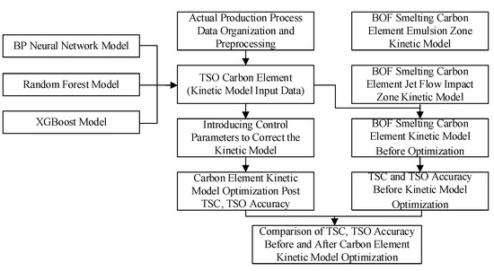
Figure 1.
Flowchart of the research methodology adopted in this study.
2.1. Preprocessing and Feature Selection
The raw data used in this study were collected from actual production records of the entire basic oxygen furnace (BOF) steelmaking process at a steel plant. Input parameters were subjected to data preprocessing to ensure a relatively stable and consistent operational condition. Table 1 presents the statistical summary of the data cleaning process.

Table 1.
Statistics of cleaned parameter data.
The cleaned process parameters were further constrained within defined screening ranges, as listed in Table 2. Each heat sample is represented by 11 input features: oxygen supply time, total blowing time, oxygen consumption for carbon reduction, hot metal temperature at charging, actual hot metal weight, actual scrap weight, lime addition, lightly burned dolomite addition, pellet addition, dynamic pellet addition, and hot metal carbon content. The output variable is the end-point carbon content of the molten steel at the end of the blow. These screening ranges were determined based on long-term operational data, equipment limitations, and metallurgical constraints observed at the production site, ensuring that the cleaned dataset reflects realistic and industrially feasible operating conditions.
Table 2.
Reasonable ranges of input parameters (basis for data cleaning).
After data curation, a dataset comprising 11,499 heats was constructed. Following the empirical rule of splitting the dataset into 80% for training and 20% for testing, the dataset was partitioned into a training set containing 9199 heats and a test set containing 2300 heats, as summarized in Table 3.
Table 3.
Data distribution after dataset partitioning.
2.2. Comparison of Prediction Hit Rates Among the Three Machine Learning Models
The trained BP neural network, random forest, and XGBoost models were applied to the test dataset to predict the end-point TSO carbon content. The prediction errors and accuracy evaluation results are summarized in Table 4 and Table 5.
Table 4.
Descriptive statistics of prediction residuals from three machine learning models.
Table 5.
Basic prediction accuracy of the three machine learning models.
From the statistical analysis, it can be observed that the BP neural network performs well within small error ranges, indicating good precision under strict tolerance. However, its improvement in hit rate for larger error ranges is limited, likely due to its tendency to converge to local optima during training. The random forest model demonstrates balanced performance across moderate error ranges and exhibits strong resistance to overfitting, making it suitable for modeling complex nonlinear relationships. In contrast, the XGBoost model shows superior predictive capability across all error levels, particularly excelling under larger tolerance thresholds, highlighting its advantages in both overall accuracy and generalization ability.
2.3. Hybrid Machine Learning Model for Predicting End-Point TSO Carbon Content
Based on the individual prediction accuracies of the three models, a weighted ensemble approach was developed to combine their predictions. Different weights were assigned to each error range to reflect model performance, as shown in Table 6.
Table 6.
Weight assignment for four ranges.
A weighted scoring system was employed to calculate the comprehensive scores for each model: the BP neural network achieved a score of 80.07%, random forest 80.61%, and XGBoost 80.56%. These scores were then normalized to determine the final relative weights: 33.2% for BP, 33.4% for random forest, and 33.4% for XGBoost.
This weight allocation accounts for the performance differences in the three algorithms across various error ranges, ensuring a balanced trade-off between high-precision and moderate-accuracy requirements. To further validate the robustness of our weight assignment, a sensitivity analysis was conducted by varying the weights within ±5% and evaluating the impact on the ensemble model’s overall predictive accuracy. The results indicated that the ensemble model is relatively insensitive to small variations in weight assignments, thereby confirming the stability and reliability of the chosen weights. By assigning similar yet slightly differentiated weights, the ensemble model fully leverages the strengths of each individual algorithm while effectively mitigating biases that may arise from reliance on a single model.
The final carbon prediction is formulated as: PC = 33.2% PBP + 33.4% Pforest + 33.4% Pboost.
Subsequently, the predicted TSO carbon content from the hybrid model was used as an input parameter for the kinetic process model. The difference between the predicted and actual measured TSO values was calculated to evaluate the hit rate. The resulting hit rate of the coupled model is presented in Table 7, and the corresponding histogram is shown in Figure 2.
Table 7.
Basic prediction accuracy of the three machine learning models.
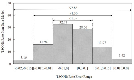
Figure 2.
Basic prediction accuracy of the three machine learning models.
Individual models prior to coupling struggle to optimize performance across all error ranges simultaneously, which limits their overall predictive capability. In contrast, the hybrid model demonstrates improved accuracy and stability compared to any single model. It maintains high precision while reducing prediction errors caused by the inherent limitations of individual algorithms. The multi-model fusion strategy not only enhances the robustness of the prediction system but also provides a solid foundation for achieving more precise control in BOF steelmaking processes.
3. Development of a Kinetic Model for Carbon Oxidation During BOF Blowing
Numerous researchers have proposed various kinetic models for the basic oxygen furnace (BOF) steelmaking process to describe and predict the evolution of carbon content during different stages of blowing. Lin Dong [6] focused on analyzing the rate-limiting steps in the decarburization kinetics. Guo Hanjie [14] presented the fundamental principles of the three-stage decarburization process in textbook literature. Cai Wei [15] investigated the decarburization rate in the late blowing period based on Fick’s first law of diffusion. Lin Wenhui [16] classified kinetic models according to measurement methods, distinguishing between sub-lance models and off-gas analysis models. Ma Dewen [7] developed a multi-zone kinetic model that simultaneously describes the behavior of carbon, silicon, manganese, and phosphorus across three distinct reaction zones in the BOF. Table 8 summarizes several representative kinetic models for carbon evolution.
Table 8.
Summary of kinetic models for carbon element in converter steelmaking.
Existing decarburization kinetic models provide a solid theoretical foundation and technical support for understanding and optimizing the BOF steelmaking process [21]. However, due to the significant challenges in measuring and calculating key parameters at both experimental and theoretical levels, it is particularly important to conduct feasibility analyses by integrating actual operational control parameters [22]. Ma Dewen [7] applied a three-zone kinetic model to simulate the concentration changes in molten metal elements during the blowing process in a 120-ton top-and-bottom combined blowing converter. The model achieved an average prediction deviation of ±0.0058% for the end-point carbon content, validated against actual production data for various steel grades. Despite their theoretical rigor, most existing kinetic models—including those in Table 8—rely on idealized assumptions (e.g., constant mass transfer coefficients, fixed reaction zones, and uniform mixing) and often neglect real-time operational variables such as lance height, oxygen flow rate, and coolant addition patterns. Moreover, many model parameters (e.g., interfacial area, mass transfer coefficients) are either empirically estimated or unmeasurable in practice, limiting their adaptability to dynamic industrial conditions. These limitations hinder direct application in online process control and necessitate model calibration using plant data [23]. Therefore, the decarburization kinetic model proposed by Ma Dewen [7] is selected in this study as the theoretical framework. It serves as the basis for developing a novel approach: by incorporating practical control parameters and iteratively adjusting the model coefficients, we aim to optimize the kinetic sub-models for each reaction zone, thereby enhancing the model’s accuracy and adaptability to real-world operations. The mathematical formulation of the decarburization kinetics is theoretically sound, but key assumptions require critical assessment. The assumption of constant droplet size simplifies interfacial area estimation but overlooks dynamic droplet breakup and coalescence in the turbulent bath, potentially affecting mass transfer predictions. Similarly, equilibrium approximations at reaction interfaces may not hold under rapid blowing conditions, where kinetic disequilibrium is common. While these simplifications are necessary for model tractability, their impact is mitigated in this study by calibrating mass transfer coefficients with plant data and introducing dynamic corrections based on operational parameters such as lance height and oxygen flow rate.
3.1. Kinetic Model of the Decarburization Reaction in Basic Oxygen Furnace (BOF) Steelmaking
In current research, the BOF steelmaking process involves reactions occurring across multiple interfaces. The overall reaction kinetics are closely related to interfacial area, residence time, physicochemical properties of the slag, and droplet generation rate. Based on the distinction between the jet impact zone and the emulsion zone, the total decarburization rate can be expressed as [7]:
where the subscripts iz and em denote the jet impact zone and the emulsion zone, respectively.
3.2. Kinetic Model of the Jet Impact Zone in BOF Decarburization
The oxidation rate of carbon in the jet impact zone can be written as [7]:
where [%C] is the mass percentage of carbon in the molten steel; Aiz is the interfacial reaction area in the jet impact zone (unit: m2); is the mass of molten steel (unit: kg); is the oxygen mass transfer coefficient for carbon in the jet impact zone (unit: m/s).
Furthermore, the oxygen mass transfer coefficient in the jet impact zone can be expressed as follows [7]:
where is the diffusion coefficient of carbon in the metallic droplets (unit: m2/s); ul is the circulation renewal velocity of the molten steel under top-blowing conditions (unit: m/s); Q is the lance gas flow rate (unit: Nm3/h); g is the acceleration due to gravity (unit: m/s2); Hbath is the bath depth (unit: m); rcm is the impact radius (unit: m).
3.3. Kinetic Model of the Emulsion Zone in BOF Decarburization
In the emulsion zone, the oxidation rate of a single moving metal droplet can be described by a mass transfer-controlled rate equation at the steel side, expressed as follows [7]:
where is the mass transfer coefficient of carbon in the emulsion zone (unit: m/s); is the interfacial area of metal droplets in the emulsion (unit: m2); is the mass of the metal droplets in the emulsion (unit: kg);
The penetration theory can be applied to model the mass transfer coefficient for decarburization of moving metal droplets in the slag-metal emulsion. For spherical droplets rising or falling through the slag layer, the contact time between the metal and slag phases can be approximated as the ratio of droplet diameter to its velocity. The mass transfer coefficient on the steel side can then be calculated as [7]:
where is the mass transfer coefficient of carbon in the emulsion zone (unit: m/s); is the diffusion coefficient of carbon in the metallic droplet (unit: m2/s); u is the velocity of the droplet (unit: m/s); d is the average diameter of the metal droplets (unit: m).
3.4. Prediction Accuracy of the Decarburization Kinetic Theoretical Model
To evaluate the predictive capability of the decarburization kinetic theoretical model for carbon content throughout the entire BOF steelmaking process, an empirical analysis was conducted using actual production data from the enterprise described in Section 1. In the kinetic model, the carbon concentration at reaction equilibrium, denoted as [%C]eq, represents the theoretical equilibrium carbon content [24]. However, since the BOF process operates under non-equilibrium conditions and the true equilibrium endpoint is unmeasurable, the measured tapping sample carbon (TSO) content is approximated as the final carbon concentration in the kinetic model.
A random forest-based optimization algorithm was employed to perform global parameter optimization within a search space consisting of 12 key physical and operational parameters, including the average diameter of metal droplets (dp) and the diffusion coefficient of carbon (DC) [25]. The optimal parameter configuration was achieved by minimizing a weighted mean squared error (MSE) objective function.
The 9199 cleaned samples from the training set (see Table 3) were used for parameter calibration and model tuning, while the 2300 samples in the test set were utilized to assess the model’s prediction accuracy.
The decarburization kinetic model involves multiple physical parameters, such as the carbon diffusion coefficient (DC) and oxygen lance nozzle radius (r), as listed in Table 9.
Table 9.
Parameters of the prediction model for carbon removal kinetics.
The predicted TSC (tapping sample carbon before tapping) and TSO carbon contents from the kinetic theoretical model were compared with the corresponding measured values from actual production. The hit rates for TSC and TSO predictions were calculated and are summarized in Table 10 and Table 11, respectively. The corresponding histograms are shown in Figure 3 and Figure 4.
Table 10.
Precision of TSC content hit rate before introducing control parameters.
Table 11.
Precision of TSO carbon content hit rate before introducing control parameters.
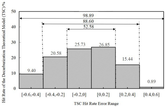
Figure 3.
Prediction accuracy of the TSC kinetic model for carbon before optimization.
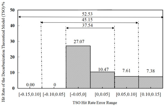
Figure 4.
Prediction accuracy of the TSO kinetic model for carbon before optimization.
The relatively low prediction accuracy, particularly for TSO (only 52.53% within ±0.15%), can be attributed to several simplifications in the base kinetic model. Key operational control factors—such as lance height, oxygen flow rate, and coolant addition timing—are not explicitly incorporated, limiting the model’s responsiveness to real-world process variations. Additionally, unmodeled or oversimplified phenomena, including dynamic slag formation, foaming behavior, and non-uniform mixing, introduce uncertainties in carbon oxidation rates. The assumption of fixed mass transfer coefficients and equilibrium conditions further reduces model adaptability. These limitations highlight the need for model correction using actual control parameters, which is addressed in the subsequent optimization phase.
Analysis of the prediction results reveals that within the error range of [−0.2%, +0.2%], only 52.58% of the TSC samples meet this accuracy criterion. Similarly, for TSO carbon content within the narrower range of [−0.1%, +0.1%], the hit rate is 52.53%, indicating limited performance at high-precision levels. As observed from the histograms, although a majority of the predicted values are clustered near zero error, a significant proportion of data points exhibit relatively large deviations from the measured values. This suggests that introducing additional influencing variables (e.g., dynamic slag formation, temperature evolution) or refining the calibration of existing parameters could help reduce the gap between predicted and actual carbon content, thereby improving the overall prediction accuracy of the kinetic model.
4. Control-Parameter-Integrated Kinetic Model for Decarburization in the BOF Process
Based on practical operational experience, four key control parameters—lance gas flow rate, lance height, hot metal charge mass, and flux addition amount—are known to significantly influence the mass transfer coefficients in the kinetic reactions of element removal during BOF steelmaking [26]. Therefore, to improve the prediction accuracy of the theoretical decarburization kinetic model and enhance its applicability to real-world production conditions, this study integrates these operational control parameters into the existing two-zone decarburization model. This integration enables the model to better reflect actual process dynamics, effectively avoid abnormal operating conditions and product quality issues, and significantly improve production efficiency [27].
4.1. Revised Kinetic Model for the Jet Impact Zone
Fitting analysis of actual plant data reveals that the hot metal charge mass (M0) directly affects the physicochemical characteristics of the molten bath—such as temperature distribution and fluid flow behavior—thereby altering the thickness of the mass transfer boundary layer and the diffusion pathways of elements [28]. As M0 increases, the thermal capacity of the bath rises, leading to changes in jet penetration depth and energy distribution during blowing. To account for this effect, the mass transfer coefficient is dynamically corrected using M0. To enhance model robustness [29] and improve its adaptability to variations in raw material inputs, the hot metal mass M0 is introduced as a scaling factor to quantify the impact of different hot metal batches on mass transfer efficiency.
In addition, during actual operation, lance height (h) is frequently adjusted in response to bath level changes and different blowing stages, significantly influencing the decarburization kinetics. The lance height fundamentally governs the momentum transfer from the oxygen jet to the molten bath, directly affecting the size and stability of the impact crater, emulsion formation, and interfacial area between metal and slag. A higher lance reduces penetration depth, promoting slag foaming and reducing iron oxidation, while a lower lance intensifies jet penetration, enhancing carbon-oxygen reaction rates in the emulsion zone. These hydrodynamic and interfacial effects critically determine the decarburization rate and must be captured in the kinetic model for accurate process representation. Therefore, incorporating the lance height parameter into the kinetic theoretical model is essential. Operators can use real-time lance height measurements to dynamically update model parameters, enabling adaptive simulation across varying operational conditions [30]. The correction functions for M0 and h are formulated in power-law form based on dimensional analysis and analogy to turbulent jet penetration and mass transfer scaling laws in multiphase reactors. The exponents aa and b are determined through regression on industrial data, but their physical interpretability is preserved: a > 0 reflects increased mixing intensity with larger bath mass (up to saturation), while b < 0 aligns with reduced jet penetration and interfacial area at higher lance positions. This semi-empirical approach ensures both model accuracy and consistency with underlying fluid dynamic principles.
By introducing correction factors for calibration, the revised mass transfer coefficient in the jet impact zone is expressed as:
where DC: diffusion coefficient of carbon in metal droplets (unit: m2/s); ul: circulation renewal velocity of molten steel under top-blowing (unit: m/s); Q: lance gas flow rate (unit: Nm3/h); g: gravitational acceleration (unit: m/s2); Hbath: bath depth (unit: m); rcm: impact crater radius (unit: m); M0: hot metal charge mass (unit: kg); a: empirical exponent for hot metal mass correction; :calibration coefficient for the jet impact zone; h: lance height above the bath (unit: m); b: empirical constant for lance height adjustment.
A sensitivity analysis was conducted by varying M0 (±15% around nominal value) and h (±20%) while holding other inputs constant. Results show that a 10% increase in M0 leads to a 6.2% increase, consistent with enhanced bath mixing at larger charges. In contrast, a 10% increase in h by 8.5%, reflecting diminished jet penetration and interfacial area. These trends confirm that the model responds physically to operational changes, with lance height exerting a stronger influence than hot metal mass, which aligns with industrial observation.
4.2. Revised Kinetic Model for the Emulsion Zone
Based on slag-metal reaction thermodynamics and mass transfer principles [31], the lime addition mass (MLime) is introduced as a dynamic correction factor. Lime (CaO), as the primary flux, directly determines the slag basicity (R = CaO/SiO2) [32], which in turn influences key interfacial properties:
Interfacial tension: Lower interfacial tension enhances wettability and increases the effective slag-metal contact area;
Slag viscosity: Reduced viscosity facilitates mass transfer and element diffusion across phases.
By incorporating MLime into the model, the dynamic impact of flux addition on the mass transfer process can be quantified, thereby addressing the discrepancy between the traditional assumption of constant basicity and the actual operational fluctuations observed in industrial practice [33].
Combining analysis of industrial trial data, a revised mass transfer coefficient model considering the synergistic effect of stirring energy is established:
where : mass transfer coefficient of carbon in the emulsion zone (unit: m/s); DC: diffusion coefficient of carbon in the steel phase (unit: m2/s); u: velocity of metal droplets (unit: m/s); d: average diameter of metal droplets (unit: m); MLime: mass of lime flux added (unit: ton); a: empirical exponent for lime addition, used as a calibration parameter.
While MLime serves as a practical proxy for basicity evolution, its effect is implicitly linked to measured or estimated SiO2 content from hot metal analysis, ensuring RR remains within a physically meaningful range. Temperature dependence is accounted for through the temperature-sensitive terms in the base mass transfer coefficient. In industrial applications, real-time temperature measurements (via sub-lance or estimation models) are used to update these parameters dynamically, ensuring the model captures the combined influence of slag chemistry and thermal state on decarburization kinetics.
4.3. Model Parameter Calibration and Accuracy Evaluation
The predicted end-point TSO from a machine learning-coupled model, along with other kinetic parameters, is used as input to the process prediction model. Through continuous comparison with actual BOF operational data, the kinetic model parameters are iteratively optimized, and the prediction accuracy is evaluated.
The iterative algorithm serves as the core of the process simulation, enabling self-adjustment during computation to progressively reduce prediction error. In this study, the forest_minimize function [34] is employed, which uses a random forest-based surrogate model to locate the minimum of the objective function (e.g., weighted mean squared error). The optimization process demonstrates stable convergence, typically reaching a plateau within 150 iterations, with less than 0.5% improvement in the objective function thereafter. Robustness was assessed through 10 independent optimization runs, which yielded consistent optimal parameter sets, with a coefficient of variation (CV) of less than 2% across runs. These results confirm that the algorithm is both convergent and robust under stochastic variations. The 9199 cleaned samples from the training set are used for parameter optimization of the control-parameter-integrated kinetic model, while the 2300 samples in the test set are used to assess the final model accuracy.
Through iterative searching, the optimal parameter set that minimizes the prediction error is identified. Combined with the physical parameters listed in Table 9, Table 12 (presented below) summarizes the calibrated control-parameter-integrated kinetic parameters for each reaction zone, obtained through cyclic fitting of the decarburization kinetic model.
Table 12.
Control parameters of the decarburization kinetics model fusion.
The calibrated parameters in the control-parameter-integrated kinetic model, while optimized using data-driven methods, are not merely empirical fitting constants but carry clear physical and metallurgical significance rooted in the underlying process dynamics. The hot metal charge mass exponent of 0.75 reflects the sub-linear enhancement of mass transfer with increasing bath size, consistent with turbulent jet penetration theory—larger charges improve thermal stability and promote deeper oxygen jet penetration, yet wall effects and reduced relative momentum at excessive masses lead to diminishing returns in mixing efficiency. The lance height coefficient (0.0005) captures the inverse relationship between lance elevation and jet momentum, where higher positions reduce impingement energy, weaken bath agitation, and decrease interfacial reaction area, with the calibrated value aligning with observed reductions in decarburization rate during soft-blowing practices. Similarly, the correction coefficient for the jet impact zone (1.9 × 10⁻⁶) serves as a lumped parameter representing effective surface renewal frequency and boundary layer dynamics under top-blowing conditions, scaling the diffusion-limited flux to match realistic mass transfer intensities observed in high-energy gas-stirred systems. The inclusion of lime addition as a proxy for slag basicity further links operational practice to interfacial phenomena, as increased fluxing lowers slag viscosity and interfacial tension, thereby enhancing slag-metal contact and mass transfer rates. By constructing the correction functions based on dimensional analysis and hydrodynamic scaling laws, the model preserves mechanistic interpretability, ensuring that the optimized parameters represent measurable physical effects—such as mixing intensity, jet penetration depth, and emulsion stability—rather than arbitrary adjustments, thus bridging the gap between theoretical kinetics and industrial operational variability.
The optimized correction parameters obtained from the parameter tuning process are incorporated into the control-parameter-integrated decarburization kinetic model. Equations (8) and (9) below represent the kinetic models for the jet impact zone and emulsion zone during the BOF steelmaking process, respectively.
where M0: hot metal charge mass (unit: t); Q: lance gas flow rate (unit: Nm3/min); h: lance height above the bath (unit: m); MLime: mass of flux added (unit: kg).
To evaluate the predictive capability of the control-parameter-integrated kinetic model, the dual-point hit rate at the mid-blowing stage (TSC, Tapping Sample Carbon before tapping) and at the end-point (TSO, final carbon content) is adopted as the core performance metric. The model’s prediction accuracy is systematically analyzed across different error tolerance bands. Taking a real production heat as an example, the following control parameter values are set: Hot metal charge mass: 220 t, Lance height range: 1.5–1.8 m, Lance flow rate: 282 Nm3/min, Flux addition: 6500 kg. A comparison of the predicted carbon content (mass%) with and without integrated control parameters is presented in Figure 5, with a close-up view of the mid- and end-point regions shown in Figure 6.
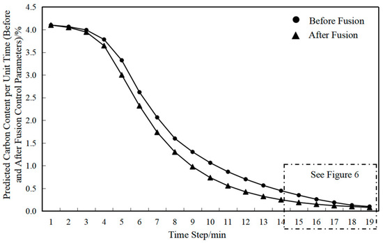
Figure 5.
Unit-time predicted carbon content before and after control parameter integration.
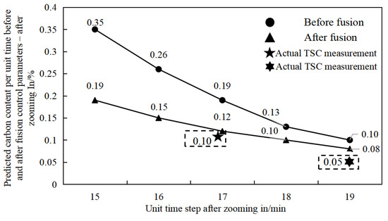
Figure 6.
Localized amplification: pre-and post-control parameter carbon content predictions.
At the TSC (mid-blowing carbon measurement) stage, the prediction error of the decarburization kinetic model with integrated control parameters is reduced by 0.07 wt% compared to the model without parameter integration. At the TSO (end-point carbon measurement) stage, the prediction error is reduced by 0.02 wt%. In the complex and dynamic industrial environment, appropriate parameter adjustment helps overcome the limitations of traditional models and provides more reliable predictions.
To ensure a rigorous evaluation of model performance, an independent validation dataset consisting of 2300 heats from a distinct time period (one month of production data not included in the training phase) was used to assess prediction accuracy. This temporal split ensures no data leakage and provides a realistic assessment of model generalization under industrial operating conditions. The reported hit rates and error reductions for TSC and TSO are computed on this held-out test set, rather than the training or calibration data. Furthermore, the consistency of performance improvements across multiple consecutive validation periods confirms the robustness of the proposed approach.
To evaluate the performance of the optimized model, the predicted TSO and TSC contents from the validation set are compared with actual production data, and the hit rates are calculated based on the absolute deviations. By inputting the actual process parameters for each heat, the hit rates for TSO and TSC before and after optimization are obtained. The comparative results are presented in Figure 7 and Figure 8, respectively.
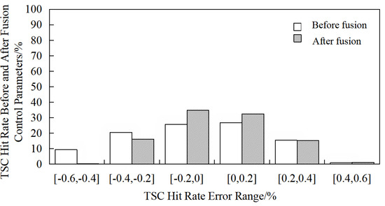
Figure 7.
Comparison of the prediction for the carbon kinetics model (TSC) before and after optimization.
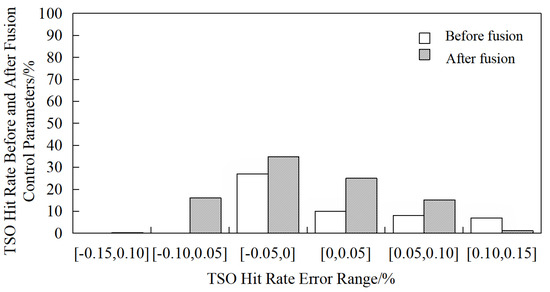
Figure 8.
Comparison of predictions for the carbon kinetics model (TSO) before and after optimization.
The model achieves a 6.26% improvement in TSC hit rate within the error band of [−0.2, +0.2] wt%, and significant improvements in TSO hit rate: 21.30% increase within [−0.05, +0.05] wt%, 19.51% increase within [−0.15, +0.15] wt%. These results demonstrate the model’s enhanced capability in controlling and predicting end-point carbon content. This improvement is attributed to the synergistic optimization of mass transfer coefficients in both the jet impact zone and emulsion zone by the parameter tuning algorithm, particularly through the accurate calibration of the hot metal charge mass exponent and diffusion coefficient.
5. Conclusions
- This study presents a novel approach for integrating controllable operational parameters into the theoretical model for decarburization kinetics prediction. For the first time, adjustable parameters such as hot metal charge mass and flux addition amount are deeply coupled with the kinetic model, overcoming the limitations of traditional models that rely on fixed or averaged input parameters.
- The end-point carbon content (TSO) is predicted by an ensemble of three machine learning models and used as input to the decarburization kinetic model, replacing conventional equilibrium-based assumptions. This strategy captures heat-to-heat variations and better reflects actual production conditions, enabling a closed-loop optimization of the BOF decarburization kinetic model.
- Based on a full year of actual production data from an industrial plant, the proposed model achieves a 6.26% improvement in hit rate for mid-blow carbon (TSC) within the error band of [−0.2, +0.2] wt%, and a 21.30% increase in end-point carbon (TSO) hit rate within [−0.05, +0.05] wt%. These results validate the effectiveness of integrating control parameters in enhancing the accuracy of theoretical decarburization kinetic models. The improved prediction accuracy translates directly into industrial benefits: higher hit rates reduce the need for post-blowing and reblowing, lowering oxygen and energy consumption, decreasing yield loss, and increasing furnace productivity.
Author Contributions
Conceptualization, D.H.; Methodology, K.F., L.Y. and M.Z.; Writing—original draft, K.C. All authors have read and agreed to the published version of the manuscript.
Funding
This research received no external funding.
Data Availability Statement
The original contributions presented in this study are included in the article. Further inquiries can be directed to the corresponding authors.
Conflicts of Interest
Author Meng Zhang was employed by China Metallurgical Industry Planning and Research Institute. The remaining authors declare that the research was conducted in the absence of any commercial or financial relationships that could be construed as a potential conflict of interest.
References
- Cui, B.; Li, J.; Song, S.; Wang, C. Quality molten steel control mixing multi-reaction zone dynamics and off-gas analysis system. Iron Steel 2025, 60, 84–91. [Google Scholar]
- Kim, J.; Cho, M.K.; Jung, M.; Kim, J.; Yoon, Y.S. Rotary hearth furnace for steel solid waste recycling: Mathematical modeling and surrogate-based optimization using industrial-scale yearly operational data. Chem. Eng. J. 2023, 464, 142619. [Google Scholar] [CrossRef]
- Wang, D.; Bao, Y.; Gao, F.; Xing, L. Hybrid Model for Predicting Oxygen Consumption in BOF Steelmaking Process Based on Cluster Analysis. Steel Res. Int. 2022, 94, 2200595. [Google Scholar] [CrossRef]
- Ghalati, M.K.; Zhang, J.; Udu, A.G.; Dong, H. Dynamic Prediction of Reblowing Necessity in BOF Steelmaking. In Proceedings of the 2024 International Conference on Machine Learning and Applications (ICMLA), Miami, FL, USA, 18–20 December 2024; pp. 1924–1927. [Google Scholar]
- Yang, K.J. Development of Static and Kinetic Models for Steelmaking in BOF; Northeastern University: Boston, MA, USA, 2020; pp. 20–31. [Google Scholar]
- Dong, L.; Chenglin, Z.; Guiyu, Z.; Fei, P.; Zongshu, Z. Mechanism Model Steelmaking Process in Combined Blowing Converter. China Metall. 2006, 16, 31–35. [Google Scholar] [CrossRef]
- Ma, D.W.; Li, J.; Song, S.Y.; Ma, D.; Li, J.; Song, S.; Wang, C.; Huang, Y.; Wang, X. Prediction of molten steel composition and temperature based on converter reaction kinetics. Steelmaking 2023, 39, 17–26. [Google Scholar]
- Dogan, N.; Brooks, G.A.; Rhamdhan, M.A. Comprehensive model of oxygen steelmaking Part1: Model development and validation. ISIJ Int. 2011, 51, 1086–1092. [Google Scholar] [CrossRef]
- Lytvynyuk, Y.; Schenk, J.; Hiebler, M.; Sormann, A. Thermodynamic and kinetic model of the converter steelmaking process: The Description of the BOF model. Steel Res. Int. 2014, 85, 537. [Google Scholar] [CrossRef]
- Liu, Y.; Zhang, X.G.; Peng, Q.; Fan, D.; Deng, A.; Xia, Y. Hybrid modeling and multi-network optimization for predicting oxygen supply in converter steelmaking. Chin. J. Process Eng. 2025, 25, 500–509. [Google Scholar]
- Xie, L.Y.; Zhan, D.P.; Lin, Y.K. Endpoint Prediction of Converter Steelmaking based on Backpropagation Neural Network. J. Univ. Sci. Technol. Liaoning 2025, 27, 32–36. [Google Scholar]
- Dong, X.; Han, X.; Yang, X.; He, Z.; Qiao, X.; Zhu, H. A prediction model for dynamic alloy addition after converter based on CNN-LSSVM. Iron Steel 2025, 60, 75–83. [Google Scholar]
- Hong, K.; Zhao, Z.; Zhong, L.; Yu, H.; Liu, C. Development of data driven prediction model for endpoint slag composition and slag splashing time of converter. Steelmaking 2023, 39, 21–27. [Google Scholar]
- Guoh, J. Metallurgical Physical Chemistry Tutorial; Metallurgical Industry Press: Beijing, China, 2006; pp. 80–102. [Google Scholar]
- Cai, W. Basic Theory and Application Research on Predictive Model for Steelmaking Process in Combined Blowing Converter; China Iron and Steel Research Institute: Beijing, China, 2024; pp. 2–6. [Google Scholar]
- Lin, W.H. Study on Process Behavior Analysis and Decarburizaiton Control of BOF Steelmaking; University of Science and Technology Beijing: Beijing, China, 2022; pp. 10–17. [Google Scholar]
- Zhang, Q.; Yang, Y.; Dai, Y.X.; Zhang, Q.; Yang, Y.; Dai, Y.; Lin, L. BOF smelting model based on coupling reaction mechanism. Iron Steel 2024, 59, 40–49. [Google Scholar]
- Rout, B.K.; Brooks, G.; Rhamdhani, M.A.; Li, Z.; Schrama, F.N.H.; Sun, J. Dynamic model of basic oxygen steelmaking process based on multi-zone reaction kinetics: Model derivation and validation. Metall. Mater. Trans. B Process Metall. Mater. Process. Sci. 2018, 49, 537–557. [Google Scholar] [CrossRef]
- Li, P.; Zhan, D.; Wang, B.; Wang, M.; Yang, N. Data-Driven and Mechanistic Hybrid Model for Predicting Oxygen Consumption in BOF Steelmaking. Metall. Mater. Trans. B 2025, 56, 2558–2572. [Google Scholar] [CrossRef]
- Wang, R.B. Hybrid Models for BOF Steelmaking and Continuous Casting Applications. Ph.D. Thesis, McMaster University, Hamilton, ON, Canada, 2022; pp. 2–18. [Google Scholar]
- Cicutti, C.; Poltarak, G.; Ferro, S. Estimation of Internal Cracking Risk in the Continuous Casting of Round Bars. Steel Res. Int. 2017, 88, 20–42. [Google Scholar]
- Wang, X.; Wang, L.; Liu, G.; Mu, W.; Liu, K. Energy balance of BOF converter during swirl-type oxygen lance blowing process. J. Iron Steel Res. Int. 2025, 32, 2744–2756. [Google Scholar] [CrossRef]
- Reynoso, O.A.; Gómez, V.O.; Calderón, R.F.; Vergara-Hernández, H.J.; Herrejón-Escutia, M.; Dávila-Pérez, M.I.; López-Martínez, E. Kinetics of austenite formation during continuous heating in as-cast and as-annealed conditions in a low carbon steel. Mater. Res. Express 2025, 12, 026502. [Google Scholar] [CrossRef]
- Zhang, H.; Zhong, J. Efficient and effective counterfactual explanations for random forests. Expert Syst. Appl. 2025, 293, 128661. [Google Scholar] [CrossRef]
- Rupesh, P.; Murugesan, K. A novel two-zone sequential optimization model for pyro-oxidation and reduction reactions in a downdraft gasifier. RSC Adv. 2023, 13, 9128–9141. [Google Scholar]
- Hewage, K.A.; Rout, K.B.; Brooks, G.; Naser, J. Analysis of steelmaking kinetics from IMPHOS pilot plant data. Ironmak. Steelmak. 2016, 43, 358–370. [Google Scholar] [CrossRef]
- Qian, Q.T. Process Monitoring and Quality Prediction of Basic Oxygen Furnace Steelmaking Process Based on Functional Data Analysis; University of Science and Technology Beijing: Beijing, China, 2023; pp. 5–10. [Google Scholar]
- Zhang, Y.; Zhu, R.; Song, X.; Yang, P. Distributed operational optimization of multi-energy microgrid clusters considering system robustness. Electr. Power Syst. Res. 2025, 248, 111990. [Google Scholar] [CrossRef]
- Wu, C.; Kong, Y. Application of Improved Whale Algorithm to Optimize Dephosphorization Process Parameters in Converter Steelmaking. Appl. Sci. 2025, 15, 4277. [Google Scholar] [CrossRef]
- Yang, Y.; Li, L.; Bao, J.; Sha, J.; Qiao, M.; Tian, J.; Liu, W.; Zhao, Z.; Zhang, Z. Numerical simulation on metallurgical transport phenomena during DC casting of large-size Mg-Gd-Y alloy billet under various magnetic fields. Therm. Sci. Eng. Prog. 2024, 56, 103082. [Google Scholar] [CrossRef]
- Zheng, K.; Wang, W.; Huang, T.; Wang, J.; Chen, X.H.; Xu, R.S. Influence of temperature and slag composition on wetting behavior of titanium-containing blast furnace slag and tuyere coke. J. Iron Steel Res. Int. 2025, 1–10. [Google Scholar] [CrossRef]
- Zhang, K.; Zheng, Z.; Zhang, L.; Liu, Y.; Chen, S. Method for Dynamic Prediction of Oxygen Demand in Steelmaking Process Based on BOF Technology. Processes 2023, 11, 2404. [Google Scholar] [CrossRef]
- Yang, S.C.; Zhong, L.C.; Zhao, Y. Lime Addition Model of Converter Based on Random Forest Algorithm; Northeastern University: Boston, MA, USA; Jianlong Group, Fushun New Iron & Steel Technology Department: Fushun, China, 2022; pp. 90–96. [Google Scholar]
- Li, Q.; Yang, S.Q.; Chen, S.L.; Sun, M.; Lin, J.; Zhang, X.; Liu, Y. Prediction method of endpoint carbon and temperature of converter steelmaking based on adaptive data augmentation. Metall. Ind. Autom. 2025, 49, 64–74. [Google Scholar]


Disclaimer/Publisher’s Note: The statements, opinions and data contained in all publications are solely those of the individual author(s) and contributor(s) and not of MDPI and/or the editor(s). MDPI and/or the editor(s) disclaim responsibility for any injury to people or property resulting from any ideas, methods, instructions or products referred to in the content. |
© 2025 by the authors. Licensee MDPI, Basel, Switzerland. This article is an open access article distributed under the terms and conditions of the Creative Commons Attribution (CC BY) license (https://creativecommons.org/licenses/by/4.0/).