Article

A Deep Reinforcement Advantage Actor-Critic-Based Co-Evolution Algorithm for Energy-Aware Distributed Heterogeneous Flexible Job Shop Scheduling

School of Artificial Intelligence and Computer Science, Jiangnan University, 1800 Li Hu Avenue, Wuxi 214122, China
*
Author to whom correspondence should be addressed.
Processes 2025, 13(1), 95; https://doi.org/10.3390/pr13010095
Submission received: 28 November 2024 / Revised: 19 December 2024 / Accepted: 30 December 2024 / Published: 3 January 2025
(This article belongs to the Section AI-Enabled Process Engineering)

Abstract

:
With the rapid advancement of the manufacturing industry and the widespread implementation of intelligent manufacturing systems, the energy-aware distributed heterogeneous flexible job shop scheduling problem (DHFJSP) has emerged as a critical challenge in optimizing modern production systems. This study introduces an innovative method to reduce both the makespan and the total energy consumption (TEC) in the context of the DHFJSP. A deep reinforcement advantage Actor-Critic-based co-evolution algorithm (DRAACCE) is proposed to address the issue, which leverages the powerful decision-making and perception abilities of the advantage Actor-Critic (AAC) method. The DRAACCE algorithm consists of three main components: First, to ensure a balance between global and local search capabilities, we propose a new co-evolutionary strategy. This enables the algorithm to explore the solution space efficiently while maintaining robust exploration and exploitation. Next, a novel evolution strategy is introduced to improve the algorithm’s convergence rate and solution diversity, ensuring that the search process is both fast and effective. Finally, we integrate deep reinforcement learning with the advantage Actor-Critic framework to select elite solutions, enhancing the optimization process and leading to superior performance in minimizing both TEC and makespan. Extensive experiments validate the effectiveness of the proposed DRAACCE algorithm. The experimental results show that DRAACCE significantly outperforms existing state-of-the-art methods on all 20 instances and a real-world case, achieving better solutions in terms of both makespan and TEC.

1. Introduction

With the rapid development of the manufacturing industry and the increasingly fierce global market competition, enterprises have continuously raised their demands for production efficiency and flexibility. To quickly adapt to market demands and shorten production lead times, components for large-scale equipment are often allocated to multiple factories for simultaneous manufacturing, a process known as distributed manufacturing [1]. Distributed manufacturing enables the production of high-quality products at lower costs and reduced risks [2], which has led to its growing adoption in practice [3].
The distributed flexible job shop scheduling problem (DFJSP) is an extension of HFSP in the distributed manufacturing environment [4]. As a pivotal issue in the realm of distributed manufacturing, DFJSP has garnered significant attention from both academia and industry. Distributed flexible job shop scheduling has been widely applied in industries such as automotive manufacturing, food processing, precision manufacturing and processing, and pharmaceutical production. DFJSP can be elaborated as follows: Multiple jobs need to be processed within factories that are geographically dispersed. Each factory boasts a certain number of interchangeable machines capable of handling the tasks. Each job comprises multiple operations, and each operation can potentially be performed on multiple machines [5]. The scheduling objective, subject to various constraints such as operation sequence, machine capacity, and processing time constraints, is to optimize one or more performance metrics. These metrics typically include makespan, total energy consumption, and overall cost. Due to its complexity and wide range of practical applications, DFJSP is classified as an NP-hard problem, making it difficult to solve using simple analytical methods. As a result, researchers have proposed a variety of approaches to solve the DFJSP, including heuristic algorithms, meta-heuristic algorithms, and intelligent optimization algorithms. Notable methods include tabu search algorithm [6], genetic algorithms [7,8], chemical reaction algorithm [9], differential evolution algorithms [10], and estimation of distribution algorithm [11], among others. Many previous studies have assumed a homogeneous factory environment, where each factory is equipped with identical machines, and each job can be processed on the same set of machines. However, in reality, factories often differ in terms of machine availability, machine processing times, and types of machines used, which leads to a heterogeneous factory environment [12].
Knowledge-driven domain structures have been demonstrated to enhance the convergence of populations [13]. The memetic framework is widely used for its efficiency [14]. However, various studies have demonstrated that the memetic framework struggles with efficiency in solving the DFJSP, especially when multiple objectives are involved. To overcome this limitation, a co-evolutionary framework has been proposed, inspired by the interdependent relationships observed in nature. This approach, much like cooperative evolutionary [15,16], competitive evolutionary [17,18], and memetic evolutionary [19,20] algorithms, is based on parasitic behavior and aims to model the interactions between different components of the system.
Reinforcement learning (RL) is an effective method for learning and controlling complex and uncertain environments. In RL, an agent interacts with its environment to learn a strategy that maximizes cumulative rewards [21,22]. RL comprises five principles: (1) input and output systems; (2) rewards; (3) artificial intelligence environment; (4) Markov Decision Process (MDP); and (5) training and inference [23]. As a widely recognized and foundational RL algorithm, the AAC algorithm combines an Actor network and a Critic network. In policy-based RL, the goal is to directly optimize the policy to maximize rewards. In contrast, value-based reinforcement learning focuses on estimating the value of each state or state–action pair, indirectly determining the optimal policy by selecting the action that yields the highest reward in each state. The AAC algorithm merges these two approaches, enabling the policy (Actor) to be optimized based on feedback from the value function (Critic) [24]. The Actor network generates actions, while the Critic network estimates the state value function or the state–action value function. Ultimately, both networks are trained through a policy gradient algorithm. For the Critic, deep Q-networks (DQNs) can be used to estimate the temporal difference of the action–state value function. Owing to its benefits, the Actor-Critic framework has found widespread application across a range of problems.
In this study, a deep reinforcement advantage Actor-Critic-based co-evolution algorithm (DRAACCE) is proposed to solve the energy-aware DHFJSP. The contributions of this work are summarized as follows.
(1) The study utilizes the DHFJSP in real-world production scheduling contexts, specifically addressing the heterogeneity of factories. It recognizes that each factory may have varying processing times for the same operation, thereby capturing the practical constraints typically encountered in production environments.
(2) A co-evolutionary framework is introduced. In this framework, two populations are used to handle global and local searches. Knowledge acquired from the global search is passed on to the elite population for co-evolution, helping to explore the solution space more efficiently. Furthermore, a linear ranking-based factory selection operator is introduced to address the constraints of heterogeneous factories, ensuring the selection of factories with lower average processing times while also preserving diversity by allowing other factories a chance to be selected.
(3) The study uses dueling DQN to learn the relationship between the solution space and the actions of the operators. Unlike a traditional DQN, which calculates the Q-value for each action separately, a dueling DQN splits the Q-value into two parts: the state-value function V ( s ) , representing the overall value of a state; and the advantage function A ( s , a ) , which quantifies the advantage of each action relative to the state. This decomposition reduces the variance in value estimation, allowing the network to focus on more efficient learning by concentrating on the state’s overall value rather than individual actions. Additionally, by sharing the state-value function, the dueling DQN avoids redundant computations, improving computational efficiency.
(4) The core of the proposed method is the DRAACCE algorithm, which combines the Actor-Critic framework with the co-evolutionary approach. The Actor is responsible for selecting actions and gathering experience data from the environment. The Critic evaluates the value of these actions, offering feedback signals based on the dueling DQN approach. This ensures that the Actor receives more accurate feedback, improving the learning process.
The structure of this paper is as follows: Section 2 introduces related work in recent years. Section 3 introduces the DHFJSP and the MILP model. Section 4 details the proposed method. Experimental results are provided in Section 5. Section 6 concludes the paper and outlines directions for future work.

2. Related Work

To the best of our knowledge, previous studies mainly focused on the distributed job shop scheduling problems in homogeneous factories. De Giovanni and Pezzella [8] were the first to define the DFJSP and introduce an enhanced genetic algorithm to solve it. Ying and Lin [25] proposed the distributed hybrid flow shop scheduling problem with multiprocessor tasks and introduced a self-tuning iterated greedy algorithm to minimize makespan. Shao et al. [26] proposed a multi-neighbor search-based iterated greedy algorithm to address the distributed hybrid flow shop scheduling problem with the objective of minimizing makespan. Chang and Liu [7] presented a hybrid genetic algorithm within a novel encoding mechanism to tackle the DFJSP. Du et al. [11] and Zhang et al. [27] addressed crane transportation constraints in the DFJS. Du employed an optimization algorithm that combines estimation of distribution algorithm and variable neighborhood search, while Zhang applied a Q-learning-based hyper-heuristic evolutionary algorithm.
However, the studies mentioned above assume that all factories are identical, overlooking the differences in factory characteristics. In reality, factories often vary in terms of their manufacturing resources and equipment setups, which results in different processing times for the same job when handled by different factories. Shao et al. [28] studied the distributed heterogeneous hybrid flow shop problem and proposed MOEA based on multi-neighborhood local search. Li et al. [29] proposed an enhanced artificial bee colony (IABC) algorithm that combines simulated annealing with a solution preservation mechanism to improve the solution update process. Wang and Wang [30] introduced a bi-population cooperative memetic algorithm (BCMA), which features a cooperation model based on key factories and localized integration, utilizing several problem-specific neighborhoods to improve the local search. Meng et al. [31] developed three new MILP models, alongside a constraint programming model, to address the problem. However, due to the complexity and challenges of distributed heterogeneous manufacturing systems, research in this area remains limited. Additionally, the growing environmental concerns have led to widespread interest in significantly reducing energy consumption. As a result, researching the energy-aware DHFJSP is of considerable importance. Table 1 presents a comparison of the related work.

3. Problem Description and MILP Model

This section provides a detailed introduction to the DHFJSP and demonstrates the process of assigning workpieces to the corresponding machines in the respective factories for processing. In addition, a MILP model is established for effective mathematical modeling of the DHFJSP.

3.1. Problem Description

In the DHFJSP, there are F heterogeneous factories with diverse manufacturing capabilities. Each factory uses the same set of flexible machines for every operation. However, the processing time for each operation on the same machine in different factories can vary. Each factory possesses m machines within its premises. In factory f ( f = 1 , 2 , , F ) , the machines are represented as M f , k ( k = 1 , 2 , , m ) , each possessing a power consumption E f , k P U .
As shown in Figure 1, n jobs need to be allocated to factories. A job is processed in sequence on a machine within the assigned factory. Once a job is assigned to a factory, it cannot be moved to another, and all its operations must be completed within the same factory. Each job i ( i = 1 , 2 , , n ) consists of o operations. If the operation process O i , j ( j = 1 , 2 , , o ) is handled by machine M f , k , it requires t f , k , i , j time units and consumes E f , k P U × t f , k , i , j energy units. In addition, E f , k S U is usually lower than E f , k P U . The DHFJSP seeks to minimize two objectives: total energy consumption (TEC) and maximum completion time (MCT).

3.2. MILP Model

The Mixed Integer Linear Programming (MILP) model is an optimization technique that represents complex problems using mathematical formulations. In a MILP model, the decision variables can comprise both continuous (real-valued) variables and discrete (integer) variables, while the objective function and all constraint conditions are linear.
The objective of the DHFJSP is to minimize two primary goals: TEC and maximum completion time (MCT). The relevant indices, parameters, and variables involved in the formula are explained in Table 2.
The MILP model of DHFJSP with minimization of TEC and MCT is described as follows:
m i n F 1 = C m a x m i n F 2 = E t o t a l
f = 1 F x f , i = 1 , i
k = 1 m y f , k , i , j = 1 , f , i , j
S i , 1 0 , i
S i , j + 1 S i , j + t f , k , i , j × y f , k , i , j , i , j
S i , j ( S i , j + t f , k , i , j ) + ( 3 y f , k , i , j y f , k , i , j z f , i , i , j ) × U 0 , i i , j , f , k { 1 , 2 , , m j }
z f , i , i , j + z f , i , i , j 1 , f , j , i , i
z f , i , i , j + z f , i , i , j y f , k , i , j + y f , k , i , j 1 , f , j , i > i
C f , i , j = S i , j + f = 1 F k = 1 m y f , k , i , j × t f , k , i , j , f , i , j
C m a x C f , i , j , f , i
E f , k P = i = 1 n y f , k , i , j × E f , k P U × t f , k , i , j , f , j , k { 1 , 2 , , m }
E f , k S = E f , k S U × { max i ( C f , i , j × y f , k , i , j ) min i ( S i , j × y f , k , i , j ) i = 1 n y f , k , i , j × t f , k , i , j } , f , j , k { 1 , 2 , , m }
E t o t a l = f = 1 F j = 1 o k = 1 m ( E f , k S + E f , k P )
x f , i { 0 , 1 } , f , i
y f , k , i , j { 0 , 1 } , f , i , j , k { 1 , 2 , , m }
z f , i , i , j { 0 , 1 } , f , i , i , j
Equation (1) aims to minimize both the maximum completion time and the total energy consumption. Equations (2) and (3) ensure that each job is assigned to exactly one factory and that each operation is processed on only one machine. Inequalities (4) and (5) guarantee that the start time of the first operation for each job is non-negative and that each operation can only begin once the preceding operation of the same job has been completed. Inequalities (6)–(8) ensure that each machine is assigned to only one job at a time. Formulas (9) and (10) define the completion time for each job and the maximum completion time among all jobs, respectively. Formulas (11) and (12) calculate the energy consumption of the machines during processing mode and standby mode, respectively. Formula (13) computes the total energy consumption across all machines, while Formulas (14)–(16) define the binary decision variables.

4. Proposed Algorithm: DRAACCE

This section provides a detailed description of DRAACCE. First, in Section 4.1, the framework of DRAACCE is presented, and the entire process is explained in detail. Next, in Section 4.2, the reasons behind the formation of the DRAACCE framework are discussed, due to the use of the parasitic behavior-based co-evolutionary framework (PCE), and PCE itself is explained in detail. Following that, Section 4.3 provides a detailed introduction to and illustration of the composition of the individuals. The remaining sections describe the various important components of DRAACCE.

4.1. Framework of DRAACCE

The framework of DRAACCE is illustrated in Figure 2. The algorithm begins with a random initialization method. Then, the individuals are sorted in descending order based on their fitness. The co-evolution algorithm is employed to evolve the population, thereby identifying the elite individuals. These elite individuals play a crucial role in guiding the evolution toward promising solution regions by updating the population. To accelerate the convergence speed while maintaining population diversity, DRAACCE uses distinct search strategies for elite and non-elite individuals. Elite individuals undergo further refinement through a combination of neighborhood search, the advantage Actor-Critic network, and an energy-saving strategy to enhance their quality.

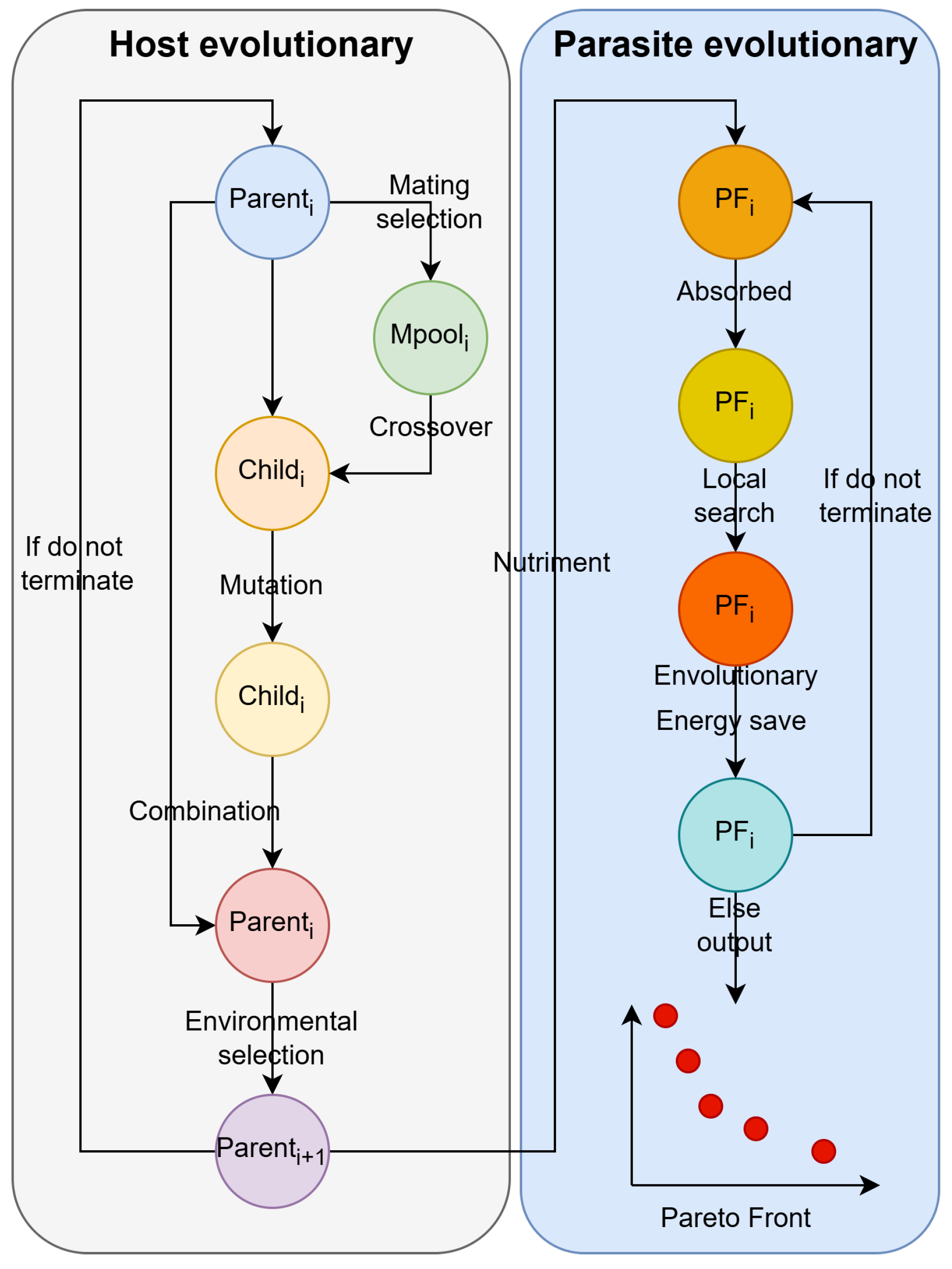
4.2. Parasitic Behavior-Based Co-Evolutionary Framework

The PCE is illustrated in Figure 3. PCE not only determines the framework of DRAACCE but also provides a detailed description of the co-evolution process. To enable the host to thoroughly explore the non-dominated solutions, the framework divides the evolutionary process into two main components: the host H and the parasite P. This division allows for a more dynamic and efficient search for optimal solutions in the scheduling problem. The evolutionary process unfolds in several key stages: Firstly, the host H undergoes one generation using NSGA-II [32]. Secondly, the parasites P absorb Pareto solutions from H. Then, the parasites conduct a local search and AAC network to find more potential non-dominated solutions. Afterwards, the parasites adopt an energy-saving strategy to reduce TEC. Finally, the parasites P produce the ultimate set of non-dominated solutions.
As far as we know, Qin [33] introduced the concept of parasitic cooperative evolution, and Li [34] has already proposed a PCE algorithm for solving multiple optimization benchmarks. However, the algorithm proposed is notably distinct from the PCE presented by Li.
(1) Li’s method employs a tournament selection algorithm for mating selection, where each individual has the same probability to be selected. In contrast, this paper uses linear ranking selection, which ranks individuals based on their fitness from highest to lowest, and the probability of the i-th individual being selected is denoted as P ( i ) , which is calculated using the following equation.
Q ( i ) = a + ( b a ) i 1 p s 1 p s
P ( i ) = Q ( i ) i = 1 p s Q ( i )
where p s represents the total number of individuals, both a and b are constants, and 0 a 1.
(2) During the crossover process, this paper determines the probability of replacing parental genes based on the fitness of the parents, whereas Li’s approach involves random replacement.
(3) Li’s approach uses a precedence operation cross (POX) operation only once on the parent generation to produce two offspring, often resulting in only one valid offspring. In contrast, the approach presented in this paper applies fitness-based POX separately to both parents to generate two offspring. This not only enhances the validity of the generated offspring but also avoids unnecessary offspring from negatively impacting the population.

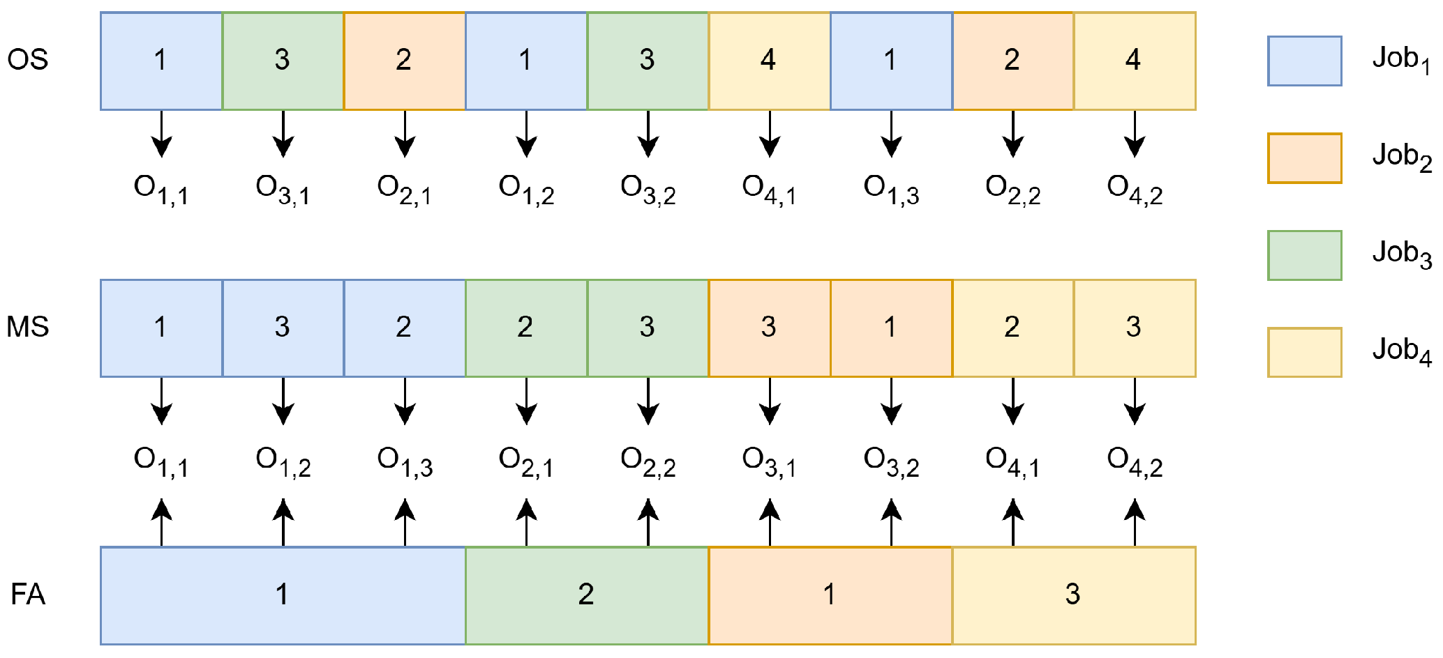
4.3. Encoding Scheme

In the DRAACCE, there are three sub-problems that need to be solved concurrently: determining the processing order for each operation, selecting a factory for each job, and assigning a processing machine to each operation. Therefore, the solution to the problem represented in this work adopts a three-level coding model. Figure 4 illustrates the representation of the solution. The first level is the operation sequence (OS) vector, the second level is the machine selection (MS) vector, and the third level is the factory assignment (FA) vector. The individuals in the DERAACCE algorithm are composed of OS, MS, and FA.
During the decoding process, jobs are allocated to the appropriate heterogeneous factories according to the FA vector. Then, the OS for each factory is retrieved from the OS vector. Subsequently, an optional machine is chosen for each operation based on the MS vector, and the processing time O i , j for that operation can be obtained. Finally, once the machine assignments are made, the starting and finishing times for each operation are computed. From these times, the MCT and TEC for the entire workshop are determined.

4.4. Initialization Population

To achieve significant diversity in the training of the DQN, the algorithm adopts a method of random initialization. Firstly, it randomly generates a sequence of operations. It then randomly chooses a machine from a pool of candidate machines for each operation. Lastly, it randomly assigns each job to a factory.

4.5. Evolution and Environmental Selection

The algorithm employs the POX operator for the OS and adopts the Uniform Crossover (UX) operator for both FA and MS. The evolutionary process of this algorithm is described as follows: (1) Two parent individuals are selected based on linear ranking selection. (2) The two parents undergo the POX and UX operation with a probability of P c , resulting in two offspring. (3) Each offspring undergoes two mutation strategies with a rate of P m : either randomly changing the MS of two operations or randomly selecting two operations and swapping their positions. Then, environmental selection is used to select individuals for the next generation. The environmental selection process is based on the method described in [32].

4.6. Local Search

Local search is a powerful technique for improving the efficiency of evolutionary algorithms by refining existing solutions and accelerating convergence toward optimal or near-optimal solutions. For the DRAACCE algorithm, the local search focuses on identifying more non-dominated solutions in the distributed job shop scheduling problem. The effectiveness of the local search is highly dependent on the selection of key production factors, such as OS, MS, and FA, which play a significant role in determining the solution quality. Therefore, this paper proposes nine local search strategies tailored to the problem characteristics, specifically as follows:
(1) N7: In N7, a block is defined as a sequence of consecutive critical operations that are performed on the same machine along the entire processing path [35]. These operations are considered “critical” because any delay or disruption in their execution can significantly impact the overall schedule. N7 focuses on optimizing the job shop scheduling problem by modifying the operation sequence (OS) within these critical blocks.
(2) Operation Swap: To increase diversity, two operations in the OS from the factory with the highest makespan are randomly swapped.
(3) Critical Operation Swap: Select two critical operations and swap their positions in order to decrease the makespan.
(4) Insert Operation: Randomly select two operations from all the operations from the factory with maximum makespan and insert the latter before the former.
(5) Insert Critical Operation: Randomly select two operations in the critical factory. Then, insert the second operation before the first operation.
(6) Randomly Select Factory Assignment: Randomly pick a job from the critical factory and reassign it to a different factory.
(7) Linear Ranking Factory Assignment: Prior studies have randomly inserted a job into another factory in an attempt to achieve load balancing and reduce completion times [36]. However, the success rate of this random approach was very low. To increase the success rate of reducing makespan, a job is randomly selected from the factory with the maximum makespan and reassigned to a factory that has a shorter average processing time. The probability of each factory being selected is P f , which is calculated using the following equation:
Q f = k = 1 m i = 1 n j = 1 o y f , k , i , j × t f , k , i , j m
P f = Q f f = 1 F Q f
(8) Random Machine Selection: Randomly select a critical operation and assign it to a different available machine within the same factory.
(9) Ranking Machine Selection: Randomly select a critical operation from the machine with the longest processing time and assign it to a machine with a shorter processing time. The probability of each machine being selected is P k , which is calculated using the following equation:
Q k = i = 1 n j = 1 o y f , k , i , j × t f , k , i , j
P k = Q k k = 1 m Q k

4.7. Advantage Actor-Critic-Based Strategy Selection Model

In this paper, we use AAC to choose the most suitable operator. AAC is a powerful deep reinforcement learning algorithm capable of learning data distributions and making correct choices through the analysis of historical experiences. As key components of reinforcement learning, well-designed actions and states can effectively represent the scheduling environment, thereby enhancing the efficiency of the learning process. In this study, a transaction is represented as ( S t , A t , R t , S t + 1 ), where S t is the state, A t is the chosen action, R t is the reward, and  S t + 1 is the subsequent state. S t is a vector formed by combining the OS, MS, and FA. The length of OS and MS corresponds to the total number of operations, while the length of FA corresponds to the number of jobs. A t in AAC consists of the local search actions described in Section 4. The value of R t s given by the following definition: if the old solution is replaced by the new one, R t is 5; if the new solution and the old solution are incomparable, R t is 10; otherwise, R t is 0 [37]. This model inputs state S t into the AAC network and determines the selected action A t based on the ϵ -greedy strategy. By applying action A t to state S t , the next state S t + 1 is generated.
To tackle the challenge of a large and exhaustive state space, AAC utilizes neural networks to learn the distribution of all states within the environment. The AAC algorithm is mainly composed of two key components: the Actor and the Critic. The Actor is a policy network π θ ( S ) responsible for selecting appropriate actions based on the current state. The Critic, on the other hand, is a valuation network V π ( S ) used to evaluate the quality of the policies generated by the Actor. In the Actor-Critic algorithm, there are two update targets: the policy gradient update for the Actor network and the value function update for the Critic network. In AAC algorithm, the Actor network employs the REINFORCE algorithm for gradient updates, while the Critic network adopts the loss function used in DQNs to estimate the temporal difference of the action–state value function for its updates.
In this paper, we will draw inspiration from dueling DQNs for updating the Critic, and divide the Critic into two networks, namely V π 1 ( S ) and T π 2 ( S ) , where V π 1 ( S ) serves as the valuation network and T π 2 ( S ) as the target network. A dueling DQN uses a dual network and introduces the advantage function A ( S , A ) . The action-value function is calculated using the following formula:
Q π ( S , A ) = V π 1 ( S ) + A π 2 ( S , A ) m e a n A A ( S , A )
where π = ( π 1 , π 2 ) . The REINFORCE algorithm is described as follows: At the beginning of training, V π 1 ( S ) and T π 2 ( S ) share the same parameters. Next, randomly select a batch of transactions from the experience pool S. Then, feed the transaction at time t, denoted as S t , into  V π 1 ( S ) , and output the q-values for all actions in the current state as Q π 1 ( S t , : ) . Similarly, input the next state into T π 2 ( S ) and obtain the q-values for the next state Q π 2 ( S t + 1 , : ) . In this paper, the REINFORCE algorithm is used to update the policy gradient, and the formula for this algorithm is as follows:
θ J ( π θ ) = E t [ t = 0 T θ l o g π θ ( A t | S t ) R ( τ ) ]
R ( τ ) = V π 1 ( S t , A t ) R t γ × T π 2 ( S t + 1 , A t + 1 )
where θ J ( π θ ) represents the policy gradient and π θ ( A t | S t ) represents the probability of choosing action A t in state S t . The parameter π 1 is updated using the following loss function:
J ( π 1 ) = 1 2 R 2 ( τ )
where J ( π ) represents the performance of the target policy.
Algorithm 1 illustrates the training part of AAC. By continuously updating π θ and π 1 , we can obtain a better evaluation of the Actor network and improve the selection probability of actions.
Algorithm 1 Training part of advantage Actor-Critic
 1:
Input: Experience pool S, policy network π θ ( S ) , valuation network V π 1 ( S ) , target network T π 2 ( S ) , epochs, counter, maxcount.
 2:
Output: Policy network π θ ( S ) , valuation network V π 1 ( S ) .
 3:
c o u n t = 0
 4:
for  l = 1   t o   e p o c h s   do
 5:
    if  c o u n t e r  %  m a x c o u n t = 0  then
 6:
         T π 2 ( S ) V π 1 ( S )
 7:
    end if
 8:
     c o u n t e r + = 1
 9:
    Random transition ( S t , A t , R t , S t + 1 ) from S
10:
     π θ ( S ) S t
11:
     V π 1 ( S ) ( S t , A t , R t , S t + 1 )
12:
     R ( τ ) T π 2 ( S ) ( S t , A t , R t , S t + 1 )
13:
     θ J ( π θ ) = E t [ t = 0 T θ l o g π θ ( A t | S t ) R ( τ ) ]
14:
     J ( π 1 ) = 1 2 R 2 ( τ )
15:
    Update π θ : π θ = π θ θ J ( π θ )
16:
    Update π 1 : π 1 = π 1 J ( π 1 )
17:
end for

4.8. Energy-Saving Strategy

This paper adopts energy-saving strategies based on fully active scheduling [38]. The detailed description of this strategy is as follows: Firstly, scan the operation sequence forward to identify potential idle slots and insert the current operation O i , j into one of them to reduce idle time. Then, traverse the improved schedule backward to look for positions where the current operation can be inserted to further minimize idle time. This strategy not only reduces TEC but also shortens MCT. The produce of DRAACCE is shown in Algorithm 2.
Algorithm 2 Produce of DRAACCE
 1:
Input: Crossover rate P c , mutation probability P m , learning rate α , discount factory γ , greedy factor ϵ , batch size b s , experience pool size S, epochs, population size p s , update threshold β and MAXNFE.
 2:
Output: The Pareto solutions P S
 3:
Initial host population H, size equals p s
 4:
Initial parasite population P size equals zero
 5:
Initial AAC network: ( π θ , π 1 , π 2 ) ( α , γ , b s , β , S , ϵ )
 6:
N F E = 0
 7:
while  N F E < M A X N F E   do
 8:
    Generate P o o l by linear ranking selection
 9:
    Generate C h i l d by crossover and mutation
10:
    NFE = NFE + | C h i l d |
11:
     U C h i l d H
12:
     H N S G A II ( U )
13:
     P F G e t P a r e t o F r o n t ( H )
14:
     P P F P
15:
     P D e l e t e R e p e a t s o l u t i o n s ( P )
16:
    AAC-based strategies selection:
       [ P , ( π θ , π 1 , π 2 ) ] ( P , ( π θ , π 1 , π 2 ) , ϵ , S )
17:
     N F E = N F E + | P |
18:
     P E n e r g y s a v i n g ( P )
19:
     N F E = N F E + | P |
20:
end while
21:
P S G e t P a r e t o F r o n t ( P )

5. Experimental Evaluation

We designed parameter calibration, ablation, and comparative experiments to evaluate the performance of DRAACCE. Algorithms without AAC were coded in MATLAB 2023, while DRAACCE was coded in Python 3.11 using CUDA 12.0 and PyTorch 1.13.0. The running environment was on a 13th Gen Intel(R) Core(TM) i5-13500H 2.60 GHz with 128 G RAM, and RTX 3090 GPU made by NVIDIA Corporation, located in Santa Clara, CA, USA.

5.1. Instances and Metrics

In this section, Li’s benchmark set [34] is adopted to test the performance of the proposed algorithm. Table 3 presents the parameters of this benchmark and their corresponding values. A total of 20 instances with various scales were generated for testing. The stopping criterion is defined as MAXNEFs = 200 × 1 n n i .
Hypervolume (HV) and Generation Distance (GD) are used to assess the overall performance, convergence, and diversity of multi-objective evolutionary algorithms (MOEAs). Specifically, a lower GD value indicates better convergence of the algorithm, while a higher HV value reflects superior overall performance, as it captures both the quality and diversity of the solution set.

5.2. Parameters Calibration

Since multiple parameters influence the performance of DRAACCE, determining the optimal parameter settings for DRAACCE is crucial. DRAACCE consists of eight parameters and Table 4 presents these parameters and their values. To ensure fairness, each algorithm with different parameter configurations was run 20 times with the same stopping criterion. The average values for all performance metrics across each instance were recorded. Figure 5 and Figure 6 present the main effect plots for the eight parameters relative to the performance indicators. A higher HV value reflects better performance, while better convergence and diversity are indicated by lower GD and Spread values. Table 5 presents the optimal parameter combination for DRAACCE.

5.3. Ablation Experiment

To assess the effectiveness of the various improvements in DRAACCE, eight different algorithms have been designed as follows: (1) Li’s approach: PCE assisted by the DQN (DQCE) [34]; (2) PCE using linear ranking selection assisted by the DQN (DQCE-LR); (3) DQCE with proposed evolution strategy (DQCE-ES); (4) PCE assisted by AAC (AACCE); (5) DQCE-LR with proposed evolution strategy (DQCE-LRES); (6) PCE using linear ranking selection assisted by AAC (AACCE-LR); (7) AACCE with a proposed evolution strategy (AACCE-ES); (8) DRAACCE. To ensure a fair comparison, each algorithm is independently executed 20 times on all instances using the same stopping criterion (MAXNFEs = 200 × 1 n n i ).
Table 6 and Table 7 present the statistical results of all metrics for each variant algorithm. In these tables, the first column contains the basic information for each dataset, where “J” represents jobs and “F” represents factories, so “100J6F” indicates that this dataset has 100 jobs and 6 factories. The symbols “-” and “+” indicate significant inferiority and superiority to DRAACCE, respectively. The symbol “=” denotes no significant difference between the variant algorithm and DRAACCE. Additionally, the best value for each metric is marked in bold. Table 8 displays the results of the Friedman’s rank sum test, with a confidence level of α = 0.05. From the experimental outcomes, the following conclusions can be made. (1) A p-value of less than 0.05 demonstrates that DRAACCE outperforms all variants; and (2) the effectiveness of PCE using linear ranking selection, DQCE with proposed evolution strategy, and AAC can be ensured by analyzing the data in the table.

5.4. Comparison Experiment

To assess the performance of DRAACCE, it is compared with six other algorithms: MOEA/D [39], NSGA-II [32], TS-NSGA-II [40], HSLFA [36], LRVMA [41], and MOEA/D-DQN [37]. Wang et al. [42] proposed a MOEA/D algorithm for energy-efficient scheduling in distributed heterogeneous welding flow shop, demonstrating the effectiveness of MOEA/D in energy-saving DHFJSP. NSGA-II is a classical multi-objective evolutionary algorithm and has been widely applied in the field of the multi-objective flexible job shop scheduling problem. TS-NSGA-II algorithm is a recently proposed algorithm. TS-NSGA-II is divided into two stages: in the first stage, the algorithm primarily uses global search to obtain an initial set of solutions; in the second stage, the algorithm performs local search on the solutions obtained from the first stage to further enhance the convergence and diversity of the solution set. TS-NSGA-II has demonstrated strong performance in solving the multi-objective flexible job shop scheduling problem. Meng et al. developed a new MILP model and proposed a state-of-the-art algorithm, HSLFA, to solve the energy-efficient DFJSP. The LRVMA algorithm is used to solve the multi-objective energy-efficient FJSP with type-2 processing times, considering the minimization of makespan and TEC. DRAACCE fully combines the advantages of the aforementioned six algorithms and effectively avoids their shortcomings.
For a fair comparison, the parameters for the all algorithms are set according to the values provided in their respective references: P c = 1.0, p s = 100 and P m = 0.2. Both MOEA/D-DQN and MOEA/D use a neighborhood size of 10. The reinforcement learning parameters for LRVMA and MOEA/D-DQN are set to match those of DRAACCE. To ensure fairness, all MOEAs incorporate the same local search and energy-saving strategies. Additionally, all comparison algorithms use the same stopping criterion. Each algorithm is run 20 times independently across all instances.
Table 9 and Table 10 list the statistical results for each algorithm. In the final row of each table, the symbols “-/+” indicate that the compared algorithm is significantly inferior or superior to DRAACCE, respectively, while “=” denotes no significant difference between the algorithms. Additionally, the best value for each metric is marked in bold. According to the results in Table 9 and Table 10, DRAACCE significantly outperforms all the compared algorithms in terms of the HV and GD metrics. Table 11 presents the Friedman’s rank sum test results for all algorithms across all instances, with a confidence level of α = 0.05. DRAACCE ranks first in all metrics, with a p-value < 0.05, indicating that DRAACCE is superior to the compared algorithms. Figure 7 shows the Pareto front of all the comparison algorithms on 200J7F. As shown in Figure 7, DRAACCE can find better Pareto solutions than the other comparison algorithms, indicating that the DRAACCE algorithm outperforms the others. In addition, it also shows a conflicting relationship between makespan and TEC, and can roughly reflect the relationship between them. By combining the analysis of the relationship with practical considerations, the Pareto solution that best meets the actual requirements can be identified from the Pareto front.

5.5. Real-World Case

To better assess the effectiveness of DRAACCE, the comparison algorithms are tested using a real-world case [34]. The detailed information of the real-world case can be found in the Appendix A. The algorithms discussed in Section 5.4 are compared with DRAACCE, using the same settings as in the previous section. Table 12 presents the statistical results for each algorithm. The best value is marked in bold. According to the results in Table 12, DRAACCE significantly outperforms all the compared algorithms in terms of the HV and GD metrics in the real-world case. The p-value < 0.05 suggests that DRAACCE outperforms the compared algorithms.

6. Conclusions

This paper presents a deep reinforcement advantage Actor-Critic-based co-evolutionary algorithm for the energy-efficient DHFJSP. First, a PCE using linear ranking selection was proposed to solve the problem. Then, a new evolution strategy was adopted to enhance convergence and diversity. Furthermore, a deep reinforcement learning algorithm AAC with a dueling DQN was used to model the solution distribution and choose the most suitable local search strategy. Finally, the performance of the DRAACCE algorithm in DHFJSP was verified through numerical experiments conducted on 20 instances and a real-world case.
For future work, the following aspects can be considered. First, incorporating an end-to-end network for the DHFJS, which could enhance its generalization ability. Second, extending the model to address the differential DHFJSP, which includes variations in the number of machines, machine failures, or maintenance scenarios, could further improve its robustness and applicability. Finally, researching on dynamic DHFJSP, which includes factors commonly encountered in real-world environments, such as machine failures, emergency order insertion, and maintenance scheduling.

Author Contributions

Conceptualization, H.X., J.T., J.Z. and L.H.; methodology, H.X., J.T. and C.Z.; software, H.X., J.T. and J.Z.; validation, H.X., J.T. and L.H.; formal analysis, J.T. and C.Z.; writing—original draft preparation, H.X. and J.T.; writing—review and editing, L.H., J.Z. and C.Z.; visualization, H.X. and J.T.; supervision, L.H., J.Z. and C.Z.; project administration, H.X. All authors have read and agreed to the published version of the manuscript.

Funding

This research received no external funding.

Data Availability Statement

The code in this article cannot be published due to privacy, and can be obtained from the corresponding author upon reasonable request.

Conflicts of Interest

The authors declare no conflicts of interest.

Appendix A

The real-world case describes the model stamping workshop provided by a large equipment company’s factory in China. The material feeding system converts steel into parts of different sizes for processing in the subsequent machining workshop. Batch orders are considered a basic processing operation and there are three steps to process a batch: cutting, clamping, and bevel cutting. However, due to business confidentiality, the processing data for each stage are not provided, and each operation only includes a single integer operation called blanking. In the real-world case, there are 55 jobs, each with two characteristics: weight and difficulty coefficient. Additionally, in this scenario, there are two factories, each with four worker teams. Each team operates one machine, and the teams have different capabilities (tons of steel processed per hour weight). The processing time for each job can be calculated using the formula: w e i g h t × c o e f f i c i e n t × 1000 / c a p a c i t y . Therefore, the processing time for each operation is different for each team. Additionally, each team of workers can handle all the jobs. Our goal is to minimize the MCT and TEC in this real-world case. Thus, the case is formulated as DHFJSP. The detailed information can be found in Table A1 and Table A2.
Table A1. Details of all the jobs in the real-world case.
Job Index12345
weight0.6680.49122.6660.4938.306
difficulty10.810.70.7
Job Index678910
weight2.5373.3380.2050.2051.958
difficulty0.70.8111
Job Index1112131415
weight10.85510.96141.3172.0183.802
difficulty11111
Job Index1617181920
weight2.0652.2552.3551.4750.585
difficulty11111
Job Index2122232425
weight0.1625.0093.7330.98118.799
difficulty10.810.80.8
Job Index2627282930
weight2.0290.298549.816
difficulty11111
Job Index3132333435
weight0.4261.3630.5434.514.798
difficulty1110.80.8
Job Index3637383940
weight0.6070.43510.1590.159
difficulty0.80.80.811
Job Index4142434445
weight0.2670.37110.5590.3480.311
difficulty110.811
Job Index4647484950
weight10.6490.348742.122
difficulty11111
Job Index5152535455
weight3.3360.2362.7860.8930.286
difficulty11111
Table A2. Details of all the groups in the real-world case.
Group IndexCapacities/KG/hWorker NumberWork Time/Day
G1 in factory174.6 KG/h138 h/d
G2 in factory176.1 KG/h16
G3 in factory180.4 KG/h14
G4 in factory180.9 KG/h17
G1 in factory280 KG/h14
G2 in factory278 KG/h15
G3 in factory279 KG/h14
G4 in factory278 KG/h15

References

  1. Zhang, G.; Wang, L.; Xing, K. Dual-Space Co-Evolutionary Memetic Algorithm for Scheduling Hybrid Differentiation Flowshop with Limited Buffer Constraints. IEEE Trans. Syst. Man Cybern. Syst. 2022, 52, 6822–6836. [Google Scholar] [CrossRef]
  2. Rifai, A.P.; Nguyen, H.T.; Dawal, S.Z.M. Multi-objective adaptive large neighborhood search for distributed reentrant permutation flow shop scheduling. Appl. Soft Comput. 2016, 40, 42–57. [Google Scholar] [CrossRef]
  3. Shih-Wei Lin, K.C.Y.; Huang, C.Y. Minimising makespan in distributed permutation flowshops using a modified iterated greedy algorithm. Int. J. Prod. Res. 2013, 51, 5029–5038. [Google Scholar] [CrossRef]
  4. Pan, Z.; Lei, D.; Wang, L. A Bi-Population Evolutionary Algorithm with Feedback for Energy-Efficient Fuzzy Flexible Job Shop Scheduling. IEEE Trans. Syst. Man Cybern.-Syst. 2022, 52, 5295–5307. [Google Scholar] [CrossRef]
  5. Meng, L.; Zhang, C.; Ren, Y.; Zhang, B.; Lv, C. Mixed-integer linear programming and constraint programming formulations for solving distributed flexible job shop scheduling problem. Comput. Ind. Eng. 2020, 142, 106347. [Google Scholar] [CrossRef]
  6. Xu, W.; Hu, Y.; Luo, W.; Wang, L.; Wu, R. A multi-objective scheduling method for distributed and flexible job shop based on hybrid genetic algorithm and tabu search considering operation outsourcing and carbon emission. Comput. Ind. Eng. 2021, 157, 107318. [Google Scholar] [CrossRef]
  7. Chang, H.C.; Liu, T.K. Optimisation of distributed manufacturing flexible job shop scheduling by using hybrid genetic algorithms. J. Intell. Manuf. 2017, 28, 1973–1986. [Google Scholar] [CrossRef]
  8. De Giovanni, L.; Pezzella, F. An Improved Genetic Algorithm for the Distributed and Flexible Job-shop Scheduling problem. Eur. J. Oper. Res. 2010, 200, 395–408. [Google Scholar] [CrossRef]
  9. Marzouki, B.; Driss, O.B.; Ghedira, K. Solving Distributed and Flexible Job shop Scheduling Problem using a Chemical Reaction Optimization metaheuristic. Procedia Comput. Sci. 2018, 126, 1424–1433. [Google Scholar] [CrossRef]
  10. Wu, X.; Liu, X. An Improved Differential Evolution Algorithm for Solving a Distributed Flexible Job Shop Scheduling Problem. In Proceedings of the 2018 IEEE 14th International Conference on Automation Science and Engineering (Case), Munich, Germany, 20–24 August 2018. [Google Scholar]
  11. Du, Y.; Li, J.q.; Luo, C.; Meng, L.l. A hybrid estimation of distribution algorithm for distributed flexible job shop scheduling with crane transportations. Swarm Evol. Comput. 2021, 62, 100861. [Google Scholar] [CrossRef]
  12. Lu, C.; Gao, L.; Yi, J.; Li, X. Energy-Efficient Scheduling of Distributed Flow Shop with Heterogeneous Factories: A Real-World Case From Automobile Industry in China. IEEE Trans. Ind. Inform. 2021, 17, 6687–6696. [Google Scholar] [CrossRef]
  13. Peng, K.; Deng, X.; Zhang, C.; Pan, Q.K.; Ren, L.; Pang, X. An improved imperialist competitive algorithm for hybrid flowshop rescheduling in steelmaking-refining-continuous casting process. Meas. Control 2020, 53, 1920–1928. [Google Scholar] [CrossRef]
  14. Li, R.; Gong, W.; Lu, C. Self-adaptive multi-objective evolutionary algorithm for flexible job shop scheduling with fuzzy processing time. Comput. Ind. Eng. 2022, 168, 108099. [Google Scholar] [CrossRef]
  15. Ma, X.; Li, X.; Zhang, Q.; Tang, K.; Liang, Z.; Xie, W.; Zhu, Z. A Survey on Cooperative Co-Evolutionary Algorithms. IEEE Trans. Evol. Comput. 2019, 23, 421–441. [Google Scholar] [CrossRef]
  16. Miguel Antonio, L.; Coello Coello, C.A. Coevolutionary Multiobjective Evolutionary Algorithms: Survey of the State-of-the-Art. IEEE Trans. Evol. Comput. 2018, 22, 851–865. [Google Scholar] [CrossRef]
  17. Wang, X.; Zhang, K.; Wang, J.; Jin, Y. An Enhanced Competitive Swarm Optimizer with Strongly Convex Sparse Operator for Large-Scale Multiobjective Optimization. IEEE Trans. Evol. Comput. 2022, 26, 859–871. [Google Scholar] [CrossRef]
  18. Tian, Y.; Zheng, X.; Zhang, X.; Jin, Y. Efficient Large-Scale Multiobjective Optimization Based on a Competitive Swarm Optimizer. IEEE Trans. Cybern. 2020, 50, 3696–3708. [Google Scholar] [CrossRef] [PubMed]
  19. Ong, Y.S.; Lim, M.H.; Chen, X. Memetic Computation-Past, Present & Future. IEEE Comput. Intell. Mag. 2010, 5, 24–31. [Google Scholar] [CrossRef]
  20. Wang, J.; Ren, W.; Zhang, Z.; Huang, H.; Zhou, Y. A Hybrid Multiobjective Memetic Algorithm for Multiobjective Periodic Vehicle Routing Problem with Time Windows. IEEE Trans. Syst. Man Cybern.-Syst. 2020, 50, 4732–4745. [Google Scholar] [CrossRef]
  21. Chen, R.; Yang, B.; Li, S.; Wang, S. A self-learning genetic algorithm based on reinforcement learning for flexible job-shop scheduling problem. Comput. Ind. Eng. 2020, 149, 106778. [Google Scholar] [CrossRef]
  22. Shao, Z.; Pi, D.; Shao, W. Hybrid enhanced discrete fruit fly optimization algorithm for scheduling blocking flow-shop in distributed environment. Expert Syst. Appl. 2020, 145, 113147. [Google Scholar] [CrossRef]
  23. Zhao, F.; Di, S.; Wang, L. A Hyperheuristic with Q-Learning for the Multiobjective Energy-Efficient Distributed Blocking Flow Shop Scheduling Problem. IEEE Trans. Cybern. 2023, 53, 3337–3350. [Google Scholar] [CrossRef]
  24. Zheng, J.; Kurt, M.N.; Wang, X. Stochastic Integrated ActorCritic for Deep Reinforcement Learning. IEEE Trans. Neural Netw. Learn. Syst. 2024, 35, 6654–6666. [Google Scholar] [CrossRef]
  25. Ying, K.C.; Lin, S.W. Minimizing makespan for the distributed hybrid flowshop scheduling problem with multiprocessor tasks. Expert Syst. Appl. 2018, 92, 132–141. [Google Scholar] [CrossRef]
  26. Shao, W.; Shao, Z.; Pi, D. Modeling and multi-neighborhood iterated greedy algorithm for distributed hybrid flow shop scheduling problem. Knowl.-Based Syst. 2020, 194, 105527. [Google Scholar] [CrossRef]
  27. Zhang, Z.Q.; Wu, F.C.; Qian, B.; Hu, R.; Wang, L.; Jin, H.P. A Q-learning-based hyper-heuristic evolutionary algorithm for the distributed flexible job-shop scheduling problem with crane transportation. Expert Syst. Appl. 2023, 234, 121050. [Google Scholar] [CrossRef]
  28. Shao, W.; Shao, Z.; Pi, D. An Ant Colony Optimization Behavior-Based MOEA/D for Distributed Heterogeneous Hybrid Flow Shop Scheduling Problem Under Nonidentical Time-of-Use Electricity Tariffs. IEEE Trans. Autom. Sci. Eng. 2022, 19, 3379–3394. [Google Scholar] [CrossRef]
  29. Li, Y.; Li, X.; Gao, L.; Zhang, B.; Pan, Q.K.; Tasgetiren, M.F.; Meng, L. A discrete artificial bee colony algorithm for distributed hybrid flowshop scheduling problem with sequence-dependent setup times. Int. J. Prod. Res. 2021, 59, 3880–3899. [Google Scholar] [CrossRef]
  30. Wang, J.J.; Wang, L. A Bi-Population Cooperative Memetic Algorithm for Distributed Hybrid Flow-Shop Scheduling. IEEE Trans. Emerg. Top. Comput. Intell. 2021, 5, 947–961. [Google Scholar] [CrossRef]
  31. Meng, L.; Gao, K.; Ren, Y.; Zhang, B.; Sang, H.; Zhang, C. Novel MILP and CP models for distributed hybrid flowshop scheduling problem with sequence-dependent setup times. Swarm Evol. Comput. 2022, 71, 101058. [Google Scholar] [CrossRef]
  32. Deb, K.; Pratap, A.; Agarwal, S.; Meyarivan, T. A fast and elitist multiobjective genetic algorithm: NSGA-II. IEEE Trans. Evol. Comput. 2002, 6, 182–197. [Google Scholar] [CrossRef]
  33. Qin, Q.; Cheng, S.; Zhang, Q.; Li, L.; Shi, Y. Biomimicry of parasitic behavior in a coevolutionary particle swarm optimization algorithm for global optimization. Appl. Soft Comput. 2015, 32, 224–240. [Google Scholar] [CrossRef]
  34. Li, R.; Gong, W.; Wang, L.; Lu, C.; Dong, C. Co-Evolution with Deep Reinforcement Learning for Energy-Aware Distributed Heterogeneous Flexible Job Shop Scheduling. IEEE Trans. Syst. Man Cybern.-Syst. 2024, 54, 201–211. [Google Scholar] [CrossRef]
  35. Zhang, C.; Li, P.; Guan, Z.; Rao, Y. A tabu search algorithm with a new neighborhood structure for the job shop scheduling problem. Comput. Oper. Res. 2007, 34, 3229–3242. [Google Scholar] [CrossRef]
  36. Meng, L.; Ren, Y.; Zhang, B.; Li, J.Q.; Sang, H.; Zhang, C. MILP Modeling and Optimization of Energy- Efficient Distributed Flexible Job Shop Scheduling Problem. IEEE Access 2020, 8, 191191–191203. [Google Scholar] [CrossRef]
  37. Tian, Y.; Li, X.; Ma, H.; Zhang, X.; Tan, K.C.; Jin, Y. Deep Reinforcement Learning Based Adaptive Operator Selection for Evolutionary Multi-Objective Optimization. IEEE Trans. Emerg. Top. Comput. Intell. 2023, 7, 1051–1064. [Google Scholar] [CrossRef]
  38. Li, R.; Gong, W.; Wang, L.; Lu, C.; Zhuang, X. Surprisingly Popular-Based Adaptive Memetic Algorithm for Energy-Efficient Distributed Flexible Job Shop Scheduling. IEEE Trans. Cybern. 2023, 53, 8013–8023. [Google Scholar] [CrossRef]
  39. Zhang, Q.; Li, H. MOEA/D: A multiobjective evolutionary algorithm based on decomposition. IEEE Trans. Evol. Comput. 2007, 11, 712–731. [Google Scholar] [CrossRef]
  40. Ming, F.; Gong, W.; Wang, L. A Two-Stage Evolutionary Algorithm with Balanced Convergence and Diversity for Many-Objective Optimization. IEEE Trans. Syst. Man Cybern.-Syst. 2022, 52, 6222–6234. [Google Scholar] [CrossRef]
  41. Li, R.; Gong, W.; Lu, C.; Wang, L. A Learning-Based Memetic Algorithm for Energy-Efficient Flexible Job-Shop Scheduling with Type-2 Fuzzy Processing Time. IEEE Trans. Evol. Comput. 2023, 27, 610–620. [Google Scholar] [CrossRef]
  42. Wang, G.; Li, X.; Gao, L.; Li, P. Energy-efficient distributed heterogeneous welding flow shop scheduling problem using a modified MOEA/D. Swarm Evol. Comput. 2021, 62, 100858. [Google Scholar] [CrossRef]
Figure 1. Example of distributed heterogeneous flexible job shop.
Processes 13 00095 g001
Figure 2. Framework of DRAACCE.
Processes 13 00095 g002
Figure 3. PCE applied to distributed job shop scheduling.
Processes 13 00095 g003
Figure 4. Solution representation for DRAACCE.
Processes 13 00095 g004
Figure 5. Main effect for HV metrics.
Processes 13 00095 g005
Figure 6. Main effect for GD metrics.
Processes 13 00095 g006
Figure 7. Approximate Pareto front found by each algorithm on 200J7F.
Processes 13 00095 g007
Table 1. Comparison of related work.
ProblemReferenceObjectivesAlgorithmCharacteristics of Model
DFJSPDe Giovanni and Pezzella [8]makespanenhanced genetic algorithmhomogeneous
DHFSPYing and Lin [25]makespanIGAhomogeneous
DHFSPShao et al. [26]makespan and TECmulti-neighbor search-based IGAhomogeneous
DFJSPChang and Liu [7]makespanhybrid genetic algorithmhomogeneous
DFJSPDu et al. [11]makespanoptimization algorithmhomogeneous
DFJSPZhang et al. [27]makespanQHHEAhomogeneous
DHHFSPShao et al. [28]makespanMOEA based on multi-neighborhood local searchheterogeneous
DHHFSPLi et al. [29]makespanIABCheterogeneous
DHHFSPWang and Wang [30]makespanBCMAheterogeneous
DHFJSPThis workmakespan and TECDRAACCEheterogeneous
Table 2. List of indices, parameters, and variables.
TypeSymbolDefinition
IndexiIndex of job, i = 1 , 2 , , n
jIndex of operation, j = 1 , 2 , , o
fIndex of factory, f = 1 , 2 , , F
kIndex of machine, k = 1 , 2 , , m
ParameternNumber of jobs
oNumber of operations for each job
FNumber of factories
mNumber of machines in each factory
M f , k The kth machine in factory f
O i , j The jth operation of the ith job
t f , k , i , j The time units taken by machine M f , k to process operation O i , j
E f , k P U The power consumption of the machine M f , k in processing mode per unit time
E f , k S U The power consumption of the machine M f , k in standby mode per unit time
Variable E f , k P Energy consumption of the machine M f , k in processing mode
E f , k S Energy consumption of the machine M f , k in standby mode
S i , j The start processing time of operation O i , j
C f , i , j The completion time of operation O i , j in the fth factory
C m a x Maximum completion time
x f , i 1 if job i is assigned in factory f, and 0 otherwise
y f , k , i , j 1 if O i , j is processed by machine M f , k , and 0 otherwise
z f , i , i , j 1 if O i , j is processed before O i , j in factory f, and 0 otherwise
Table 3. Parameters of the benchmark and their values.
ParameterValue
Number of jobs10, 20, 30, 40, 50, 100, 150, 200
Number of factories2, 3, 4, 5, 6, 7
Number of machines in each factory5
Number of operations in each job5
Processing time for each operation in each factory[5, 20]
Processing power consumption value4.0 kWh
Standby power consumption value1.0 kWh
Table 4. Parameters of DRAACCE and their values.
ParameterValue
Crossover rate P c 0.8, 0.9, 1.0
Population size p s 100, 150, 200
Mutation rate P m 0.1, 0.15, 0.2
Learning rate α 0.001, 0.005, 0.01
Batch size b s 8, 16, 32
Greedy factor ϵ 0.9, 0.925, 0.95
Discount factor γ 0.9, 0.925, 0.95
Experience replay buffer size S E 512, 768, 1024
Table 5. Optimal parameter combination for DRAACCE.
ParameterValue
Crossover rate P c 1.0
Population size p s 100
Mutation rate P m 0.2
Learning rate α 0.001
Batch size b s 16
Greedy factor ϵ 0.9
Discount factor γ 0.9
Experience replay buffer size S E 512
Table 6. Statistical performance of HV metrics for each variant algorithm across all instances.
InsDQCEDQCE-LRDQCE-ESAACCEDQCE-LRESAACCE-LRAACCE-ESDRAACCE
10J2F0.931-1.286=0.862-0.868-0.807-0.888-0.965-1.256
20J2F0.077-0.849-1.196-1.194-0.861-1.214-0.574-1.562
20J3F0.125-0.727-0.620-0.431-0.717-1.040-0.765-1.733
30J2F0.512-1.108=0.694-0.484-0.717-0.610-0.756-1.225
30J3F0.062-0.624-1.043-1.307=1.324=1.294=1.224=1.334
40J2F0.527-0.772-0.143-0.520-0.747-1.056-1.423-2.462
40J3F0.774-0.801-0.902-0.892-1.418-1.417-0.678-2.164
40J4F0.730-1.485-2.495-2.230-2.072-2.257-2.652-4.002
50J3F0.884-0.687-1.412=0.459-0.558-0.798-0.400-1.400
50J4F0.633-1.070-1.332-1.116-1.226-1.771-1.299-2.751
50J5F0.308-0.098-0.391-0.372-0.041-0.564=0.381-0.698
100J4F0.556-0.509-0.631=0.499-0.669=0.039-0.568-0.738
100J5F0.262-0.773=0.247-0.171-0.770=0.553-0.487-0.766
100J6F0.803-1.202-1.217-1.197-1.218-1.871=1.375-1.772
100J7F0.823-1.041-1.080-1.202-0.637-1.205-1.191-2.667
150J5F0.780-1.240-1.260-1.221-1.116-0.530-1.434=1.606
150J6F1.005-1.163-0.665-1.221-1.387-1.350-1.322-1.617
150J7F0.054-0.264-0.878=0.829=0.844=0.277-0.560-0.820
200J6F0.824-1.968-1.221-1.616-3.702-2.964-2.151-3.909
200J7F0.328-2.302-1.385-3.910-4.573-3.942-5.042-5.725
-/=/+20/0/017/3/017/3/018/2/016/4/017/3/018/2/0
Table 7. Statistical performance of GD metrics for each variant algorithm across all instances.
InsDQCEDQCE-LRDQCE-ESAACCEDQCE-LRESAACCE-LRAACCE-ESDRAACCE
10J2F0.593-0.271=0.449-0.259=0.242=0.488-0.268=0.224
20J2F0.777-0.626-0.611-0.726-0.730-0.697-0.620-0.405
20J3F0.724-0.703-0.815-0.537=0.670=0.582=0.809-0.487
30J2F0.990-0.720-0.554-0.453-0.439-0.239=0.543-0.216
30J3F0.939-0.766-0.726-0.899-0.887-0.821-0.731-0.527
40J2F1.581-1.301-0.883-0.877-0.735=0.936-0.768=0.670
40J3F1.490-1.233-1.452-1.310-1.428-0.810=0.793=0.764
40J4F1.562-1.231-1.339-1.242-1.343-0.876-1.305-0.620
50J3F1.346-1.208-1.079-1.264-0.908-0.977-1.025-0.603
50J4F1.325-1.415-0.767=1.116-1.226-1.771-1.299-0.767
50J5F2.617-2.465-2.249-2.735-1.762-1.307=1.211=1.336
100J4F2.898-2.807-2.793-2.508-1.948-1.169=1.020=1.124
100J5F2.722-2.231-2.111-2.541-2.243-2.317-2.050-1.801
100J6F3.212-2.502-3.226-3.123-2.897-2.806-2.574-2.223
100J7F4.386-3.751-3.620-4.251-2.811-2.254-2.415-1.567
150J5F3.656-3.593-3.549-3.338-3.411-3.337-3.763-2.421
150J6F5.249-4.702-3.315-3.446-3.289-3.777-2.325-2.110
150J7F4.682-4.630-4.214-3.139-3.394-4.009-3.634-2.611
200J6F9.311-4.502-3.839-3.244=4.176-3.948-3.888-3.235
200J7F8.966-4.193-3.206-5.182-3.928-4.499-3.035-2.818
-/=/+20/0/019/1/019/1/017/3/017/3/015/5/015/5/0
Table 8. Rankings from Friedman rank sum test for variant algorithms ( α = 0.05).
MOEAsHV GD
Rankp-ValueRankp-Value
DQCE6.55 8.95 × 10 10 7.55 9.24 × 10 15
DQCE-LR5.306.00
DQCE-ES4.854.85
AACCE5.454.80
DQCE-LRES4.354.15
AACCE-LR3.753.85
AACCE-ES4.303.65
DRAACCE1.351.15
Table 9. Statistical performance of HV metrics for each comparison algorithm across all instances.
InsNSGA-IIMOEA/DTS-NSGA-IIHSLFALRVMAMOEA/D-DQNDRAACCE
10J2F1.126-1.237-1.125-1.154-1.273-1.012-1.829
20J2F1.038-1.272-1.131-1.154-1.258-0.996-1.538
20J3F1.263-1.484-1.352-1.327-1.473-1.174-2.153
30J2F1.026-1.147-1.083-1.059-1.075-0.947-1.827
30J3F1.047-1.253-1.173-1.248-1.241-1.038-2.157
40J2F0.947-1.048-0.989-0.968-1.026-0.875-2.206
40J3F1.126-1.238-1.373-1.341-1.164-1.074-1.985
40J4F1.052-1.241-1.172-1.218-1.283-0.973-1.967
50J3F1.042-1.148-1.083-1.153-1.196-0.952-2.658
50J4F1.182-1.305-1.282-1.235-1.381-1.016-2.386
50J5F1.391-1.572-1.431-1.389-1.528-1.218-2.879
100J4F0.934-1.054-1.058-1.135-1.058-0.852-1.938
100J5F0.792-0.941-0.902-0.872-0.982-0.681-1.763
100J6F0.874-1.027-0.947-0.967-1.027-0.769-1.876
100J7F0.969-1.107-1.080-1.101-1.181-0.942-1.790
150J5F1.092-1.298-1.168-1.198-1.307-0.984-1.870
150J6F1.128-1.337-1.253-1.232-1.374-1.072-2.224
150J7F1.087-1.237-1.158-1.143-1.298-1.102-2.198
200J6F0.931-1.209-1.174-1.144-1.252-0.874-1.889
200J7F0.982-1.103-0.988-0.982-1.138-0.865-1.776
-/=/+20/0/020/0/020/0/020/0/020/0/020/0/0
Table 10. Statistical performance of GD metrics for each comparison algorithm across all instances.
InsNSGA-IIMOEA/DTS-NSGA-IIHSLFALRVMAMOEA/D-DQNDRAACCE
10J2F0.883-0.679-0.839-0.847-0.749-1.039-0.292
20J2F0.980-0.732-0.835-0.948-0.539-1.129-0.347
20J3F1.498-1.173-1.234-1.367-0.985-1.642-0.558
30J2F1.377-1.112-1.322-1.402-1.209-1.531-0.883
30J3F1.076-0.912-1.027-1.073-0.884-1.223-0.667
40J2F0.855-0.875-0.860-0.828-0.999-1.117-0.483
40J3F1.165-0.998-1.055-1.093-0.836-1.336-0.583
40J4F1.257-1.231-1.338-1.365-1.267-1.558-0.895
50J3F1.375-1.127-1.264-1.326-1.268-1.587-0.689
50J4F1.645-1.364-1.484-1.536-1.245-1.976-0.870
50J5F1.458-1.247-1.386-1.405-1.253-1.758-0.689
100J4F1.503-1.284-1.358-1.412-1.063-1.795-0.754
100J5F1.458-1.186-1.372-1.407-1.093-1.658-0.693
100J6F1.648-1.264-1.375-1.462-1.104-2.034-0.859
100J7F1.589-1.134-1.462-1.385-1.087-2.039-0.826
150J5F1.385-1.103-1.273-1.337-0.936-1.847-0.582
150J6F1.573-1.161-1.231-1.315-0.885-1.739-0.483
150J7F1.448-1.128-1.375-1.426-0.864-1.758-0.539
200J6F1.257-0.974-1.184-1.224-0.792-1.663-0.448
200J7F1.570-1.237-1.446-1.428-1.038-2.004-0.836
-/=/+20/0/020/0/020/0/020/0/020/0/020/0/0
Table 11. Rankings from Friedman rank sum test for comparison algorithms ( α = 0.05).
MOEAsHV GD
Rankp-ValueRankp-Value
NSGA-II5.75 7.65 × 10 20 5.65 1.03 × 10 20
MOEA/D2.902.85
TS-NSGA-II4.354.10
HSLFA4.354.85
LRVMA2.702.55
MOEA/D-DQN6.957.00
DRAACCE1.001.00
Table 12. Statistical performance of two metrics for each comparison algorithm in real-world case ( α = 0.05).
MOEAsHVGD
NSGA-II1.5581.307
MOEA/D1.4621.486
TS-NSGA-II1.5691.432
HSLFA1.4041.483
LRVMA1.4571.526
MOEA/D-DQN1.4931.574
DRAACCE1.7631.135
p-value 3.82 × 10 19 1.63 × 10 20
Disclaimer/Publisher’s Note: The statements, opinions and data contained in all publications are solely those of the individual author(s) and contributor(s) and not of MDPI and/or the editor(s). MDPI and/or the editor(s) disclaim responsibility for any injury to people or property resulting from any ideas, methods, instructions or products referred to in the content.

