Abstract
Understanding the behavior of fluid flow and solute transport in fractured rock is of great significance to geoscience and engineering. The discrete fracture network is the predominate channel for fluid flow through fractured rock as the permeability of fracture is several magnitudes higher than that of the rock matrix. As the basic components of the fracture network, investigating the fluid flow in crossed fractures is the prerequisite of understanding the fluid flow in fractured rock. First, a program based on the successive random addition algorithm was developed to generate rough fracture surfaces. Next, a series of fracture models considering shear effects and different surface roughness were constructed. Finally, fluid dynamic analyses were performed to understand the role of flowrate and surface roughness in the evolution of flow field, concentration field, solute breakthrough, and solute mixing inside the crossed fractures. Results indicated that the channeling flow at the fracture intersection became more pronounced with the increasing Péclet number (Pe) and Joint Roughness Coefficient (JRC), the evolution of the concentration field was influenced by Pe and the distribution of the concentration field was influenced by JRC. For Pe < 10, the solute transport process was dominated by molecular diffusion. For 100 > Pe > 10, the solute transport process was in the complete mixing mode. In addition, for Pe > 100, the solute transport process was in the streamline routing mode. The concentration distribution was affected by the local aperture at the fracture intersection corresponding to different surface roughness. Meanwhile, the solute mixing equation was improved based on this result. The research results are beneficial for further revealing the mechanism of fluid flow and solute transport phenomenon in fractured rock.
1. Introduction
During the construction of various types of engineering projects, numerous rock seepage issues are frequently encountered, such as those related to geothermal mining, shale gas extraction, underground carbon dioxide sequestration, and the geological disposal of high-level radioactive waste [1]. In particular, the solute transport properties of groundwater through fractures have a significant impact on engineering applications like the underground storage of high-level radioactive waste [2,3,4]. Fractured rock formations, which are ubiquitous in engineering, typically consist of systems of interconnected fracture networks. The extent and complexity of these networks can be visualized using stimulation techniques [1,5,6]. Meanwhile, desiccation cracking in soils is a common natural phenomenon [7]. Fracture networks create preferential pathways for water and solute transport, significantly increasing the hydraulic conductivity of the soil [8]. To describe the spatial variability of fracture networks and the distribution of critical soil strain, stationary and quasi-stationary random fields are commonly employed. Well-connected fracture networks often contain numerous intersecting fractures, which facilitate most of the fluid flow and solute transport [9,10,11,12,13]. Therefore, as a critical component of the discrete fracture network (DFN), studying the fluid flow and solute transport properties in intersecting fractures is essential for improving fracture network modeling and advancing engineering applications.
To investigate fluid flow and solute transport in intersecting fractures, research typically focuses on the transport process and mixing at fracture intersections, as these factors can influence the redistribution of solutes at the flow outlet [11,12,14,15,16,17,18,19,20]. Early studies often modeled crossed fractures by vertically intersecting two sets of smooth parallel fractures [12,14,21]. This approach led to the development of two ideal fluid transport models: the complete mixing model and the streamline routing model [14,17,22]. Based on these models, the solute concentration at the outlet of the fracture branches could be determined using simple mixing rules derived for the two ideal transport modes [22]. Numerical analyses of solute transport in 2D smooth intersecting fractures have demonstrated that the streamline routing model better characterizes fluid flow in rock fractures when the Péclet number (Pe) is greater than 1 [14]. However, in many cases, poor circulation within the fracture results in significantly low flow rates [14,23,24]. Previous studies have not adequately addressed the redistribution of solute concentration at fracture intersections under conditions of low flow rates, which cannot accurately reflect the degree of solute mixing. Hydraulic properties of fractured rock masses are commonly analyzed using 2D fracture network models, which are simplified representations of 3D fracture systems. However, this simplification can result in a significant underestimation of fracture network permeability.
With the continuous development of computational performance and various commercial software, many scholars have begun to use 3D models to investigate fluid flow and solute transport properties in crossed fractures. Using the finite element method to establish a 3D plate fracture model and comparing the numerical simulation with the physical test, it is found that matrix diffusion slows down the solute transport process, and the numerical simulation corresponds well with the test results, which verifies the accuracy of the numerical simulation [25]. Meanwhile, utilizing the particle tracking method for the solute transport in smooth crossed fractures, the result shows that the solute transport process is obviously Pe-dependent and both analytical and numerical models are close to the streamline routing mode when Pe tends to infinity [21]. Considering that natural fractures are often accompanied by irregular geometries, various numerical models such as the lattice gas method (e.g., [26]), the lattice Boltzmann method (e.g., [17,27]), and the finite element method (e.g., [10,28]), have been used to simulate the fluid flow and solute transport at the fracture intersection. Numerical simulations have also revealed that the fracture surface roughness can have a significant effect on both fluid flow and solute transport properties and that the anisotropy of the roughness causes a greater effect than the roughness itself [29,30]. Further investigation revealed that the local aperture at the fracture intersection can directly affect the fluid flow regime [20]. Hence, the effect of roughness on the fluid flow and the solute transport process is not only restricted to the branches of the fracture, but the local aperture changes at the fracture intersection also play an important role. Previous studies have neglected to explore the effect of the local aperture on the fluid flow and solute transport properties or to characterize its influence on the solute concentration distribution [31].
To solve the above problems, we developed a MATLAB program based on the SRA algorithm, imported the data generated by the program into COMSOL to form a rough fracture surface and constructed crossed fracture models considering shear displacement. Joint roughness analysis was utilized to obtain the local aperture changes at the fracture intersection, and then, the fluid flow and solute transport properties were investigated under different surface roughness and flowrates. The main content of this study includes the channeling flow in the flow field, evolution of concentration field, solute breakthrough, and solute mixing inside crossed fractures. This study achieves a description of the channeling flow variations and concentration field distributions by varying the surface roughness and internal flowrate conditions with experimental group comparisons and analyzing them in conjunction with local aperture variations. This study further investigates the redistribution process of solutes at the intersection of the fractures under significant low flow rates and proposes further improvements to the solute mixing equation.
2. Geometric Model Construction and Characterization
2.1. Crossed Fractures Construction
Rock fractures are composed of upper and lower surfaces, and the roughness of the fracture surfaces is usually characterized by JRC. However, JRC cannot accurately characterize the roughness of fracture surface, especially when it comes to precision and complexity surface morphology. In order to better represent the actual situation of fracture topography, fractal geometry is typically used to describe the roughness of the fracture, which is based on the self-affine property of the rough-walled fracture [32,33]. In the description of fracture roughness using fractal geometry, the random Brownian motion model is mainly used to generate rough fractures [34,35]. To construct a random Brownian motion model, Saupe et al. proposed the SRA algorithm (Successive Random Addition) to model rough fractures [36]. The fracture rough surface generated using the traditional SRA algorithm has poor scaling and spatial correlation [37]. In order to reduce the limitations on the performance of the SRA algorithm, the method was improved by adding random numbers repeatedly to all data points [38]. Based on the improved SRA method, a MATLAB program for generating rough fracture surfaces was developed.
The SRA algorithm is used to employ fractional Brownian motion (fBm) to generate the fracture surface. Fracture surface roughness is conventionally quantified by a widely used parameter proposed by Barton and Choubey [39]. This parameter is in the range of 0–20 and is calculated via the following equation:
where Z2 is the root-mean-square of the first-order derivative of the fracture profile and can be obtained via a discrete function [40]:
where Nt is the number of sampling points and xi and yi represent the coordinates of the i-th sampling point along the fracture profile. To generate the predetermined JRC in the range from 0 to 20, Z2 should be between 0.210 and 0.413.
The MATLAB code was developed based on the SRA algorithm, and datasets corresponding to four fractal dimensions were generated using MATLAB calculations. These datasets were then imported into COMSOL to create the fractal surfaces. Figure 1 illustrates the interpolation function diagram and a schematic representation of the fracture surface generated by the SRA algorithm. The fractal dimensions D of these surfaces were 0.252, 0.228, 0.205, and 0.182, with JRC values of 2.5, 7.5, 12.5, and 17.5, respectively.
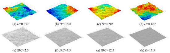
Figure 1.
The interpolation function diagram and schematic diagram of the fracture surface. (a–d) are the interpolation function diagrams corresponding to different fractal dimensions. (e–h) are the schematic diagrams of fracture surface with JRC values determined by the fractal dimensions.
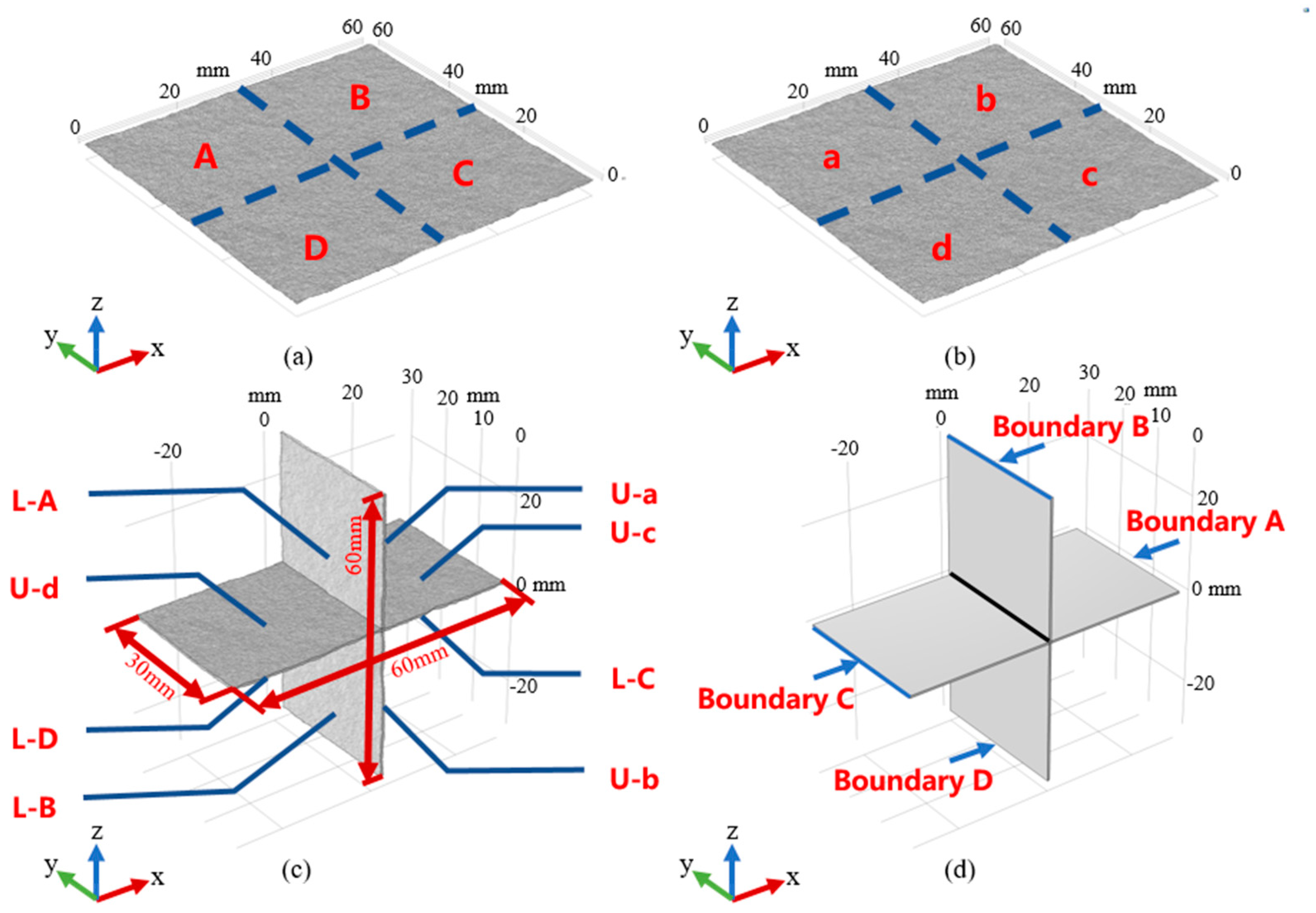
Conventionally, the two surfaces of the fracture are matched, so a fracture can be represented by two same surfaces that are separated by a small distance. The dimensions of the fracture surfaces generated by COMSOL were all 60 mm × 60 mm, and the upper surface was obtained by raising the lower fracture surface by 0.5 mm; Then the upper surface was misaligned by 1 mm along the x-axis to investigate the shear effect. In Figure 2, the upper and lower surfaces of the fracture model were labeled as U and L, respectively. Both surfaces were symmetrically divided into four areas to define the four branches of the fracture intersection.
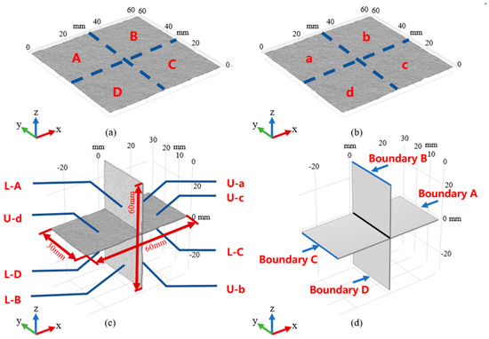
Figure 2.
Upper and lower fracture surface area division, crossed fracture model, and illustration of the fracture walls. (a) Upper surface; (b) lower surface; (c) crossed rough-walled fracture model; and (d) illustration of the fracture walls. The top, bottom, left, and right walls (in blue) were termed as boundaries A, B, C, and D, corresponding to branches 1, 2, 3, and 4, respectively.
The fracture surfaces with JRC values of 2.5, 7.5, 12.5, and 17.5 were operated to generate crossed fracture models with different roughness, and the fracture models with a JRC of 17.5 are presented in Figure 2. It shows that the 3D crossed fracture model was 60 mm in the X-direction, 30 mm in the Y-direction, and 60 mm in the Z-direction; the horizontal and vertical fracture surfaces intersected at right angles, and their different surface morphology was different in each these branches, which was beneficial and convenient for studying the evolution of fluid flow and solute transport in terms of the change of fracture surface roughness properties. The division of each area of the upper and lower fracture surfaces is presented in Figure 2a,b. The 3D crossed fracture model is presented in Figure 2c, and the top, bottom, left, and right walls (in blue) were termed as boundaries A, B, C, and D, which corresponded to branches 1, 2, 3, and 4 (Figure 2d).
Fracture surfaces with JRC values of 2.5, 7.5, 12.5, and 17.5 were used to generate crossed fracture models with varying roughness. Figure 2 illustrates the model with a JRC of 17.5. The 3D crossed fracture model dimensions were 60 mm 60 in the X-direction, 30 mm in the Y-direction, and 60 mm in the Z-direction. The horizontal and vertical fracture surfaces intersected at right angles, and the varying surface morphologies across the branches facilitated the study of fluid flow and solute transport evolution with changes in fracture surface roughness properties. The division of the upper and lower fracture surfaces into distinct areas is shown in Figure 2a,b. The 3D crossed fracture model is depicted in Figure 2c. The top, bottom, left, and right walls, highlighted in blue, were labeled as boundaries A, B, C, and D, corresponding to branches 1, 2, 3, and 4, respectively, as shown in Figure 2d.
2.2. Fracture Surface Roughness Characteristic
To analyze variations in local aperture, the four sets of crossed fracture intersections were divided into 30 equidistant sections along the Y-axis, resulting in 31 profiles (Figure 3). The edge lengths of the profiles corresponding to branches 1, 2, 3, and 4 were measured in COMSOL and considered as the local aperture for each respective branch. The location of the intersection region (HT) of the crossed fractures is shown in Figure 3a, while the positions of the 31 equidistant profiles are illustrated in Figure 3b.

Figure 3.
(a) HT position of the crossed fractures intersection part; (b) geometric structure of the intersection part and division of the local aperture measurement profile.
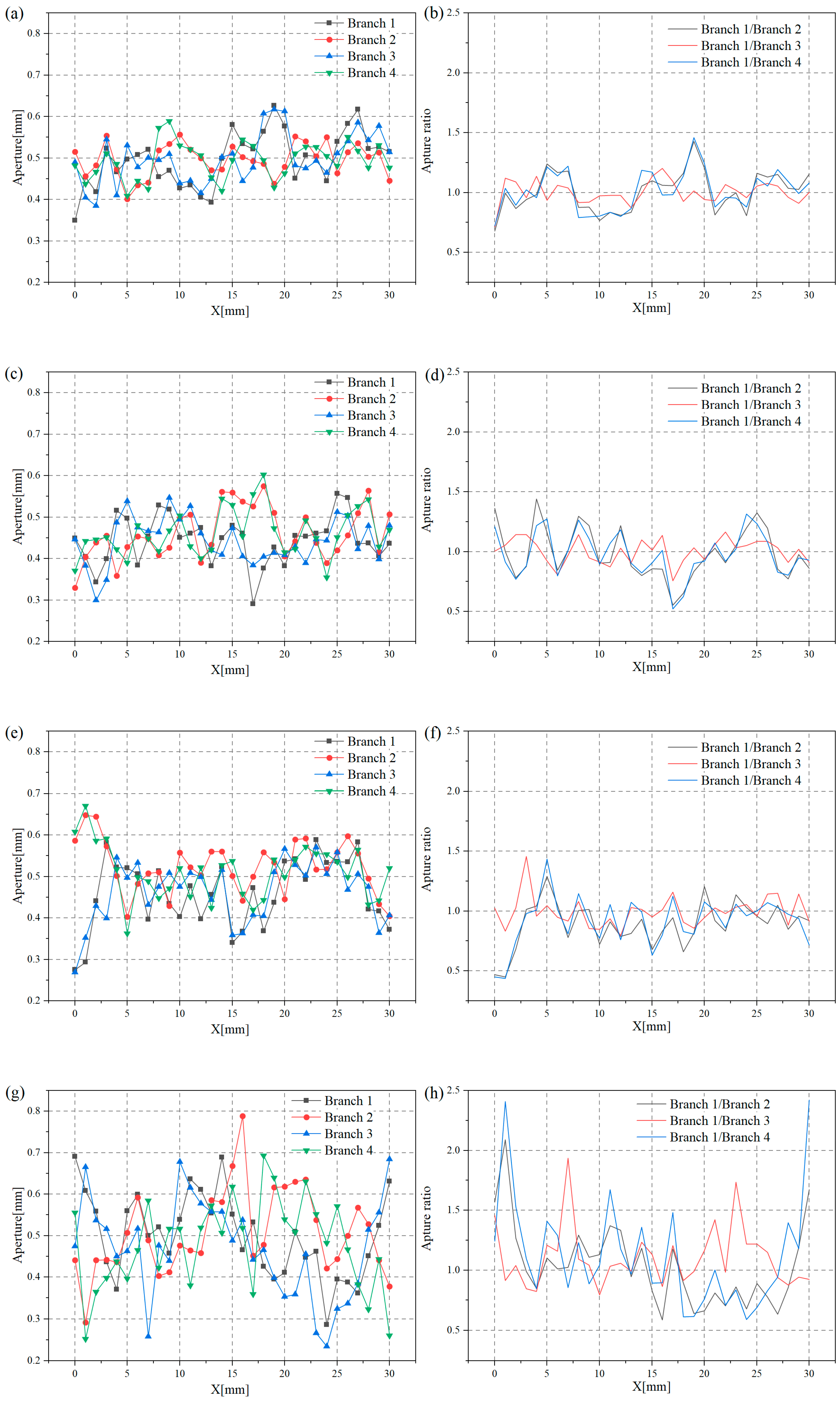
To characterize the geometric features of the intersection, Figure 4a,c,e,g show the local aperture variations of the four branches along the Y-axis, while Figure 4b,d,f,h illustrate the local aperture ratios of branch 1 to branches 2, 3, and 4, respectively. The variation of the local aperture along the Y-axis across the four branches demonstrates significant fluctuation around the average aperture of 0.5 mm, indicating a high degree of irregularity in the intersection’s geometric structure. For example, when JRC = 17.5, the local aperture ratios revealed the following trends:
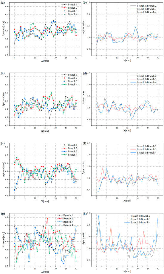
Figure 4.
Local aperture at the intersection of the four branches along the Y-axis and local aperture ratios between branch 1 and branch 2, between branch 1 and branch 3, and between branch 1 and branch 4. (a,c,e,g) correspond to the local apertures when JRC values were 2.5, 7.5, 12.5, 17.5, respectively, and (b,d,f,h) are the respective local aperture ratios.
(1) Branch 1 vs. branch 2: the local aperture of branch 1 was generally larger than that of branch 2 in the Y-coordinate ranges of 1–3 mm, 7–15 mm, and 28–30 mm, while branch 2 exhibited a slightly smaller aperture in the ranges of 3–7 mm and 15–28 mm.
(2) Branch 1 vs. branch 3: branch 1 and branch 3 displayed similar local apertures, except in specific areas (Y-coordinate ranges of 5–9 mm and 19–27 mm), where branch 1 had a larger aperture.
(3) Branch 1 vs. branch 4: the local aperture of branch 1 was generally larger than that of branch 4 in the Y-coordinate ranges of 0–5 mm, 10–17 mm, and 27–30 mm, while branch 4 had a slightly smaller aperture in the ranges of 5–10 mm and 14–27 mm.
The study investigated crossed fracture models with surface roughness values of 2.5, 7.5, 12.5, and 17.5, and similar trends were observed for the other roughness conditions. From Figure 4a,c,e,g, it is evident that the amplitude of local aperture fluctuations increased with higher JRC values, suggesting that the irregularity of the intersection geometry became more pronounced as surface roughness increased.
Figure 4b,d,f,h further indicate that the local aperture ratio divergence and variability between branches also increased with higher JRC values. This highlighted that the intensity of local aperture variation in crossed fractures was dependent on the magnitude of surface roughness. Additionally, the locations of abrupt changes in the local aperture can serve as a reference for predicting the distribution of flow streamlines and solute transport concentration fields.
3. Crossed Fracture Seepage and Solute Transport Numerical Modeling
3.1. Method and Governing Equation for Fluid Flow and Solute Transport
3.1.1. Material and Method
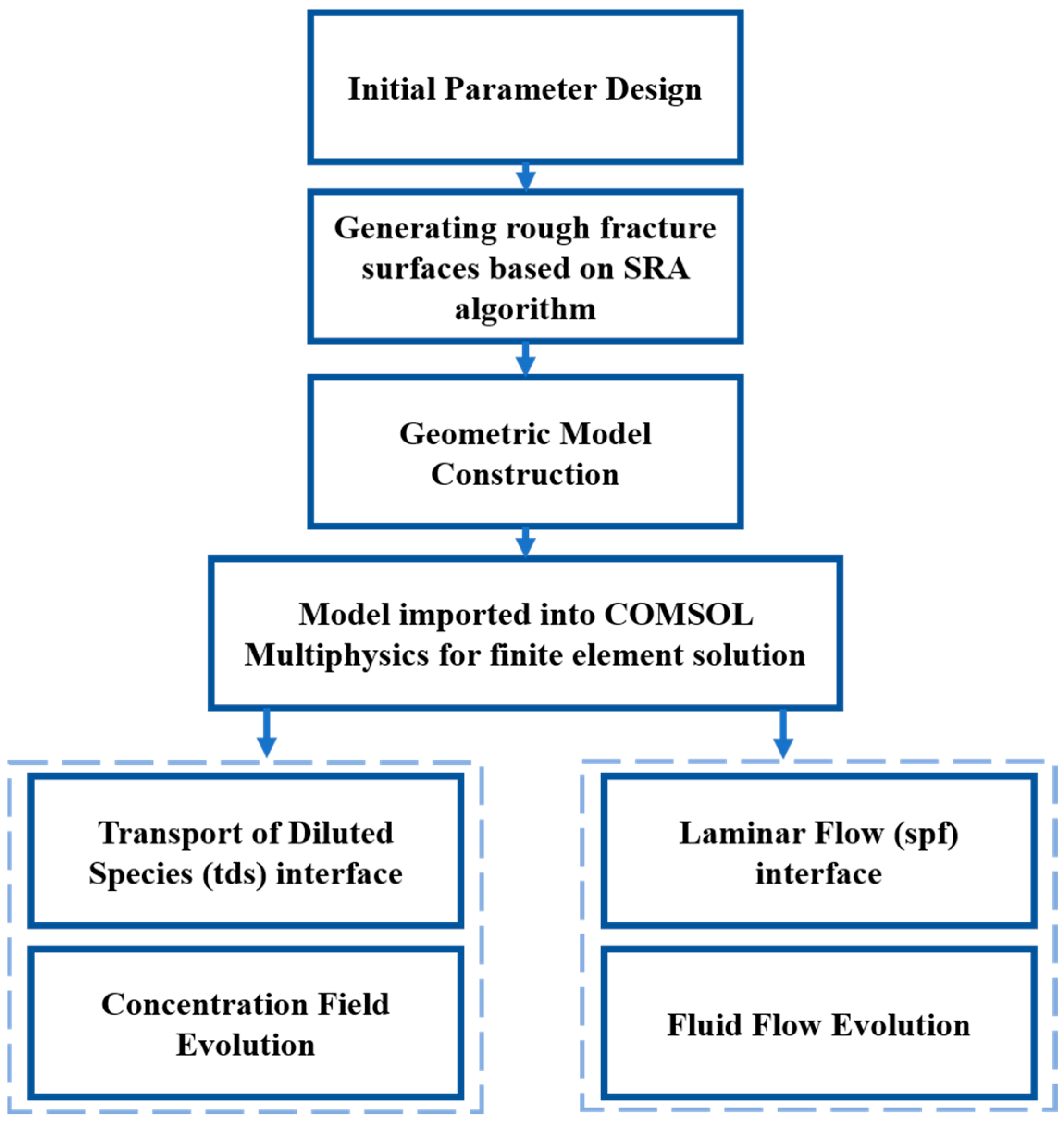
The crossed fracture model in this study ignores material effects and considers only the processes by which the geometry affects fluid flow and solute transport. Compared with other numerical simulation software, COMSOL Multiphysics 6.2 can provide abundant physical field modules. These modules lay the foundation for establishing numerical models of cross-fracture fluid flow and solute transport in COMSOL and solving the coupled nonlinear equation system efficiently [41]. Following the modeling of the crossed fracture in COMSOL Multiphysics, the Laminar Flow and Transport of Diluted Species interfaces were utilized for the coupled analysis. The Laminar Flow interface sets the fluid as an incompressible flow, and the Transport of Diluted Species interface set the additional transport mechanism to convection. The algorithm and COMSOL interface used for numerical simulation are shown below (Figure 5).
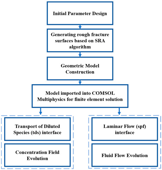
Figure 5.
Method block diagram.
3.1.2. Governing Equations for Fluid Flow
Since fractures are non-homogeneous, the fracture unit takes the form of a parallel plate while incorporating information on the spatial aperture variation of the fracture [42,43]. For incompressible Newtonian fluids with constant viscosity coefficients, which maintain steady-regime flow in rough fractures, they can be accurately described by the Navier−Stokes equations (NSEs) representing momentum and mass conservation, and their governing equations can be expressed as:
where ρ (kg/m3) is the fluid density, u (m/s) is the fluid velocity, p (Pa), and μ (Pa·s) is the fluid dynamic viscosity.
3.1.3. Governing Equations for Solute Transport
Bodin et al. [44,45] investigated the physical mechanisms of solute transport in fractured rock masses, which primarily include convection, dispersion, and diffusion. In this study, we focus on the solute transport characteristics of crossed fractures, considering only two physical mechanisms: convection and diffusion. The steady-state solute transport is generally governed by the advection-diffusion equation, which describes the solute transport process in crossed fractures over time. This equation can be expressed as:
where C (kg/m3) is the solute concentration, t is the time, and D (m2/s) is the molecular diffusion coefficient.
3.2. Boundary and Initial Condition
3.2.1. Boundary Condition
In this paper, the study was carried out at the fractures without considering the flow and transport processes within the rock matrices, so all fracture surfaces and contact boundaries were considered impermeable and slip-resistant. The flow rate was used to represent the inlet boundary of the flow in the fracture, and the flow could enter the rock fracture freely according to the local aperture of the inlet surface, which could effectively reduce the boundary effect. Each branch fracture surface of crossed fractures was set as sealed anti-slip walls (u = 0), and the pressure at the flow outlet boundary was set as zero pressure (p = 0). In order to facilitate the control of the Péclet number and the calculation of the mixing ratio, the inlet flow boundary of the two inflow branches was set to have an equal flow rate (Q1 = Q2 = Q3). In the initial regime, there was no solute in the fracture void (C = 0), and from time t = 0, the solute started to flow into the boundary and kept the concentration C = C0 constant. All the other boundaries were set as no-flux.
In this study, the analysis was conducted on fractures without considering flow and transport processes within the surrounding rock matrix. Consequently, all fracture surfaces and contact boundaries were assumed to be impermeable and slip-resistant. The flow rate was used to define the inlet boundary conditions for flow within the fracture. The flow could freely enter the rock fracture based on the local aperture of the inlet surface, effectively minimizing boundary effects. Each branch fracture surface of the crossed fractures was modeled as sealed, anti-slip walls (u = 0), while the outlet boundary was set to zero pressure (p = 0). To facilitate the control of the Péclet number and the calculation of the mixing ratio, the inlet flow boundaries of the two inflow branches were assigned equal flow rates (Q1 = Q2 = Q3). At the initial state (t = 0), the fracture void was free of solutes (C = 0). From t = 0 onward, solute began to enter the boundary with a constant concentration (C = C0). All other boundaries were set to no-flux conditions.
The Navier−Stokes equations (NSEs) and the transport equation formed a set of nonlinear partial differential equations that coupled velocity, pressure, and concentration fields. In this study, the commercial finite element software COMSOL Multiphysics 5.6 was used to sequentially solve the NSE and transport equations. The steady-state flow and solute transport for each solution were computed over 10 times the average residence time, requiring approximately 18 h on a high-performance workstation.
3.2.2. Initial Condition
The characteristic parameters of the fluid in the simulation and adopted boundary conditions are summarized in Table 1. In order to characterize the effects of surface roughness and fracture intersections on flow transport processes in crossed fractures under different flow conditions, six inlet flow conditions with different flowrates were selected in this study, from which six different sets of the Reynolds number and the Péclet number were obtained. The Re and Pe are defined as:
where (m/s) is the mean fluid inflow velocity, (m) is the characteristic length approximated by the mean fracture aperture, Q (m3/s) is the inlet flowrate, and W (m) is width of fracture. The Re and Pe selected in this study belonged to a one-to-one correspondence, and the range of values usually existed under natural flow conditions.

Table 1.
Characteristic parameters of the fluid in the simulation and adopted boundary conditions.
For fluid flow properties, water with a constant density of = 9.997 × 10² kg/m3 and a dynamic viscosity of = 1.307 × 10⁻³ Pa·s was used as the fluid. To ensure laminar flow throughout the study, the Reynolds number (Re) was maintained below 1, which corresponded to a Péclet number (Pe) of less than 600. Various flow rates (Q) were applied at the inlet boundary, resulting in Péclet numbers ranging from 0.1 to 600. This range is considered to be within the linear laminar flow regime with negligible turbulence effects.
To investigate the solute transport properties at the fracture intersection, a constant solute concentration C0 was injected at the boundary A to perform transport simulations. In order to eliminate the effect of the magnitude between the results and to facilitate the comparison of the results, a normalization process was performed to normalize the concentration to . Unless specified otherwise, the results reported in the following sections used the normalized time , where is the average residence time for fluid flow through the fracture (, where L is the length of fracture and u is the averaged flow velocity in the fracture in the principal direction of each branch).
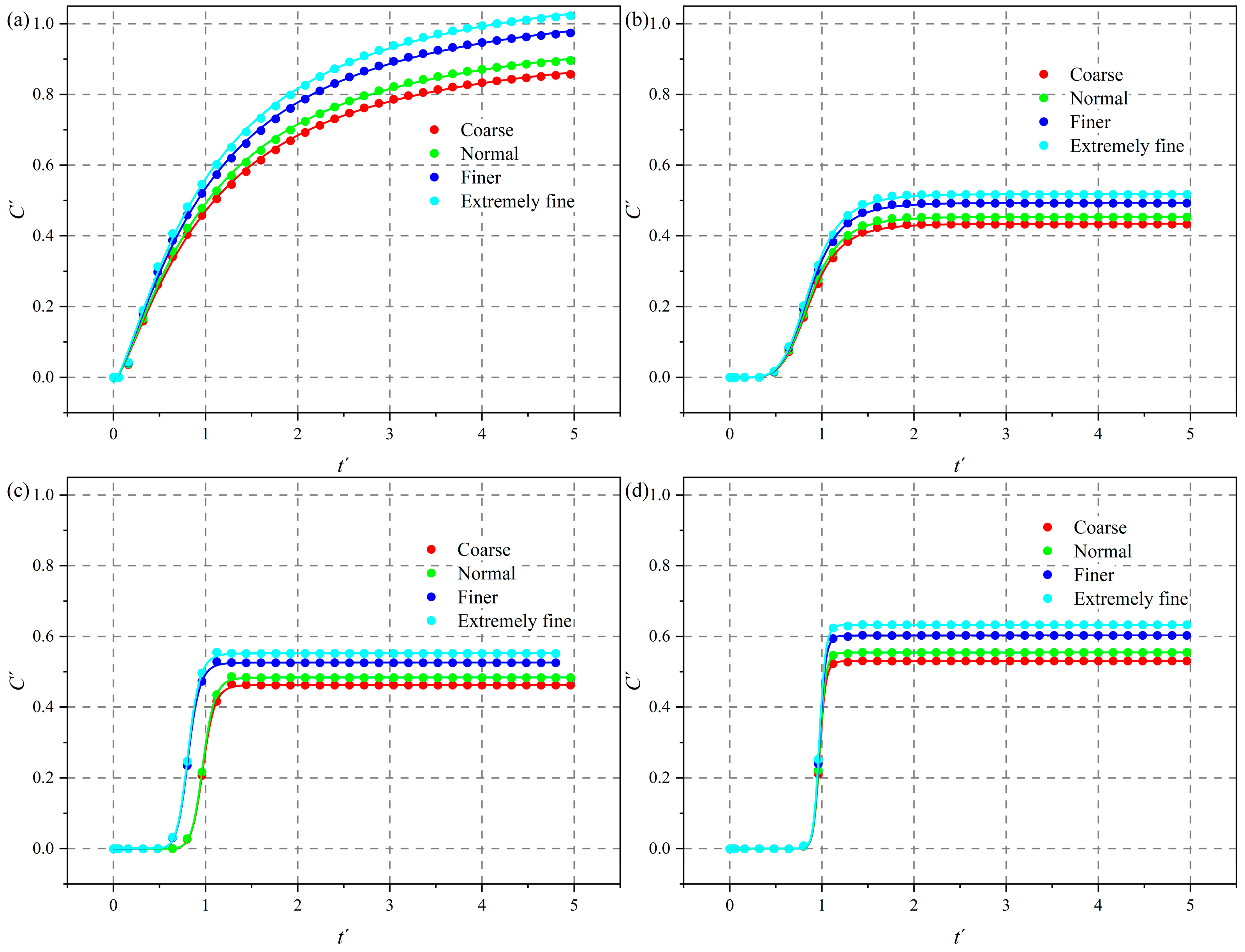
3.2.3. Mesh Independence Check
To ensure the accuracy of the crossed fracture model, it is essential to verify that the mesh size does not influence the calculation results. Fluid flow simulations were performed on four crossed fractures using four different mesh settings: coarse, normal, finer, and extremely finer. Figure 6 illustrates the effects of these mesh settings on the mean solute concentration at the outflow boundary B. The results indicated that the mean solute concentration varied noticeably across the four mesh settings. Specifically, the concentrations obtained with coarse and normal meshes were significantly lower than those obtained with finer and extremely finer meshes. However, the difference in mean solute concentration between the finer and extremely finer settings was negligible, suggesting that further refinement of the mesh had minimal impact on the results at this resolution. Therefore, to balance computational efficiency and accuracy, the finer mesh setting was adopted for this study.
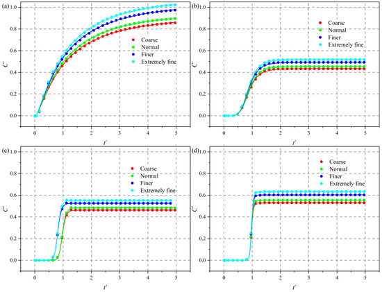
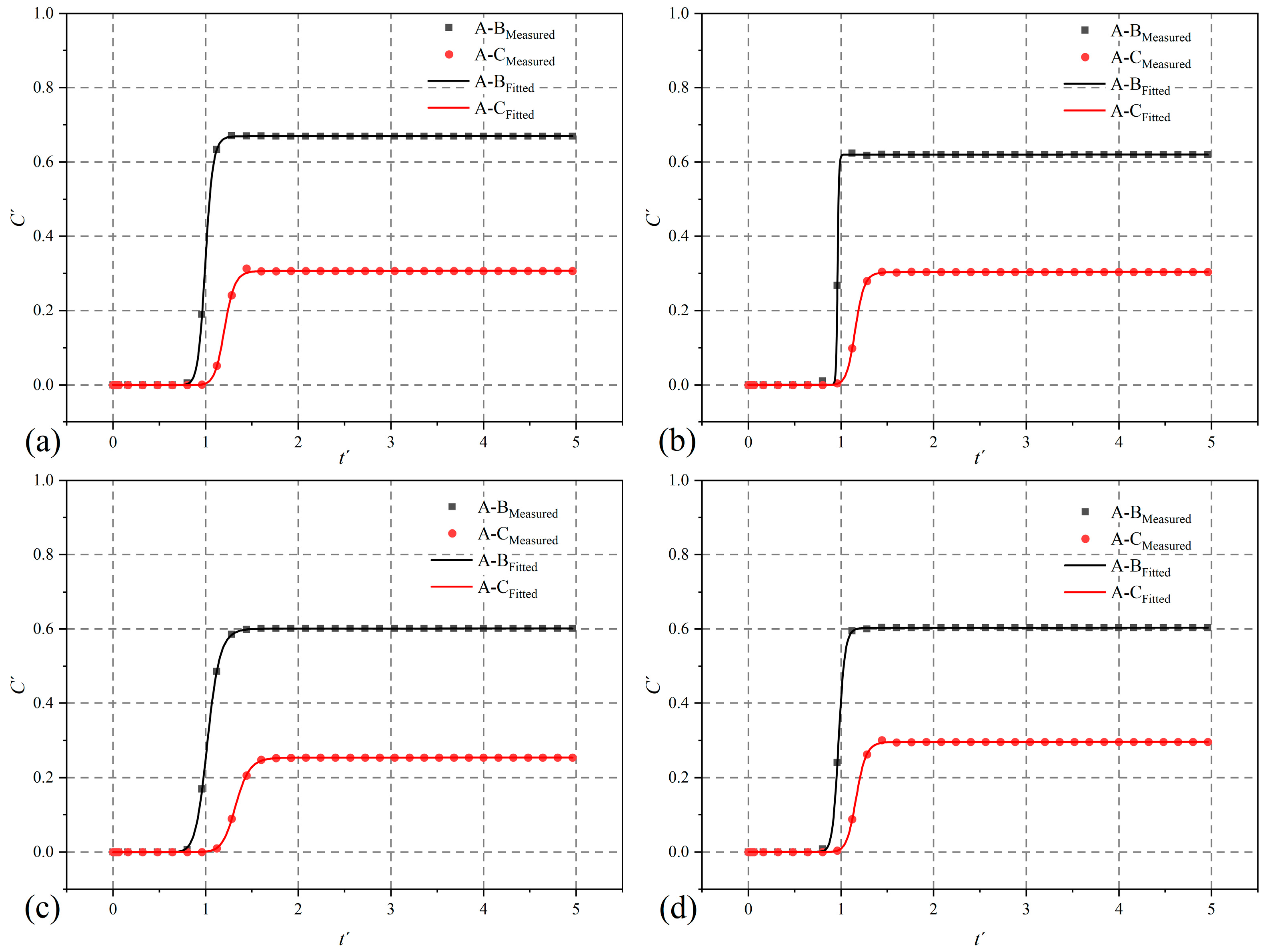
Figure 6.
Breakthrough curves at boundary B with different mesh settings when JRC = 17.5: (a) Pe = 1; (b) Pe = 10; (c) Pe = 100; (d) Pe = 600.
4. Results and Discussions
4.1. Channeling Flow Variations in the Flow Field
The flow field in crossed fractures was first examined, as it serves as the foundation for studying the subsequent solute transport process. In particular, channeling flow within the flow field significantly impacts the solute transport process. Two primary factors that enhance channeling flow at fracture intersections are flow rate and surface roughness. These factors influence the flow field and solute transport differently, necessitating an independent investigation of their effects for accurate quantitative characterization.
4.1.1. Effect of Pe
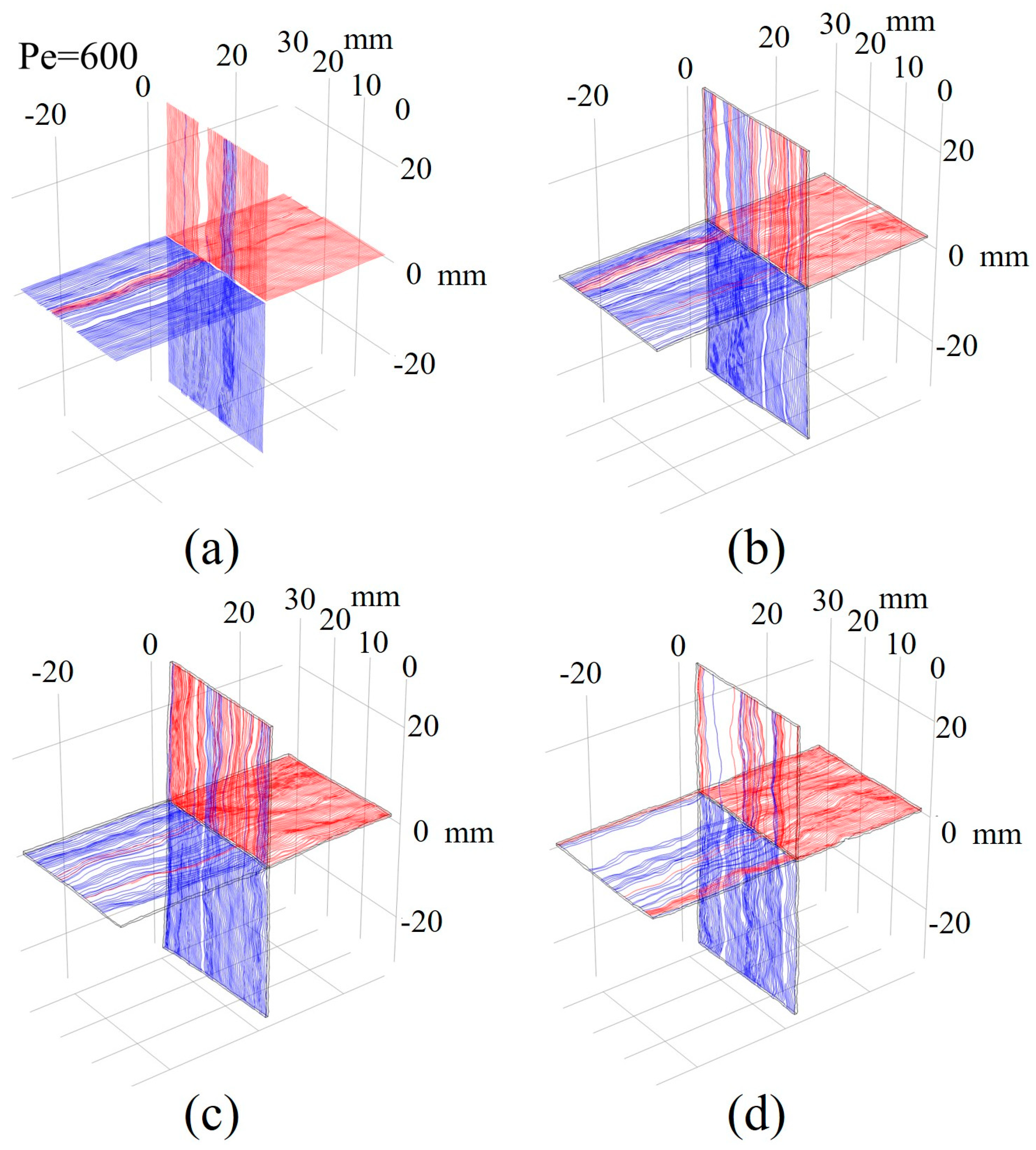
To investigate the flow field variation under the influence of Pe, a series of fluid flow models with fixed surface roughness and changing Pe were set up to investigate the variation of the flow field. Figure 7 presents flow streamlines in four crossed fractures for JRC = 17.5, as the typical result of the inlet/outlet pattern at the intersection. Since two outlets had the same flow rate (Q1 = Q2) and the same average apertures of the two fractures, the flow rates at the two outlets were nearly the same. In order to highlight the flow redistribution at the intersection, the flows from different outlets were differentiated by different colors, i.e., red and blue for inflow branches 1 and 4, respectively.
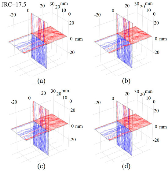
Figure 7.
Evolution of the flow fields for JRC = 17.5 with increasing Pe: (a) Pe = 1; (b) Pe = 10; (c) Pe = 100; (d) Pe = 600.
To study the variation of the flow field under the influence of the Péclet number (Pe), a series of fluid flow models were constructed with fixed surface roughness and varying (Pe) values. Figure 7 illustrates the flow streamlines in four crossed fractures (JRC = 17.5), representing a typical inlet/outlet pattern at the intersection. Since the two outlets had identical flow rates (Q1 = Q2) and the average apertures of the two fractures were the same, the flow rates at the two outlets were nearly equal. To emphasize the flow redistribution at the intersection, the flows from different outlets are distinguished by colors: red and blue, representing inflow branches 1 and 4, respectively.
The continuous flow streamlines from branches 1 to 3 and branches 4 to 2 clearly demonstrated channeling flow behavior at the intersection. In all four figures, a few red streamlines originating from inflow branch 1 were diverted into outflow branch 3, while a similar number of blue streamlines from inflow branch 4 were diverted into outflow branch 2. The channeling flow at the fracture intersection became increasingly pronounced as Pe increases. For Pe = 1 (Figure 7a), the channeling flow was limited to a small area. As Pe rose (Figure 7b–d), the number of channeling flow streamlines increased, and the area affected by channeling flow expanded correspondingly.
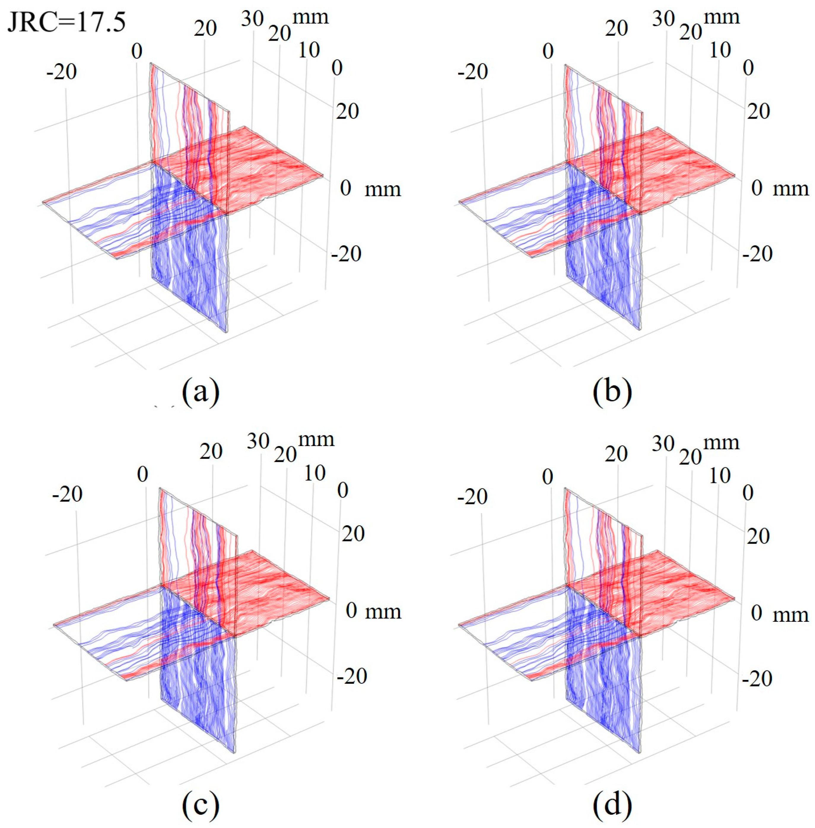
4.1.2. Effect of JRC
Same as the research method in Section 4.1.1, a series of fluid flow models with fixed Pe and changing JRC were set up to investigate the variation of the flow field. Figure 8a–d present that with the increasing JRC, the curvature of the streamlines increased and the occurrence of channeling flow was more frequent. In particular, to investigate the area where channeling flow occurred, the flow field when JRC = 17.5 was analyzed (Figure 8d). The channeling flow from the branch 1 into branch 3 occurred in the ranges of Y = [0, 5 mm], [10 mm, 17 mm], and [27 mm, 30 mm], where the local aperture of branch 1 was larger than that of branch 4 (Figure 4h). In the same way, the channeling flow from the branch 4 into branch 2 occurred in the ranges of Y = [5 mm, 10 mm] and [17 mm, 27 mm], where the local aperture of branch 4 was larger than that of branch 1 (Figure 4h). Comparing the local aperture ratio (Figure 4h) with the flow field (Figure 8d) showed that channeling flow tended to occur at the location where the local aperture expanded sharply. In summary, surface roughness affected the fracture geometry and the local aperture variation at the intersection, which affected the curvature of the flow streamlines and the distribution of channeling flow.
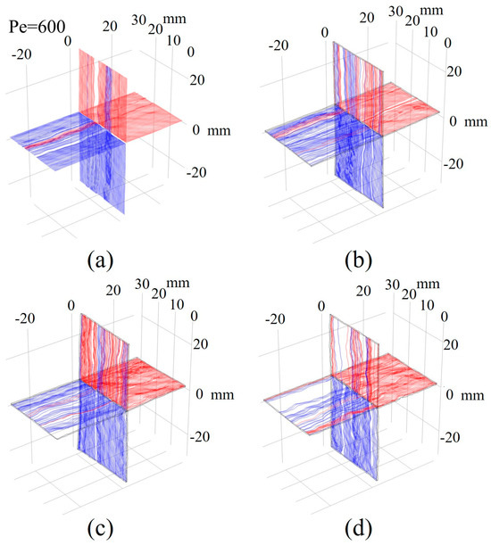
Figure 8.
The evolution of the flow fields with increasing Pe for different JRC values: (a) JRC = 2.5; (b) JRC =7.5; (c) JRC =12.5; (d) JRC =12.5. In addition, the aperture variation zones are marked when JRC = 17.5.
Using the same research method as described in Section 4.1.1, a series of fluid flow models with fixed (Pe) and varying (JRC) values were established to investigate the variation in the flow field. Figure 8a–d demonstrate that as JRC increased, the curvature of the streamlines became more pronounced, and the frequency of channeling flow occurrence rose. To analyze the areas where channeling flow occurred, the flow field for JRC = 17.5 was examined (Figure 8d). The channeling flow from branch 1 into branch 3 occurred in the Y-coordinate ranges of [0–5 mm], [10–17 mm], and [27–30 mm], where the local aperture of branch 1 was larger than that of branch 4 (as shown in Figure 4h). Similarly, the channeling flow from branch 4 into branch 2 occurred in the ranges of [5–10 mm] and [17–27 mm], where the local aperture of branch 4 exceeded that of branch 1 (Figure 4h). Comparing the local aperture ratio (Figure 4h) with the flow field (Figure 8d) revealed that channeling flow was more likely to occur in locations where the local aperture expanded sharply. In summary, surface roughness influenced the fracture geometry and the variation in local aperture at the intersection, which, in turn, affected the curvature of the flow streamlines and the spatial distribution of channeling flow.
In addition, it is known from previous studies that the fluid flow in the parallel-plate model always follows the streamline pattern and no channeling flow occurs with the change of Pe.
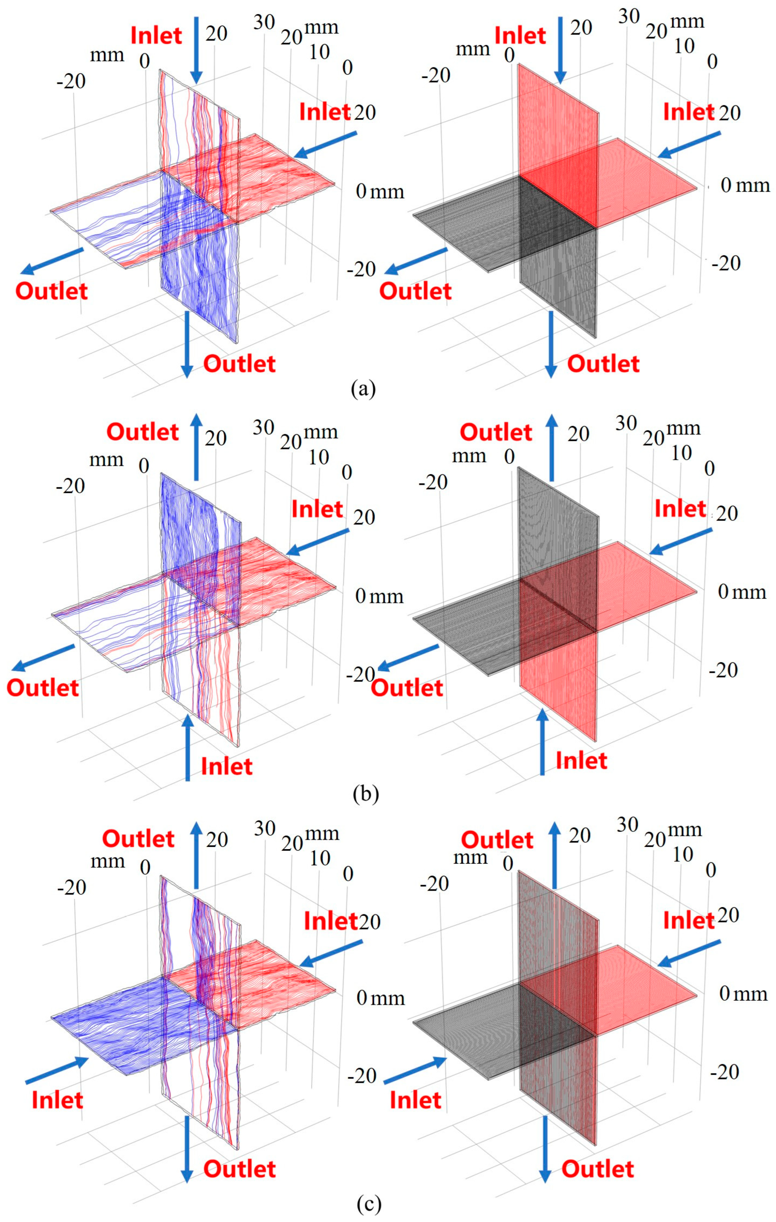
To examine the effect of surface roughness anisotropy on channeling flow, the flow fields under three different inlet/outlet combinations were analyzed. For JRC = 17.5 and Pe = 600, the flow fields of rough-walled and parallel-plate crossed fracture models under these combinations are presented in Figure 9. Figure 9 shows that the flow field in parallel-plate crossed fractures was uniform and symmetric. Fluid entered from one boundary and exited through another without significant interaction at the intersection. In contrast, in the rough-walled model, the anisotropic surface roughness altered the flow streamline distribution, leading to channeling effects at the intersection. Additionally, due to the relatively small scale of the crossed fracture model, the effect of gravity on the distribution of flow streamlines could be considered negligible.
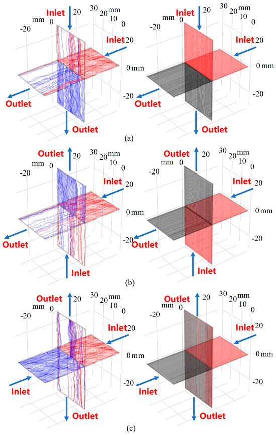
Figure 9.
Comparison of flow fields between rough-walled and parallel-plate crossed fracture models. (a) Comparison of flow field distribution of combination 1 (inlets 1 and 4); (b) comparison of flow field distribution of combination 2 (inlets 1 and 2); and (c) comparison of flow field distribution of combination 3 (inlets 1 and 3).
Figure 9 further illustrates that the flow field in rough-walled crossed fractures resulted in significant channeling flow, with distinct streamline patterns for different inlet/outlet combinations. The curvature of the streamlines was attributed to the non-homogeneity of the cavity in rough-walled fractures, and the occurrence of channeling flow was closely linked to variations in the local aperture. For combination 1, the pattern of channeling flow occurrence has been previously discussed. Following the same analysis for combination 2, the channeling flow from branch 1 into branch 3 occurred within the Y-coordinate ranges of [1–3 mm], [7–15 mm], and [28–30 mm], where the local aperture of branch 1 was larger than that of branch 2 (Figure 4h). Similarly, the channeling flow from branch 2 into branch 4 occurred within the ranges of [3–7 mm] and [15–28 mm], where the local aperture of branch 2 exceeded that of branch 1 (Figure 4h). For combination 3, branches 1 and 3 had similar local apertures, resulting in a more random occurrence of channeling flow. In summary, the patterns of channeling flow across different combinations reinforced the conclusion that local aperture variations determined the areas where channeling flow occurred. Additionally, the anisotropy of surface roughness played a critical role in shaping the curvature of flow streamlines, further emphasizing its influence on flow behavior in rough-walled crossed fractures.
4.2. Evolution of Concentration Fields
4.2.1. Effect of Pe
Figure 10 illustrates the evolution of the concentration field of the crossed fracture models at different times . Taking JRC = 17.5 and Pe = 0.1, 1, 10, 100, 300, and 600 as examples, significant differences in concentration distribution characteristics under varying flow conditions were analyzed. In this study, combination 1 was selected as the inlet/outlet configuration for fluid flow. Solute entered the fracture system through boundary A with a constant concentration of 1 kg/m3, providing a clear basis for evaluating solute transport and mixing behavior under different flow regimes.
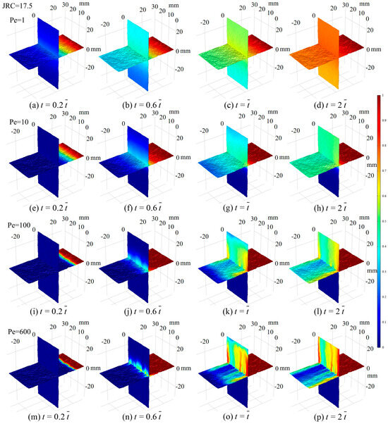
Figure 10.
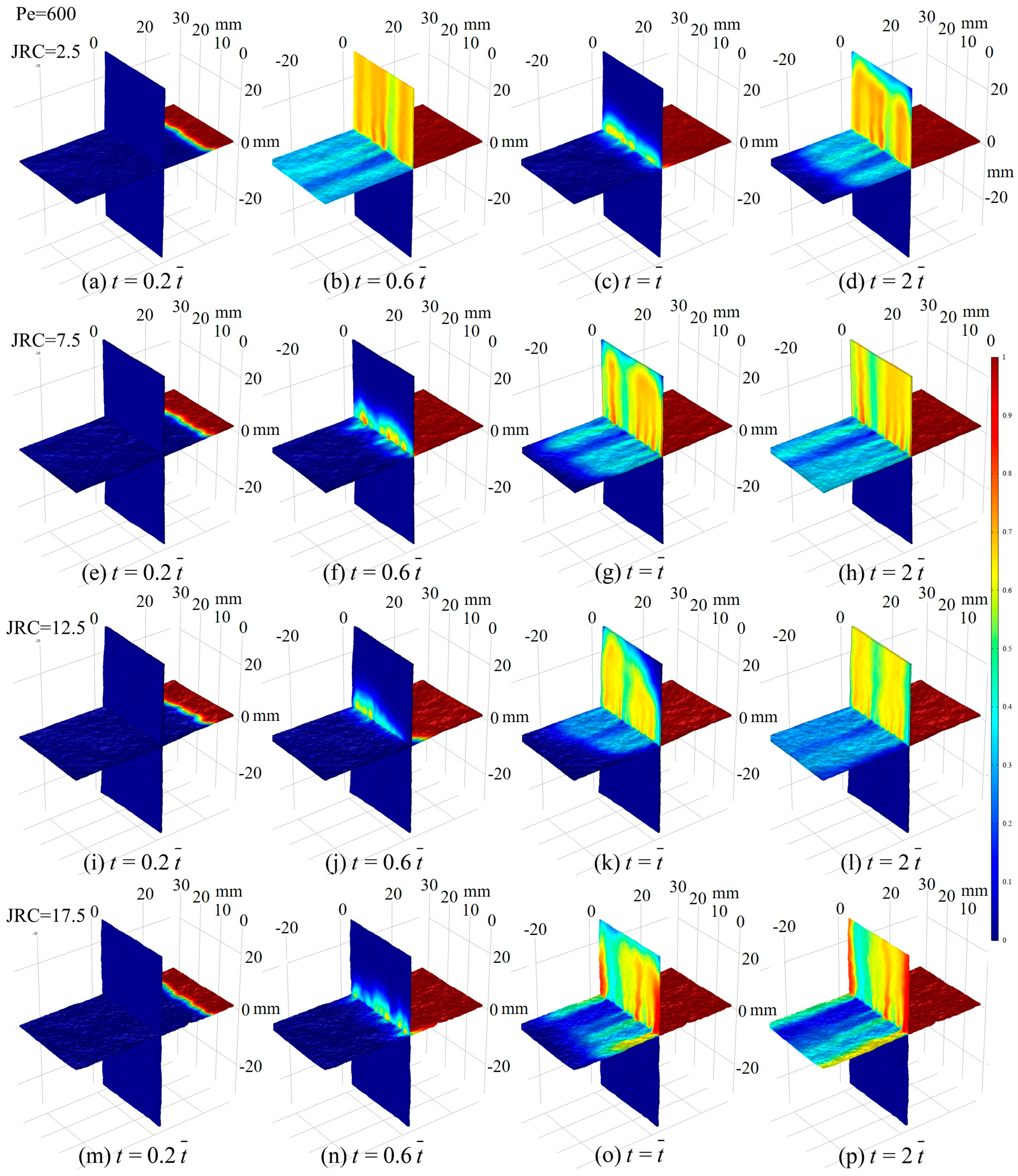
Evolution of the concentration distributions for different Pe when JRC = 17.5: (a–d) Pe = 1; (e–h) Pe = 10; (i–l) Pe = 100; (m–p) Pe = 600.
For Pe = 1 (Figure 10a–d), the concentration field was basically homogeneously spreading along branch 1 to branches 2, 3, and 4, since the molecular diffusion played a dominant role in solute transport for small values of Pe (i.e., Pe < 10). From to (Figure 10a,b), the solute mixed at the intersection of the fracture and then continued to spread to the three outlets, and the concentration variation along the transport direction was nearly zero. It can be shown that the fluid flow had less effect on solute transport and molecular diffusion of solutes played a dominant role when Pe < 10.
For Pe = 10 (Figure 10e–h), the concentration field maintained homogeneously spreading along the branch 1 to branches 2 and 3, since the complete mixing mode of fluid transport mode played a dominant role in solute transport for 10 < Pe < 100. From to (Figure 10f–h), the solute mixed at the intersection and then continued to spread to the two outlets, and the concentration variation along the transport direction was nearly zero. Previous studies have shown that ideal fluid transport modes include complete mixing mode. The solute was well mixed at the intersection and then diffused to outflow branches 2 and 3. Diffusion of the solute still played a dominant role at this point, but it no longer diffused into the inflow branch 4. It can be shown that the fluid flow began to have an effect on solute transport and the complete mixing mode played a dominant role when 10 < Pe < 100.
For Pe = 100 (Figure 10i–l), the concentration field gradually showed a higher concentration in branch 2 than in branch 3, indicating that mixing of solutes at the intersection decreased with increasing Pe. From to (Figure 10j–l), the solute mixed at the intersection and then continued to spread to the two outlets, and the concentration was higher along the streamline path. Previous studies have shown that ideal fluid transport modes include the streamline routing mode. For Pe > 100, convection began to dominate solute transport, with a significant increase in the proportion of solutes transported along the streamline.
For Pe = 600 (Figure 10m–p), the concentration fields in branches 2 and 3 showed strong channelization along the streamline path, indicating that the effect of the local aperture on the concentration distribution began to emerge with increasing Pe. Same as Pe = 100, the solute transport process followed the streamline routing mode. As Pe increased, the concentration difference between outflow branches 2 and 3 first widened and then tended to be constant, and the channelization of the concentration field became more pronounced.
Comparing the concentration field distributions under different Pe, it is evident that molecular diffusion dominated when Pe < 10. As Pe increased, the streamline path mode gradually became the dominant transport mechanism. In summary, solute transport under varying Pe was controlled by different factors, leading to distinct evolution patterns in the concentration field. This further highlight that the solute transport process is strongly dependent on the flow rate.
4.2.2. Effect of JRC
Figure 11 presents the evolution of the concentration field of crossed fractures at different times 0.2, 0.6, 1.0, and 2.0. Taking Pe = 600, JRC = 2.5, 7.5, 12.5, and 17.5 as an example, the significant differences in the concentration distribution characteristics for different flow conditions were analyzed.

Figure 11.
Evolution of the concentration distributions for different JRC values when Pe = 600: (a–d) JRC = 2.5; (e–h) JRC = 7.5; (i–l) JRC = 12.5; (m–p) JRC = 17.5.
For (Figure 11a,e,i,m), the evolutions of the concentration field were approximately the same for JRC = 2.5, 7.5, 12.5, and 17.5. As (Figure 11b,f,j,n), the concentration fields evolved to the fracture intersection and the distribution of the concentration field started to diverge. For t = 1.0 and t = 2.0, the concentration fields in branches 2 and 3 showed strong channelization along the streamline path, indicating that the effect of the local aperture on the concentration distribution began to emerge as time went by.
For JRC = 2.5, the channelization of the concentration field in branch 2 occurred in the ranges of Y= [4 mm, 7 mm], [13 mm, 21 mm], and [25 mm, 30 mm], where the local aperture of branch 1 was larger than that of branch 4 (Figure 4b).
For JRC = 7.5, the channelization of the concentration field in branch 2 occurred in the ranges of Y= [0, 1 mm], [3 mm, 5 mm], [7 mm, 12 mm], and [23 mm, 27 mm], where the local aperture of branch 1 was larger than that of branch 4 (Figure 4d).
For JRC = 12.5, the concentration field was uniform in branch 2, where the local apertures of branch 1 and branch 4 were nearly the same (Figure 4f).
For JRC = 17.5, the channelization of the concentration field in branch 2 occurred in the ranges of Y= [0, 5 mm], [10 mm, 17 mm], and [27 mm, 30 mm], where the local aperture of branch 1 was larger than that of branch 4 (Figure 4h).
According to the above analysis of the local aperture under different JRC values, the evolution of the concentration field presented that the concentration-enriched areas of branch 3 were all located at the drastic change of the local aperture. In addition, as JRC increased, the curvature of the concentration field distribution was enhanced. In summary, surface roughness affected the solute concentration field distribution by influencing the local aperture at the intersection.
Based on the above analysis of local aperture variations under different JRC values, the evolution of the concentration field indicated that the concentration-enriched areas in branch 3 consistently corresponded to regions with drastic changes in local aperture. Additionally, as JRC increased, the curvature of the concentration field distribution became more pronounced. In summary, surface roughness significantly influenced the solute concentration field distribution by affecting the local aperture variations at the fracture intersection.
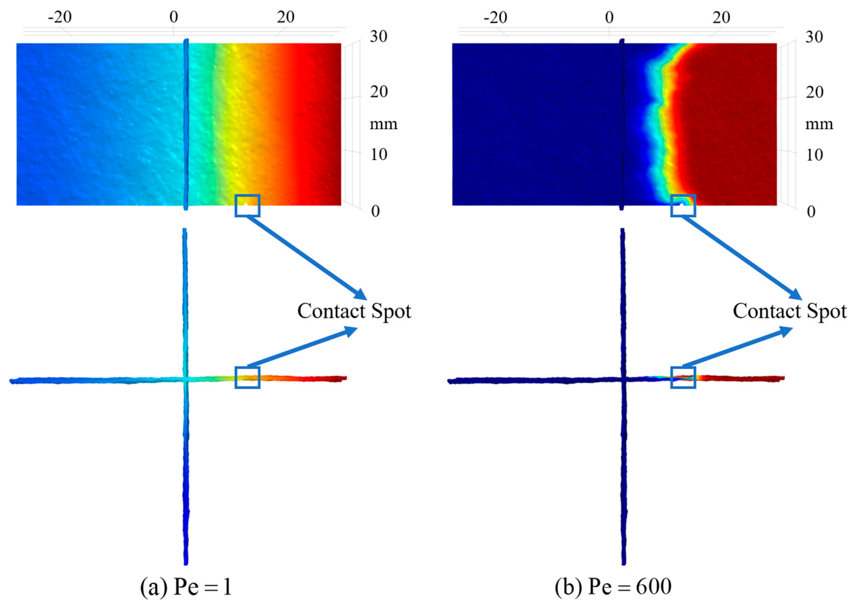
Figure 12 illustrates the evolutions of the concentration field in the XY plane and the Y = 0 cross-section for different Pe values when . The cases of Pe = 1 and Pe = 600 were highlighted to exemplify the significant differences in concentration distribution characteristics under low- and high-flow-rate conditions. These comparisons revealed distinct transport behaviors influenced by the flow conditions.

Figure 12.
Concentration evolutions in the XY plane direction and in the Y = 0 cross-section for different Pe when : (a) Pe = 1; (b) Pe = 600.
In the low-flow-rate case, when Pe = 1 (Figure 12a), the concentration field spreaded almost uniformly in the principal flow direction (along the X-axis). Only minor variations in concentration were observed along the Y-axis, primarily around the contact spots.
In contrast, under high-flow-rate conditions with Pe = 600 (Figure 12b), the concentration field was spread highly discretely along the principal flow direction. Solute transport was noticeably hindered near the contact points, as shown in the Y = 0 cross-section. The solute was initially transported along the fracture surfaces near the contact points, with a lag observed in the middle sections. Due to the effects of fracture surface roughness, solute transport was obstructed in areas with smaller apertures, resulting in low-concentration zones in their vicinity. These low-velocity and low-concentration zones acted as “immobile zones”, contributing to the tailing behavior observed in solute transport.
4.3. Solute Breakthrough
4.3.1. Effect of Pe
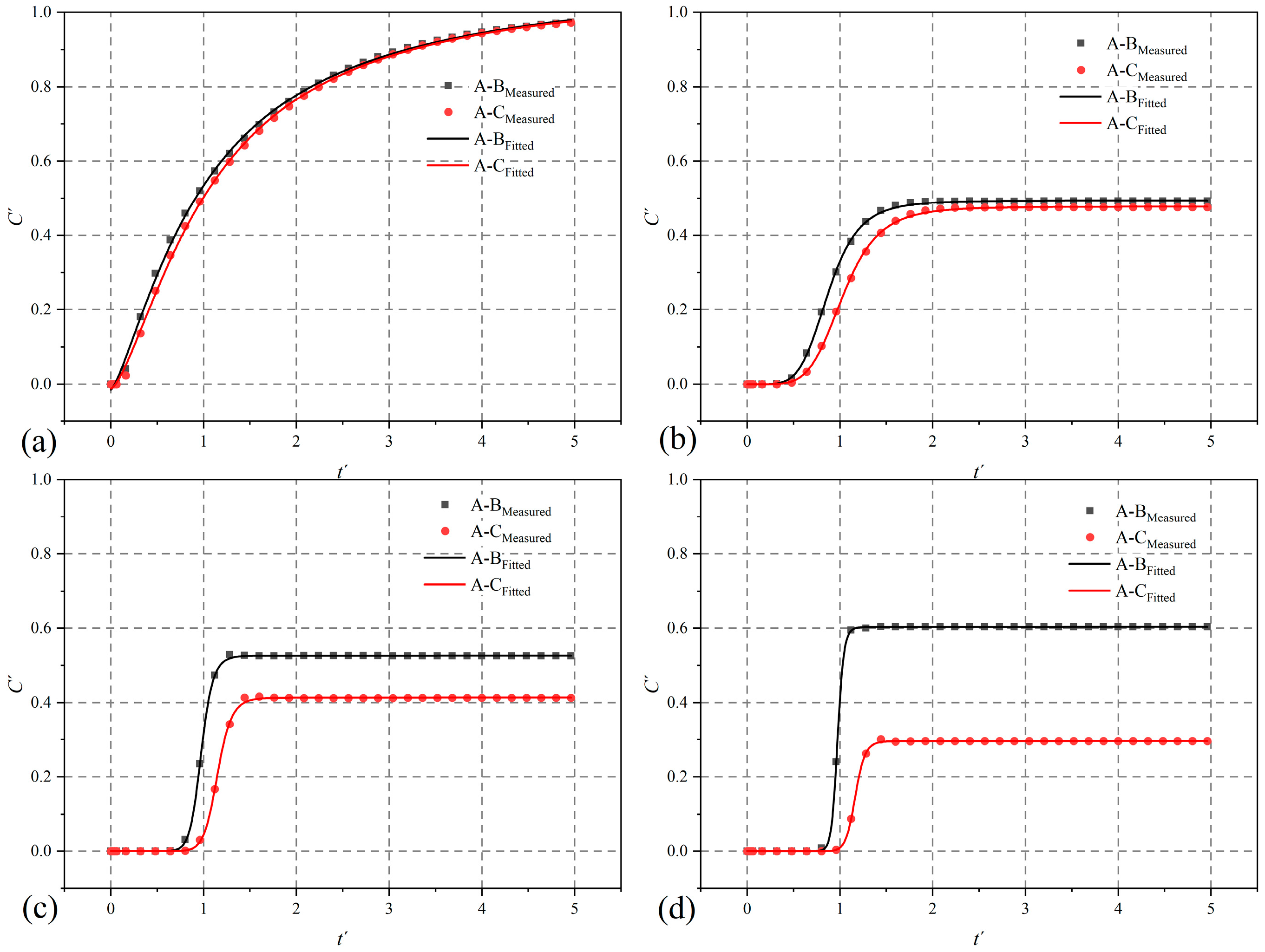
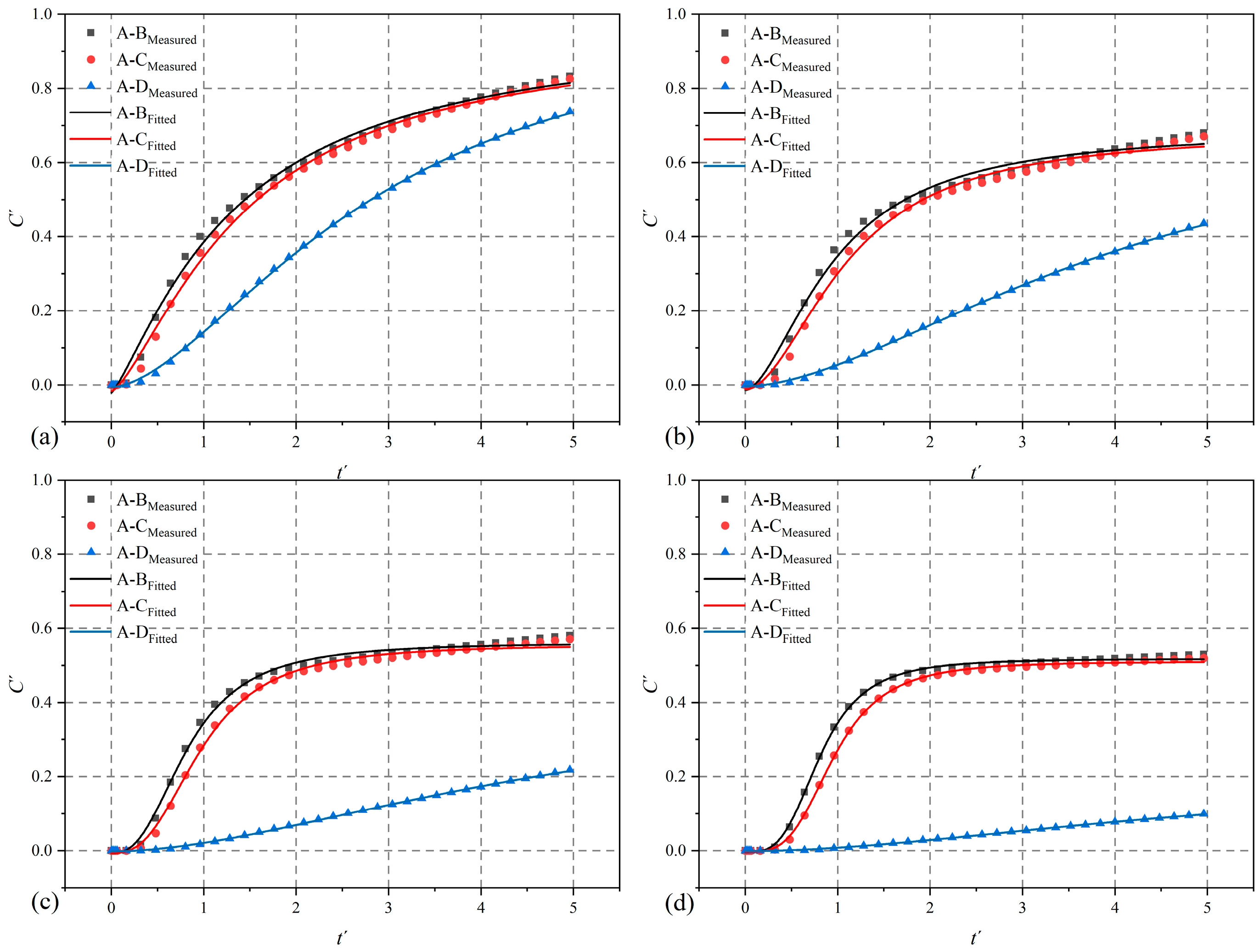
Figure 13 presents breakthrough curves (BTCs) at boundaries B and C for different Pe. Taking JRC = 17.5, Pe = 1, 10, 100, and 600 as an example, the transient variations of the normalized mean solute concentration at the outflow boundaries B and C were investigated.
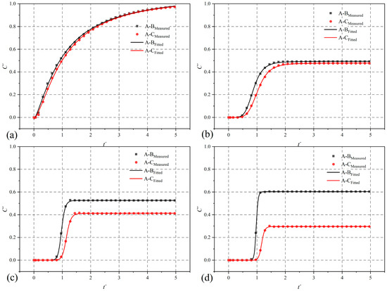
Figure 13.
Breakthrough curves at boundaries B and C for different Pe when JRC = 17.5: (a) Pe = 1; (b) Pe = 10; (c) Pe = 100; (d) Pe = 600.
For Pe = 1, the at boundaries B and C were around 1 at 5, and the mean solute concentration remained relatively the same throughout the process. For Pe = 10, the at boundaries B and C were close to 0.5 at 5, and thereafter, the difference between of boundaries B and C gradually increased with increasing Pe. After Pe increased to 100, the at boundaries B was 0.52, while at boundaries C was 0.41. For Pe = 600, the solute concentration difference between boundaries B and C was 0.31 and tended to stabilize with increasing Pe. From the above analysis, it can be seen that the solute transport process showed a typical flowrate-dependent.
It is also evident from the BTCs for all the Pe cases that there was a large deviation in at 5 when Pe = 1 and 10. The for boundaries B, C, and D was investigated when Pe was between 1 and 10. The BTCs of boundaries B, C, and D at Pe= 2, 3, 4, and 5 were analyzed to investigate the trend of the curves. When Pe= 2, the trends of for the three boundaries were nearly the same, and their value was around 0.8 at 5. With Pe increasing, the at boundaries B and C slowly decreased to about 0.5, and the at boundary D sharply decreased until close to 0. At this time, the BTCs at Pe = 5 was already nearly the same as those at Pe = 10. The above analysis revealed that the trend of BTCs when Pe was between 1 and 10 was significantly different from that when Pe was greater than 10. The main reason for this difference is that when the flowrate was very small, the influence of fluid flow and convection on solute transport was weak, and molecular diffusion played a dominant role in solute transport. In the solute transport process controlled by molecular diffusion, the solute was transported from the region of high concentration to the region of low concentration, i.e., it flowed in from the inlet, and diffused out uniformly to the three outlets. With increasing Pe, mechanical dispersion gradually replaced molecular diffusion in solute transport. The solute was gradually influenced by convection effect, the solute flowed from boundary A, redistributed at the intersection of the fractures and then flowed to boundaries B and C, and the solute flowing to boundary D was reduced by fluid obstruction until it approached 0. The mixing of solute at the intersection of the fracture will be discussed specifically in Section 4.4 Solute Mixing.
4.3.2. Effect of JRC
Figure 14 presents breakthrough curves (BTCs) at boundaries B and C for different JRC when Pe = 600. Taking Pe = 600, JRC = 2.5, 7.5, 12.5, and 17.5 as an example, the effects of surface roughness on solute breakthrough were investigated.
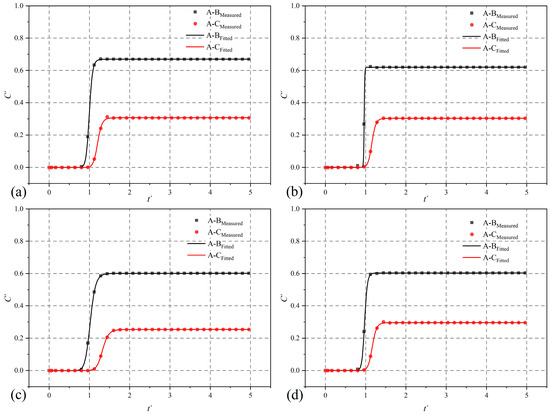
Figure 14.
Breakthrough curves at boundaries B, C, and D for different Pe when Pe = 600: (a) JRC = 2.5; (b) JRC = 7.5; (c) JRC = 12.5; (d) JRC = 17.5.
The BTCs under different surface roughness present consistency, both in the course of the curves and in the final stabilized achieved. The concentration difference between boundaries B and C decreased slightly with increasing JRC. Only from the results presented by the BTCs, the surface roughness of crossed fractures had a weak effect on solute breakthrough. In conjunction with the research in Section 4.2.2, it can be seen that the surface roughness affected the distribution of the concentration field only by changing the local aperture at the intersection and had a weak effect on the results of the solute breakthrough process.
4.4. Solute Mixing
To quantitatively characterize the solute transport process in crossed fractures, the mixing ratio was used in this study to describe the degree of solute mixing at the fracture crossings, defined as [14,16,19,26,46,47]
where C2 and C3 are the mean concentrations at the outlets on branches 2 and 3, respectively. In this equation, the researcher only considered the average concentration of solutes flowing into branches 2 and 3 after crossing through the fracture and did not consider the concentration of solutes flowing into branch 4. The definition of the mixing ratio shows that the mixing ratio is the transfer probability of the plasmas at the intersection of the fracture. The solute flowed from branch 1 and mixed at the fracture crossings due to convection and diffusion, thus flowing into branches 2, 3, and 4. As the fluid flow rate continued to increase, the fluid convection at the fracture crossings increased and the concentration of the solute flowing into each branch varied. Solute breakthrough in Section 4.3 showed that when Pe was greater than 10, convection of the fluid controled at this point at the fracture crossings and solutes were transported with the streamline route. When Pe was less than 10, the effect of molecular diffusion of the solute was not negligible at this point. Figure 15 shows that when Pe was less than 2, the concentration of solute flowing out of the three branches remained nearly the same. At this point, if Equation (7) continues to be used, it cannot accurately describe the probability of solute transfer to each outlet at the intersection of the fracture, resulting in errors in the mixing ratio at low concentrations. Therefore, Equation (7) was improved to conform to the numerical simulation at significant low flow rate, which is defined as
where C2, C3, and C4 are the mean concentrations at the outlets on branches 2, 3, and 4, respectively.
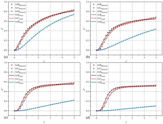
Figure 15.
Breakthrough curves at boundaries B, C, and D for different Pe when JRC = 17.5: (a) Pe = 2; (b) Pe = 3; (c) Pe = 4; (d) Pe = 5.
The crossed fractures with JRC = 17.5 and inlet combination 1 was used as the study object to calculate the mixing ratios for Pe of 0.1, 1, 2, 3, 4, 5, 6, 7, 8, 10, 100, and 600, as shown in Figure 16. Comparing the present study with previous similar studies, the mixing ratio curves are also plotted in Figure 16 [14,16,19,20,28]. The first three in Figure 16 were two-dimensional models that did not consider the effect of fracture surface roughness, and their results were significantly lower compared to this study. The fourth model considered a three-dimensional roughness fracture but did not consider the influence of size effect. This three-dimensional model had a low roughness and a uniform distribution, the fluid had a strong ability to pass through, and the stabilization of the mixing ratio was achieved at a low Pe. The fifth model, although it took into account the non-homogeneity of the cavity structure due to shear deformation and the differences in the overflow capacity of each branch, had a higher mixing ratio curve compared to each result due to its small size and the disproportionate influence caused by shear effects.
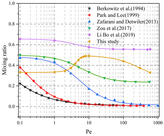
Figure 16.
Comparison of the mixing ratio as a function of Pe [14,16,19,20,28].
None of the five models mentioned previously considered the molecular diffusion of solutes at lower Pe, resulting in similar trends in the mixing ratio curves across these models. In this study, an improved mixing ratio equation was applied, fully accounting for the role of molecular diffusion in solute transport. At low Pe, the mixing ratio curves initially stabilized near 1/3, as molecular diffusion dominated solute transport. During this phase, the solute diffused uniformly into branches 2, 3, and 4 at the fracture intersection. As Pe increased, the convective effect of the fluid on solute transport became more pronounced. When Pe = 10, convection began to dominate, and the solute was almost entirely prevented from being transported to branch 4. For Pe > 10P, the trends of the mixing ratio curves aligned closely with those from other research models, further validating the accuracy of the improved equation. The final stabilized mixing ratio values were consistent with the results from the fourth model and higher than those from the first three models, reflecting the phenomenon of enhanced mixing due to surface roughness. This study demonstrated that the degree of solute mixing at fracture intersections was influenced by molecular diffusion, convection effects, and model roughness. At low Pe, molecular diffusion played the dominant role in determining the mixing ratio. However, as Pe increased, the influence of molecular diffusion diminished, and fluid convection became the controlling factor.
5. Conclusions
In this study, we investigated fluid flow and solute transport in 3D crossed fracture models, focusing on two key factors: the Péclet number (Pe) and the Joint Roughness Coefficient (JRC). Fracture surfaces were generated using a MATLAB code developed based on the improved SRA method, which allows for the construction of fracture surfaces with predetermined roughness. These surfaces were then imported into COMSOL to construct crossed fracture models and perform numerical simulations. The evolution of fluid flow and solute transport behavior in crossed fractures was quantitatively analyzed in relation to fracture surface roughness and Pe, providing insights into the impact of these parameters on transport dynamics.
Some general conclusions are summarized as follows:
(1) Channeling flow behavior: The channeling flow at fracture intersections became more pronounced with increasing Pe and JRC. As Pe increased from 1 to 600, the number of channeling flow streamlines rose, and the area of occurrence expanded. Similarly, as JRC increased from 2.5 to 7.5, 12.5, and 17.5, surface roughness significantly influenced fracture geometry and local aperture variations at the intersection. These changes affected the curvature of flow streamlines and the distribution of channeling flow.
(2) Concentration field evolution: The evolution of the concentration field was influenced by Pe, while its distribution was affected by JRC. For Pe < 1, solute transport was dominated by molecular diffusion. When 1 < Pe < 10, the transport process transitioned to a complete mixing mode. For Pe > 10, solute transport followed streamlines, and the streamline routing mode became dominant. As JRC increased from 2.5 to 7.5, 12.5, and 17.5, surface roughness affected the concentration field distribution by altering local aperture variations at the intersection.
(3) Solute breakthrough process: The solute breakthrough process revealed that Pe determined the trend of breakthrough concentration curves (BTCs), while the effect of JRC was relatively minor. For Pe = 1, the BTCs at two boundaries reached approximately 1 after 5 units of time. For Pe = 10, the BTCs at two boundaries were around 0.5 at the same time, with the difference increasing as Pe rose. At Pe = 100, the difference stabilized. Further analysis indicated that at low Pe, solute transport was controlled by molecular diffusion. BTCs under varying surface roughness exhibited consistency in both the shape of the curves and the final stabilized values.
(4) Solute mixing at fracture intersections: The degree of solute mixing at fracture intersections was influenced by molecular diffusion, convection, and surface roughness. For Pe < 10, molecular diffusion predominantly determined the mixing ratio. As Pe increased, the influence of molecular diffusion diminished, and fluid convection became the controlling factor. Based on these findings, the solute mixing equation was improved to better reflect the combined effects of molecular diffusion and convection.
In this study, we systematically examined the evolution of fluid flow and solute transport in 3D crossed fracture models under varying Pe and JRC and proposed an improved calculation method for solute mixing. However, this work focused exclusively on two simple orthogonal intersecting rough fractures. The apertures of the two fractures were constant, and the inflow−outflow boundary conditions for each branch were set to the same values. In natural fractured rock systems, factors such as variable aperture, intersection angles, fracture lengths, flow rate ratios between inflow branches, and flow types differ due to the variability of geo-hydraulic conditions in different regions. Understanding how these factors influence fluid flow and solute transport processes is a crucial area for future research. Additionally, in investigating solute mixing at significantly low flow rates, this study characterized the transition from molecular diffusion dominance to mechanical dispersion dominance. Future research should focus on identifying the critical point of this transition to further refine the description and understanding of the solute mixing process.
In our future study, the factors that influence the fluid flow and solute transport mechanisms will be investigated in depth. The first step is to obtain the key influencing factors through parameter identification by theoretical analysis. Then, the evolution relation of the influencing factors will be obtained through single-factor analysis. After that, the multiple regression variable algorithm will be utilized to construct the prediction equations of fluid flow and solute transport processes. Meanwhile, we will promote this research through experimental studies incorporating 3D printing technology. Firstly, computer-generated fracture surfaces will be fabricated into solid cross-fracture models using 3D printing technology. Subsequently, a seepage experimental platform will be constructed using a peristaltic pump, fluid pulse damper, and differential pressure transmitter. Finally, the crossed fracture model will be experimentally studied for fluid flow and solute transport using the seepage experimental platform.
Author Contributions
X.H., investigation, formal analysis, writing—original draft preparation, data curation, software, and validation; K.X., conceptualization, methodology, data curation, supervision; S.Z., formal analysis, software, and validation. All authors have read and agreed to the published version of the manuscript.
Funding
This study was funded by the National Natural Science Foundation of China (No. 2023YFC3804204 and No. 52374147) and the Chinese Postdoctoral Science Foundation (No. 2024M753531).
Data Availability Statement
The data that support the findings of this study are available from the corresponding author upon request.
Conflicts of Interest
The authors declare no conflict of interest.
References
- Neuman, S.P. Trends, prospects and challenges in quantifying flow and transport through fractured rocks. Hydrogeol. J. 2005, 13, 124–147. [Google Scholar] [CrossRef]
- Berkowitz, B. Characterizing flow and transport in fractured geological media: A review. Adv. Water Resour. 2002, 25, 861–884. [Google Scholar] [CrossRef]
- Chang, C.M.; Ni, C.F.; Li, W.C.; Lin, C.P.; Lee, I.H. Quantitation of the uncertainty in the prediction of flow fields in-duced by the spatial variation of the fracture aperture. Eng. Geol. 2022, 299, 106568. [Google Scholar] [CrossRef]
- Viswanathan, H.S.; Ajo-Franklin, J.; Birkholzer, J.T.; Carey, J.W.; Guglielmi, Y.; Hyman, J.D.; Karra, S.; Pyrak-Nolte, L.J.; Rajaram, H.; Srinivasan, G.; et al. From fluid flow to coupled processes in fractured rock: Recent advances and new frontiers. Rev. Geophys. 2022, 60, e2021RG000744. [Google Scholar] [CrossRef]
- Birdsell, D.T.; Rajaram, H.; Dempsey, D.; Viswanathan, H.S. Hydraulic fracturing fluid migration in the subsurface: A review and expanded modeling results. Water Resour. Res. 2015, 51, 7159–7188. [Google Scholar] [CrossRef]
- Pan, J.-B.; Lee, C.-C.; Yeh, H.-F.; Lin, H.-I. Application of fracture network model with crack permeability tensor on flow and transport in fractured rock. Eng. Geol. 2010, 116, 166–177. [Google Scholar] [CrossRef]
- Nong, R.; Wan, Y.; Ding, Y.; Chai, M.; Zhu, L. Effects of root systems on crack formation: Experiments, modeling, and analyses. Soil Tillage Res. 2023, 233, 105784. [Google Scholar] [CrossRef]
- Klyuev, R.V.; Brigida, V.S.; Lobkov, K.Y.; Stupina, A.A.; Tynchenko, V.V. On the issue of monitoring crack formation in natu-ral-technical systems during earth surface displacements. MIAB. Min. Inf. Anal. Bull. 2023, 11, 292–304. [Google Scholar]
- Berkowitz, B. Analysis of fracture network connectivity using percolation theory. J. Int. Assoc. Math. Geol. 1995, 27, 467–483. [Google Scholar] [CrossRef]
- Kosakowski, G.; Berkowitz, B. Flow pattern variability in natural fracture intersections. Geophys. Res. Lett. 1999, 26, 1765–1768. [Google Scholar] [CrossRef]
- Philip, J.R. The fluid mechanics of fracture and other junctions. Water Resour. Res. 1988, 24, 239–246. [Google Scholar] [CrossRef]
- Wilson, C.R.; Witherspoon, P.A. Flow interference effects at fracture intersections. Water Resour. Res. 1976, 12, 102–104. [Google Scholar] [CrossRef]
- Xu, C.; Dowd, P. A new computer code for discrete fracture network modelling. Comput. Geosci. 2010, 36, 292–301. [Google Scholar] [CrossRef]
- Berkowitz, B.; Naumann, C.; Smith, L. Mass transfer at fracture intersections: An evaluation of mixing models. Water Resour. Res. 1994, 30, 1765–1773. [Google Scholar] [CrossRef]
- Johnson, J.; Brown, S. Experimental mixing variability in intersecting natural fractures. Geophys. Res. Lett. 2001, 28, 4303–4306. [Google Scholar] [CrossRef]
- Park, Y.; Lee, K. Analytical solutions for solute transfer characteristics at continuous fracture junctions. Water Resour. Res. 1999, 35, 1531–1537. [Google Scholar] [CrossRef]
- Stockman, H.W.; Johnson, J.; Brown, S.R. Mixing at fracture intersections: Influence of channel geometry and the Reynolds and Peclet Numbers. Geophys. Res. Lett. 2001, 28, 4299–4302. [Google Scholar] [CrossRef]
- Wang, Z.; Xie, H.; Li, C.; Wen, X. Examining fluid flow and solute transport through intersected rock fractures with stress-induced void heterogeneity. Eng. Geol. 2022, 311, 106897. [Google Scholar] [CrossRef]
- Zafarani, A.; Detwiler, R.L. An efficient time-domain approach for simulating Pe-dependent transport through frac-ture intersections. Adv. Water Resour. 2013, 53, 198–207. [Google Scholar] [CrossRef]
- Zou, L.; Jing, L.; Cvetkovic, V. Modeling of flow and mixing in 3D rough-walled rock fracture intersections. Adv. Water Resour. 2017, 107, 1–9. [Google Scholar] [CrossRef]
- Mourzenko, V.V.; Yousefian, F.; Kolbah, B.; Thovert, J.F.; Adler, P.M. Solute transport at fracture intersections. Water Resour. Res. 2002, 38, 1–14. [Google Scholar] [CrossRef]
- Hull, L.C.; Koslow, K.N. Streamline routing through fracture junctions. Water Resour. Res. 1986, 22, 1731–1734. [Google Scholar] [CrossRef]
- Berkowitz, B.; Braester, C. Solute transport in fracture channel and parallel plate models. Geophys. Res. Lett. 1991, 18, 227–230. [Google Scholar] [CrossRef]
- Robinson, J.W.; Gale, J.E. A laboratory and numerical investigation of solute transport in discontinuous fracture systems. Groundwater 1990, 28, 25–36. [Google Scholar] [CrossRef]
- Wendland, E.; Himmelsbach, T. Transport simulation with stochastic aperture for a single fracture—Comparison with a laboratory experiment. Adv. Water Resour. 2002, 25, 19–32. [Google Scholar] [CrossRef]
- Stockman, H.W.; Li, C.; Wilson, J.L. A lattice-gas and lattice Boltzmann study of mixing at continuous fracture Junc-tions: Importance of boundary conditions. Geophys. Res. Lett. 1997, 24, 1515–1518. [Google Scholar] [CrossRef]
- Grubert, D. Effective dispersivities for a two-dimensional periodic fracture network by a continuous time random walk analysis of single-intersection simulations. Water Resour. Res. 2001, 37, 41–49. [Google Scholar] [CrossRef]
- Li, B.; Liu, R.; Jiang, Y. Influences of hydraulic gradient, surface roughness, intersecting angle, and scale effect on nonlinear flow behavior at single fracture intersections. J. Hydrol. 2016, 538, 440–453. [Google Scholar] [CrossRef]
- Moreno, L.; Tsang, Y.W.; Tsang, C.F.; Hale, F.V.; Neretnieks, I. Flow and tracer transport in a single fracture: A stochastic model and its relation to some field observations. Water Resour. Res. 1988, 24, 2033–2048. [Google Scholar] [CrossRef]
- Thompson, M.E.; Brown, S.R. The effect of anisotropic surface roughness on flow and transport in fractures. J. Geophys. Res. 1991, 96, 21923–21932. [Google Scholar] [CrossRef]
- Jia, C.; Huang, T.; Yao, J.; Xing, H.; Zhang, H. Effect of isolated fracture on the carbonate acidizing process. Front. Earth Sci. 2021, 9, 2296–6463. [Google Scholar] [CrossRef]
- Hu, Y.; Xu, W.; Zhan, L.; Ye, Z.; Chen, Y. Non-fickian solute transport in rough-walled fractures: The effect of contact area. Water 2020, 12, 2049. [Google Scholar] [CrossRef]
- Zou, L.; Cvetkovic, V. Impact of normal stress-induced closure on laboratory-scale solute transport in a natural rock fracture. J. Rock Mech. Geotech. Eng. 2020, 12, 732–741. [Google Scholar] [CrossRef]
- Brown, S.R. Fluid-Flow through Rock Joints—The Effect of Surface-Roughness. J. Geophys. Res.-Solid. 1987, 92, 1337–1347. [Google Scholar] [CrossRef]
- Mandelbrot, B. How long is the coast of britain? Statistical self-similarity and fractional dimension. Science 1967, 156, 636–638. [Google Scholar] [CrossRef]
- Barnsley, M.F.; Devaney, R.L.; Mandelbrot, B.B.; Peitgen, H.O.; Saupe, D.; Voss, R.F.; Saupe, D. Algorithms for random fractals. In The Science of Fractal Images; Springer New York Inc.: New York, NY, USA, 1988; pp. 71–136. [Google Scholar] [CrossRef]
- Liu, R.; He, M.; Huang, N.; Jiang, Y.; Yu, L. Three-dimensional double-rough-walled modeling of fluid flow through self-affine shear fractures. J. Rock Mech. Geotech. Eng. 2020, 12, 41–49. [Google Scholar] [CrossRef]
- Liu, H.-H.; Bodvarsson, G.S.; Lu, S.; Molz, F.J. A corrected and generalized successive random additions algorithm for simulating fractional levy motions. J. Int. Assoc. Math. Geol. 2004, 36, 361–378. [Google Scholar] [CrossRef]
- Barton, N.; Choubey, V. The shear strength of rock joints in theory and practice. Rock Mech. Rock Eng. 1977, 10, 1–54. [Google Scholar] [CrossRef]
- Wang, Y.; Zhang, Z.; Ranjith, P.G.; Luo, Y. Water-gas flow in rough rock fractures: Insights from coupled triaxial compression experiments. Hydrogeol. J. 2022, 30, 1569–1581. [Google Scholar] [CrossRef]
- Karmakar, S.; Tatomir, A.; Oehlmann, S.; Giese, M.; Sauter, M. Numerical benchmark studies on flow and solute transport in geological reservoirs. Water 2022, 14, 1310. [Google Scholar] [CrossRef]
- De Dreuzy, J.R.; Méheust, Y.; Pichot, G. Influence of fracture scale heterogeneity on the flow properties of three-dimensional discrete fracture networks (DFN). J. Geophys. Res. Solid Earth 2012, 117, B11207. [Google Scholar] [CrossRef]
- Huang, N.; Liu, R.; Jiang, Y.; Li, B.; Yu, L. Effects of fracture surface roughness and shear displacement on geo-metrical and hydraulic properties of three-dimensional crossed rock fracture models. Adv. Water Resour. 2018, 113, 30–41. [Google Scholar] [CrossRef]
- Bodin, J.; Delay, F.; de Marsily, G. Solute transport in a single fracture with negligible matrix permeability: 2. mathematical formalism. Hydrogeol. J. 2003, 11, 434–454. [Google Scholar] [CrossRef]
- Bodin, J.; Delay, F.; de Marsily, G. Solute transport in a single fracture with negligible matrix permeability: 1. fundamental mechanisms. Hydrogeol. J. 2003, 11, 418–433. [Google Scholar] [CrossRef]
- Lee, S.H.; Kang, P.K. Three-Dimensional Vortex-Induced Reaction Hot Spots at Flow Intersections. Phys. Rev. Lett. 2020, 124, 144501. [Google Scholar] [CrossRef] [PubMed]
- Li, G. Tracer mixing at fracture intersections. Environ. Geol. 2002, 42, 137–144. [Google Scholar] [CrossRef]


Disclaimer/Publisher’s Note: The statements, opinions and data contained in all publications are solely those of the individual author(s) and contributor(s) and not of MDPI and/or the editor(s). MDPI and/or the editor(s) disclaim responsibility for any injury to people or property resulting from any ideas, methods, instructions or products referred to in the content. |
© 2024 by the authors. Licensee MDPI, Basel, Switzerland. This article is an open access article distributed under the terms and conditions of the Creative Commons Attribution (CC BY) license (https://creativecommons.org/licenses/by/4.0/).