Abstract
This study investigates the impact of natural gas pipeline leakage on the soil temperature field through numerical simulations. Physical and mathematical models were developed to analyze the temperature and flow field changes resulting from pipeline leaks. The study explores the influence of various leakage factors on the temperature distribution in the surrounding soil. Key findings include the identification of the buried pipeline temperature as a critical factor influencing the soil temperature gradient when surface temperatures are similar to the subsurface constant temperature. Upon leakage, the pressure distribution around the leak is symmetrical, with a higher pressure at the leak point, and the Joule–Thomson effect causes a rapid decrease in gas temperature, forming a permafrost zone. The study also reveals that increased transport pressure expands the permafrost area, with pressure playing a significant role in the temperature field distribution. Additionally, an increase in the leak orifice diameter accelerates the expansion of the permafrost area and reduces the time for temperature stabilization at monitoring points. Conversely, changes in the leak direction mainly affect the spatial distribution of the permafrost zone without significantly altering its size. The findings provide valuable insights for monitoring natural gas pipeline leaks through temperature field variations.
1. Introduction
As industrial development progresses, the demand for natural gas continues to rise, creating significant challenges in pipeline transportation. Among these challenges, natural gas pipeline leakage emerges as a particularly critical issue. In recent years, this issue has become a significant focus of research both domestically and internationally. Consequently, research on natural gas pipeline leakage is essential for preventing accidents and accurately predicting the spread of leaks.
Zhang Yuntao et al. [1] developed a diffusion model to simulate the spread of natural gas leakage from buried pipelines under varying wind speeds and investigated the impact of the wind speed on laser detection. Their results show that as the wind speed increases, the diffusion range of natural gas shifts upwind and closer to the ground, leading to a reduction in the gas concentration and affecting the accuracy of laser-based detection systems. Jin Hao et al. [2] proposed an acoustic model for detecting and locating natural gas pipeline leaks, which they experimentally validated. Their study notably improved the leak detection accuracy and localization by developing a high-pressure, long-distance circular pipeline simulation platform. This was further enhanced by an improved acoustic wave propagation speed formula and a dual-threshold denoising optimization method. Hou et al. [3] introduced a method for detecting and locating small natural gas leaks using extended Kalman filtering (EKF). They created a discrete model of transient pipeline flow and, by employing a virtual multi-point leakage model coupled with noise processing techniques, were able to accurately estimate both the leakage rate and the location of small leaks. Liu Cuiwei et al. [4] investigated a leak detection method based on dynamic pressure waves in natural gas pipelines. They designed an innovative leak detection model, and their experimental results demonstrated that this method significantly outperformed traditional techniques in terms of accuracy, with smaller errors, thus proving its reliability and potential for real-world application. Pan Xinghua et al. [5] developed a software-based method to enhance the accuracy of natural gas pipeline leak detection using non-isothermal modeling. The adaptive model in this method effectively estimated the leak locations, particularly under conditions of varying temperatures and pressure drops. Yang [6] utilized Fluent software (version 2024 R2) to simulate gas diffusion from natural gas pipeline leaks in urban environments. This research examined how various building parameters, such as the height-to-width ratio and building spacing, influence gas diffusion patterns and concentration distribution. The findings provide a theoretical foundation to aid rescue personnel in rapidly assessing hazardous areas after an accident. Hu [7] conducted numerical simulations to analyze gas diffusion from buried natural gas pipelines under different soil porosities and pipeline pressures. The study developed a correction equation for factors influencing the leakage volume and examined methane diffusion trends in various directions. Moreover, it established the relationship between the safety distance from the leak point and time. Liu [8] applied both experimental and numerical simulation methods to develop a model for calculating leakage rates and gas diffusion in subsea natural gas pipelines. The research examined the effects of pressure, leakage orifice size, and water depth on the leakage rate and diffusion process. The numerical model validated the accuracy of the gas leakage rate estimates, demonstrating that this method can effectively predict gas diffusion in subsea environments. Yao and others [9] proposed a natural gas pipeline leak detection model that combines acoustic feature processing and feature reconstruction techniques. After evaluating the performance of this method on the GPLA-12 dataset, they found that the fault identification accuracy rate was as high as 95.17%. Li and others [10], through on-site localization of underground natural gas pipeline leak points at a testing station, found that the micro-TOFMS method could more efficiently and accurately locate natural gas pipeline leaks.
To effectively recognize pipeline signals under different operating conditions, Li and others [11] proposed an integrated leak detection method based on Singular Value Decomposition, Variational Mode Decomposition, and Probabilistic Neural Networks, demonstrating through experiments that this method achieved a 100% accuracy rate in distinguishing between leak and non-leak signals. Miao and others [12] proposed a pipeline leak detection method based on unsupervised learning and pressure sensing. Their study showed that this method could distinguish between normal and leak conditions, as well as assess the risk and severity of leaks. Zhu and others [13] proposed a pipeline leak detection method based on an improved Variational Mode Decomposition algorithm and Lempel–Ziv complexity analysis, finding that this method had a higher classification accuracy rate compared to other methods. To assess the accuracy of estimating leak locations along gas transmission pipelines, it is necessary to consider measurement uncertainties. Chen and others [14] used the Monte Carlo method to analyze the impact of various factors on leak location estimation. Their research found that the manual measurement of the pipeline length and the actual leak location played a crucial role in the uncertainty of leak location estimation. Feature extraction of pipeline signals is vital for detecting natural gas pipeline leaks. Lu and others [15] proposed a pipeline leak feature extraction method based on Variational Mode Decomposition and Local Linear Embedding. Their research found that this method could classify pipeline signals with an accuracy rate of up to 95%. Soil characteristics and surface conditions have a significant impact on the risk of underground natural gas pipeline leakage accidents. Bu and others [16] used numerical simulation to study the impact of surface conditions and soil characteristics on methane leak diffusion, and their direct calculation model of methane leakage rates filled a gap in calculating underground pipeline leakage rates under different soil characteristics.
Since natural gas comes into contact with soil, the environmental temperature of the soil around the leakage site also changes rapidly. As the environmental temperature of the area around the pipeline changes after a leak, it is possible to identify the pipeline leak location based on the physical phenomena accompanying natural gas pipeline leakage using a real-time monitoring distributed fiber optic temperature measurement system for gas pipeline leaks, thereby monitoring and issuing early warnings for pipeline leaks. However, current research on monitoring natural gas pipeline leaks using changes in the temperature field is not sufficient. Therefore, conducting related research on the impact of natural gas pipeline leakage on the temperature field is of great significance for monitoring natural gas leaks and accurately locating natural gas leak positions.
This study offers a novel approach by developing a refined numerical model that simulates the impact of natural gas pipeline leakage on the surrounding soil temperature field. Unlike previous studies, which typically focus on only one or two leakage factors, our model takes into account multiple parameters, including pipeline pressure, leak size, and distance from the leak, to provide a comprehensive understanding of the temperature distribution. Additionally, we explore the formation and growth of permafrost around the pipeline, which has not been thoroughly studied. By addressing the nonlinear effects of these leakage factors on the temperature field, this research answers the critical question of how gas pipeline leaks affect the soil temperature over time, especially in terms of the development of permafrost and the long-term environmental impact.
2. Model Establishment
2.1. Mathematical Model
Due to the interactions between molecules in natural gas and the non-negligible size of the molecules themselves, the Peng–Robinson (PR) equation is chosen as the state equation, as shown in Equation (1).
In Equation (1), P represents the gas pressure in Pascals (Pa); V is the molar volume of the gas in cubic meters per mole (m3/mol); T is the temperature in Kelvin (K); R is the gas constant in Joules per mole-Kelvin (J/(mol·K)); a and b are constants.
The following assumptions are made for the soil medium: the soil is considered an isotropic homogeneous porous medium; the spatial structure of the soil does not change during the mass transfer process; the effect of gravity on fluid flow in the porous medium is negligible; it is assumed that the soil pores are filled with air, and the moisture in the soil is ignored; the leaking natural gas does not react chemically with the surrounding soil. Based on these assumptions, the continuity equation is as shown in Equation (2), the motion equation as in Equation (3), the equation for uniform porous media as in Equation (4), and the mixed gas density as in Equation (5).
In Equation (5), is the mixed gas density in kilograms per cubic meter (kg/m3); t is time in seconds (s); ui represents the velocity of the mixed gas in the x, y, z directions in meters per second (m/s); ε is the soil porosity; p is the gas pressure in Pascals (Pa); is the dynamic viscosity of the gas in Pascal-seconds (Pa·s); Si is the source term of the momentum equation, where i = x, y, z; 1/ is the coefficient of viscous resistance in per square meter (1/m2); C2 is the coefficient of inertial resistance in per meter (1/m).
is the magnitude of velocity in meters per second (m/s); is the mass fraction of the component in percent (%). Ma is the relative molecular mass of air; Mv is the relative molecular mass of methane.
This study considers the compressibility of natural gas, with the RNG k-ε model chosen for the turbulence calculation model. After natural gas leaks from the pipeline and diffuses in the soil pores, it can be approximated as gas flowing in a pipe with an extremely small diameter. Assuming that natural gas is a single-component gas, the energy equation is as in the following Equation (6). The convective heat transfer mathematical model between natural gas and soil is expressed as in Equation (8).
In Equation (8), T is the soil temperature in Kelvin (K); ε is the soil porosity; ρg is the gas density in kilograms per cubic meter (kg/m3); ρs is the density of the soil solid in kilograms per cubic meter (kg/m3); Eg is the total energy of the gas in Joules (J); Es is the total energy of the soil solid in Joules (J); p is the gas pressure in Pascals (Pa); λg is the heat transfer coefficient of the gas in Watts per meter-Kelvin (W/m·K); λs is the heat transfer coefficient of the soil solid in Watts per meter-Kelvin (W/m·K); λeff is the heat transfer coefficient of the porous medium of the soil in Watts per meter-Kelvin (W/m·K); h is the convective heat transfer coefficient in Watts per square meter-Kelvin (W/m2·K); Ts is the soil temperature in Kelvin (K); Tg is the gas temperature in Kelvin (K).
Solving the heat transfer model requires the determination of the boundary conditions of the heat transfer model. The fluvial boundary conditions of the natural gas in the soil heat transfer model are shown in Figure 1.
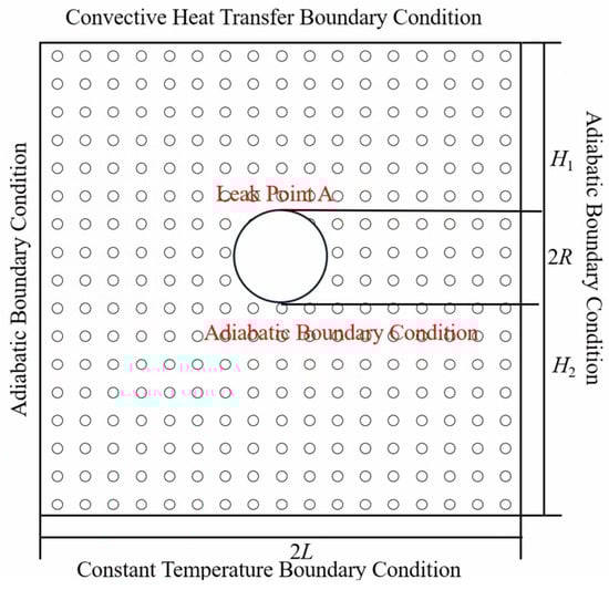
Figure 1.
Schematic of the heat transfer boundary conditions.
For natural gas and soil convective heat transfer, the convective heat transfer condition is as in Equation (10); when assuming the pipeline is well insulated and there is no heat exchange with the soil, the convective heat transfer condition is as in Equation (11); the temperature change in the horizontal direction at a distance from the coordinate origin is very small and can be ignored, as in Equation (12).
In the above equations, R is the radius of the gas pipeline in meters (m); H1 is the vertical distance from any point in the soil to the leak point in meters (m); h is the convective heat transfer coefficient between natural gas and soil in Watts per square meter-Kelvin (W/(m2·K)); H2 is the distance from the gas pipeline to the constant temperature layer in meters (m); Tc is the constant temperature of the soil layer in Kelvin (K); L is the distance from the pipeline to the soil adiabatic layer in meters (m).
2.2. Physical Model
Based on research, the commonly used sizes of natural gas pipelines in China are selected as 711 mm, 660 mm, 1016 mm, and 1219 mm in diameter. The leak aperture sizes are chosen as 1 mm, 2 mm, 4 mm, and 6 mm. The pipeline length is 10 m, buried at a depth of 1.5 m, with a wall thickness of 10 mm. The entire calculation area is 10 m × 10 m × 10 m. The physical model of the underground natural gas pipeline leakage includes three parts: the fluid inside the pipe, the fluid at the leak hole, and the soil fluid area. The physical model schematic is shown in Figure 2. The position of the leak hole has three different directions, located directly above, directly below, and on the side of the center of the pipeline.
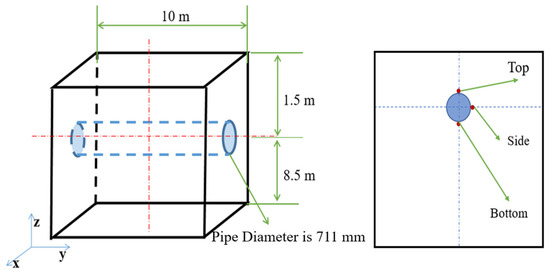
Figure 2.
Schematic of the physical model.
2.3. Mesh Division
The boundary naming situation of the physical model is as shown in Table 1. Since the size of the leak hole is much smaller compared to the overall size, a boundary layer of 5 layers is set, with a layer height growth rate of 1.1. The overall mesh drawing situation is shown in Figure 3. The skewness of the mesh is in the range of 0.4–0.5, and the minimum inverse orthogonality is greater than 0.2, which indicates that the quality of the drawn mesh is relatively good.

Table 1.
Boundary position and naming situation.
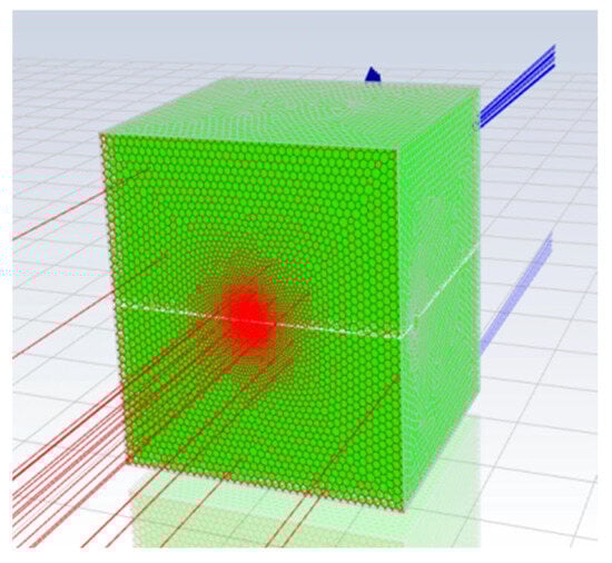
Figure 3.
Mesh division situation.
2.4. Mesh Independence Verification
Before conducting subsequent simulation calculations, it is essential to verify the mesh independence to eliminate the influence of the mesh on the required physical quantities and to ensure computational accuracy. For this purpose, 10 sets of meshes were established using the same physical model, and the mesh independence verification is shown in Table 2.
Table 2.
Mesh independence verification.
Observing Table 2, it can be seen that when the minimum cell size is greater than 1 mm (groups 1–3), the monitored physical quantities differ significantly from the subsequent seven groups, indicating that the minimum cell size of the mesh should not be set too large. The remaining seven groups show an average velocity at the leak orifice of 20.2199 m/s. Generally, a minimum inverse orthogonality quality greater than 0.2 is considered indicative of good mesh quality, and these seven groups meet this condition. It is observed that when the minimum cell size is less than 1 mm and the maximum cell size is less than 500 mm (groups 5–10), the values of the monitored physical quantities are close to the previously calculated average velocity at the leak orifice. Therefore, when the minimum cell size is less than 1 mm and the maximum cell size is less than 500 mm, the mesh has little effect on the calculation results.
Around the center of the natural gas pipeline, Figure 4 shows the temperature field distribution in the horizontal direction at the soil surface for different mesh sizes. It can be seen that the overall trends in temperature change calculated with four different numbers of meshes are basically consistent. The temperature differences at this point under different mesh sizes are relatively small. Considering both the computation time and accuracy, a mesh size of 0.025 m with a total of 4,625,847 elements was chosen for the temperature field study.
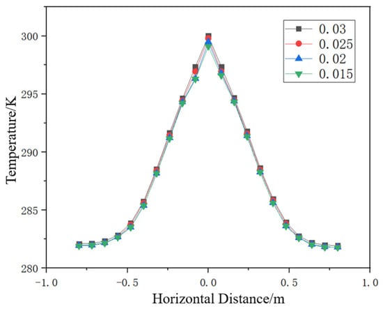
Figure 4.
Temperature field distribution in the soil surface in the horizontal direction for different mesh sizes.
3. Numerical Results of the Temperature Field
3.1. Results of the Flow Field and Temperature Field Due to Natural Gas Pipeline Leakage
Considering the possibility of varying degrees of leakage in buried gas pipelines, 21 different leakage scenarios were simulated. The pipeline is laid at a depth of 1.5 m from the surface, and the parameters of the natural gas pipeline are as shown in Table 3.
Table 3.
Parameters of the natural gas pipeline.
When the buried natural gas pipeline is operating normally without leakage, the temperature field is in a steady state. The temperature field distribution in the soil on the YZ plane under different ambient temperatures is shown in Figure 5, and on the XY plane in Figure 6. Observing from the YZ plane, there is a small temperature gradient along the pipeline direction, and with the increase in ambient temperature, air convection causes the temperature above the soil to increase.
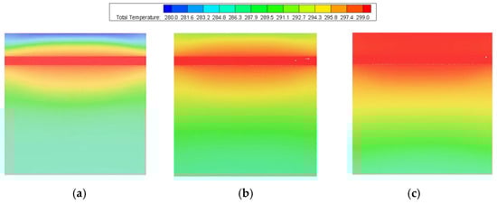
Figure 5.
Soil temperature distribution under different ambient temperatures (YZ plane). (a) Ambient temperature 280 K, (b) ambient temperature 290 K, (c) ambient temperature 300 K.
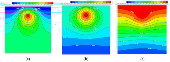
Figure 6.
Soil temperature distribution under different ambient temperatures (XY Plane). (a) Ambient temperature 280 K, (b) ambient temperature 290 K, (c) ambient temperature 300 K.
On the XY plane, it can be observed that the soil temperature distribution is symmetrical, i.e., the soil temperature is the same at the same distance from the gas pipeline wall. When the surface temperature is lower than the constant temperature of the underground layer, the isotherms around the buried natural gas pipeline show a convex distribution; when the surface temperature is close to the constant temperature of the underground layer, the temperature of the buried gas pipeline is an important factor determining the gradient of the soil temperature field; when the surface temperature is higher than the constant temperature of the underground layer, the isotherms around the buried natural gas pipeline show a concave distribution. Therefore, before pipeline leakage, the ambient temperature determines the temperature gradient around the buried pipeline.
When the natural gas pipeline leaks, the temperature field is in a transient state. At the leak orifice, the Joule–Thomson effect occurs, which is the phenomenon where the temperature of the gas changes due to irreversible adiabatic expansion as it passes through a porous medium.
With a gas leak orifice diameter of 4 mm and leakage direction at 12 o’clock, and a soil temperature of 278 K, the temperature field distribution in the soil after 30 s of leakage at a pipeline pressure of 4 MPa is shown in Figure 7. From the temperature cloud diagram, it can be seen that due to the aforementioned Joule–Thomson effect, a throttling effect occurs near the leak orifice, causing a rapid drop in gas temperature and the formation of a permafrost area. When the natural gas first leaks, the gas gathers at the leak orifice and contacts the soil. Since the thermal conductivity of the soil is much lower than that of natural gas, poor heat transfer occurs nearby, forming a permafrost area, and as time goes on, the gas continues to diffuse, causing the permafrost area to expand, eventually leading to an overall decrease in the soil temperature.
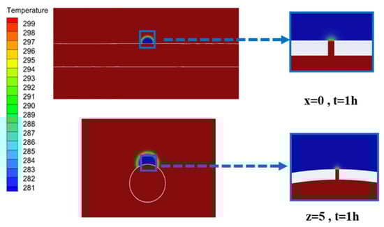
Figure 7.
Temperature cloud diagram at a pipeline outlet pressure of 4 MPa.
The pressure cloud diagram at a pipeline outlet pressure of 4 MPa is shown in Figure 8. The natural gas pressure near the leak orifice decreases due to the outflow of gas from the pipeline, forming a negative pressure area. The size and shape of this negative pressure area depend on the flow rate of the leaking gas and the porosity and permeability of the soil around the leak orifice. The natural gas pressure away from the leak orifice returns to atmospheric pressure. The isotropic nature of the soil results in a symmetrical distribution of pressure in the horizontal direction centered on the leak orifice.
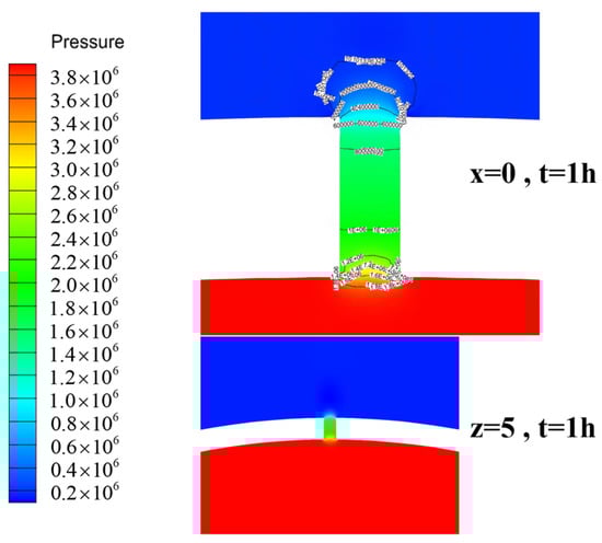
Figure 8.
Pressure cloud diagram at a pipeline outlet pressure of 4 MPa.
The velocity cloud diagram and velocity vector diagram at a pipeline outlet pressure of 4 MPa are shown in Figure 9. From Figure 9, it can be seen that the velocity distribution contours inside and outside the pipeline near the leak orifice are radial. The velocity distribution is symmetrical around the leak orifice, with the velocity magnitude at the orifice significantly higher than in other areas. For buried pipelines, soil resistance reduces the speed of gas entering the soil. When the pressure behind the gas balances the soil resistance in front, the velocity reaches a stable state.
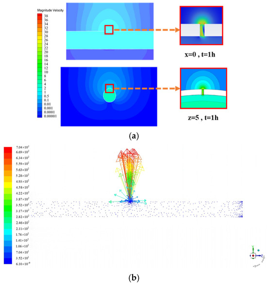
Figure 9.
(a) Velocity cloud diagram at a pipeline outlet pressure of 4 MPa; (b) velocity vector diagram.
3.2. Results of the Sensor Monitored Temperature with Time Variation
Using finite element numerical analysis software, a leakage model consistent with the temperature field model was established, resulting in an accurate and reliable leakage simulation model. The layout design of the sensor monitoring points is shown in Figure 10. Combining finite element analysis and simulation, the layout of the temperature monitoring points was determined. The temperature sensors were arranged from No. 1 to No. 8. Monitoring point No. 1 is located 100 mm above the leak orifice, and point No. 2 is 200 mm above it. Similarly, points No. 3 and No. 4 are placed 300 mm and 400 mm above the leak orifice, respectively. Other monitoring points are shown in Figure 10. The Report Definitions module was used to set the location of the monitoring points and the parameters to be monitored, recording the soil temperature near the outlet.
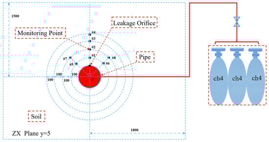
Figure 10.
Distribution of temperature sensor monitoring points in the soil.
Based on the working conditions given in Table 3, Case 14, and the positions of the sensors in Figure 10, the coordinates of each monitoring point were calculated as shown in Table 4 for subsequent analysis.
Table 4.
Coordinates of temperature sensor monitoring points.
Figure 11 shows the temperature changes over time for four monitoring points #1~4. The results indicate that the temperature at monitoring point #1 begins to slowly decrease at 13 s, reaching a minimum temperature of 267 °C and maintaining stability. The temperature at monitoring point #2 begins to decrease at 332 s, and the time to reach a stable minimum temperature of 268 °C increases. The temperature at monitoring point #3 begins to decrease at 1382 s, while point #4 takes even longer to sense temperature changes, at 3122 s.
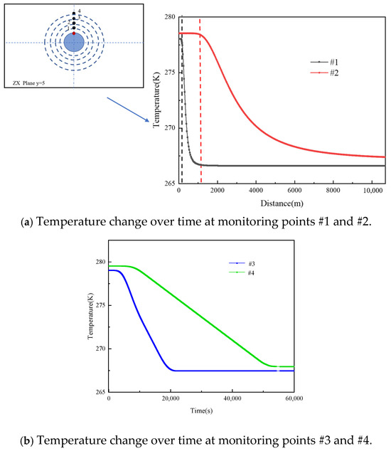
Figure 11.
Temperature change over time at monitoring points #1 to #4.
A further analysis of the temperature changes over time for monitoring points #1~4 reveals the initial sensing time and the time taken to reach a stable temperature at different points. These values were then fitted with the distance of each monitoring point from the leak orifice, allowing for a comprehensive analysis of the pattern of soil temperature changes following a natural gas leak. Figure 12a shows the relationship between the initial sensing time and the distance of the monitoring points, and Figure 12b shows the relationship between the time taken to reach stability and the distance of the monitoring points.
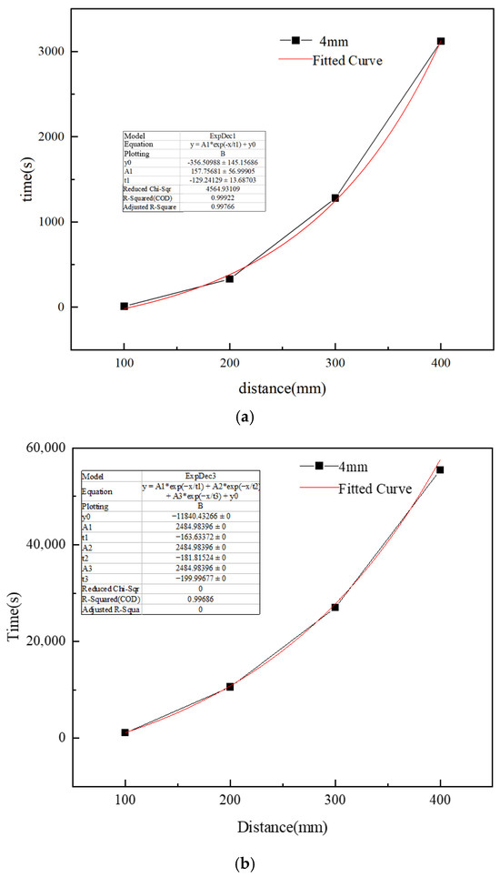
Figure 12.
Relationship between time and distance at monitoring points. (a) Relationship between initial sensing time and monitoring point distance, (b) relationship between time taken to reach stability and monitoring point distance.
As shown in Figure 11 and Figure 12, the time required for temperature changes to be sensed and to stabilize nonlinearly increases with the distance of the monitoring points from the leak orifice. The final stable temperature at each monitoring point is the temperature of the permafrost layer.
Figure 13 shows the temperature and time changes at three monitoring points, #1, 5, and 6. The results are consistent with those previously described and as shown in Table 5, indicating a significant difference in the initial sensing times between points #5 and #6 compared to point #1, despite all being located on the same arc 100 mm from the pipeline’s outer diameter.
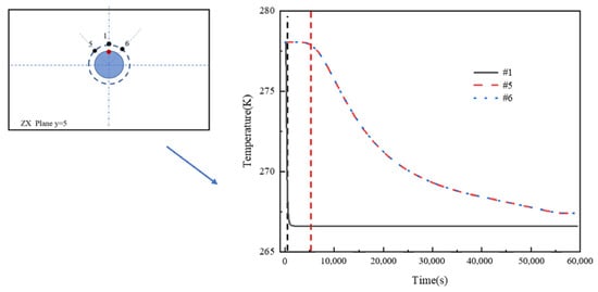
Figure 13.
Temperature change over time at monitoring points #1, 5, and 6.
Table 5.
Initial sensing times at monitoring points #1, 5, and 6.
Figure 14 shows the temperature and time changes at three monitoring points, #2, 7, and 8. Table 6 delineates a marked disparity in the initial sensing times between monitoring points 7 and 8 in contrast to point 2, notwithstanding their collocation along the same arcuate segment 200 mm from the pipeline’s outer diameter. The symmetry of the soil temperature distribution around the leak orifice contributes to the consistency in temperature changes over time for points #7 and #8.
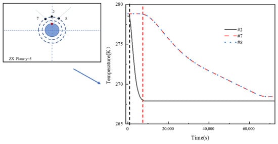
Figure 14.
Temperature change over time at monitoring points #2, 7, and 8.
Table 6.
Initial sensing times at monitoring points #2, 7, and 8.
Through temperature sensors at different locations, the temperature distribution of the soil above buried natural gas pipelines can be analyzed, which is helpful for designing and optimizing the pipeline’s cooling system. Furthermore, real-time monitoring of temperature changes in the soil above buried pipelines can help in the early detection of leaks, thereby enhancing pipeline safety.
4. Effects of Different Leakage Factors on the Temperature Field
4.1. Pipeline Outlet Pressure
For a natural gas pipeline with a diameter of 711 mm, which is buried at a depth of 1.5 m and insulated by a 10 mm-thick polyurethane layer (disregarding the pipeline’s inherent thickness), the internal fluid temperature is maintained at 300 K. The pipeline features a leak orifice with a diameter of 4 mm and an internal fluid velocity of 7 meters per second. Simulations were performed in an anemically neutral environment, encompassing diverse leakage scenarios across a spectrum of pipeline outlet pressures. A comprehensive analysis and comparative data evaluation were undertaken for Cases 1 through 6 as detailed in Table 3, with the resultant pressure profiles under varying pipeline outlet pressures graphically represented in Figure 15. Additionally, the velocity distribution of the fluid under different outlet pressures is delineated in Figure 16.
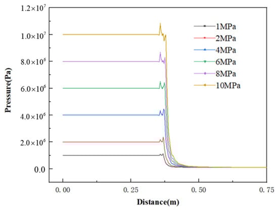
Figure 15.
Soil pressure distribution under different pipeline outlet pressures.
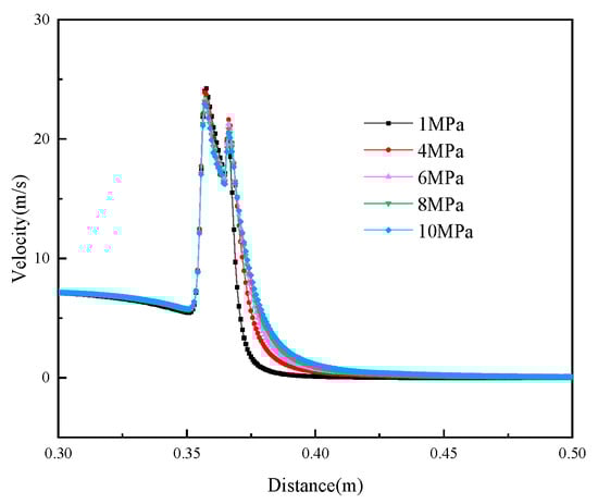
Figure 16.
Fluid velocity distribution under different pipeline outlet pressures.
As shown in Figure 17, a natural gas pipeline leak leads to heat removal from the surrounding environment. Due to poor heat transfer in the soil, the heat around the leak orifice is difficult to disperse to other areas, causing the expansion of the permafrost area near the leak orifice as the gas transport pressure increases. In order to calculate the minimum temperature within the permafrost region under various pipeline outlet pressures for the prediction of safety issues in actual production, a further analysis of Figure 17 was conducted. This analysis yielded the relationship between the minimum temperature in the permafrost region and different pipeline outlet pressures, as illustrated in Figure 18.
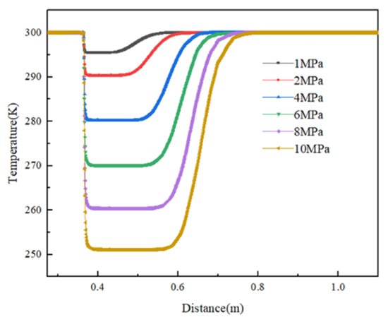
Figure 17.
Soil temperature distribution under different pipeline outlet pressures.
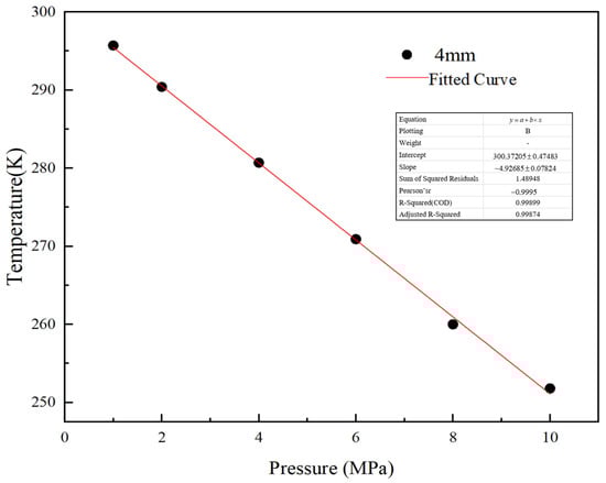
Figure 18.
Relationship between lowest temperature in permafrost layer and pressure.
As shown in Figure 19, at the initial stage of the leak, the gas speed decreases with increasing pipeline outlet pressure; however, after passing through the soil, the gas speed increases with increasing outlet pressure. Overall, higher pipeline outlet pressures result in faster gas flow during leakage, leading to a larger diffusion range of the gas in the leakage area.
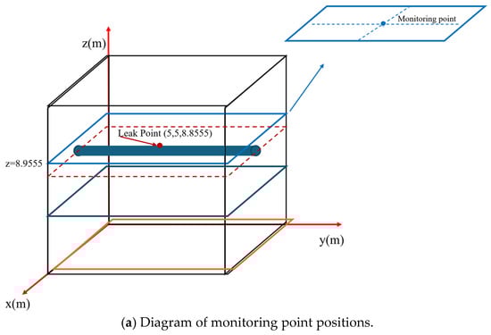
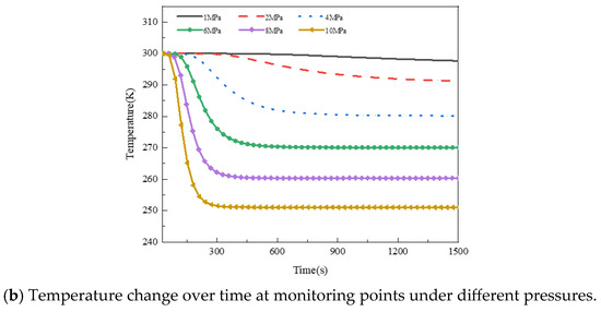
Figure 19.
Temperature change over time at monitoring points under different pressures.
4.2. Leak Orifice Diameter
Simulations were conducted for different leak orifice diameters under the conditions outlined in Table 3 and Cases 4 and 7–9. The velocity distributions under different leak orifice diameters along the central line are shown in Figure 20.
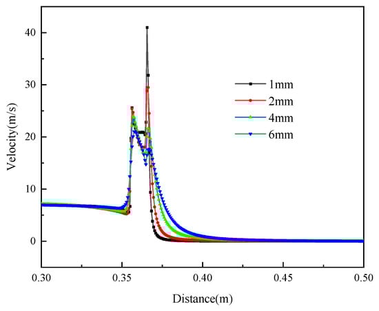
Figure 20.
Fluid velocity distribution along the central line under different leak orifice diameters.
As shown in Figure 20, at the initial stage of the leak, the gas speed is lower for larger leak orifices, but after passing through the soil, the gas speed increases with the size of the leak orifice. A larger leak orifice results in a faster gas speed in the soil, as the orifice size affects the pressure drop at the pipeline outlet, accelerating the gas flow and increasing the leak rate.
Figure 21 shows that the permafrost area in the soil expands with the size of the leak orifice. The leak orifice size does not change the temperature of the permafrost area but affects the rate at which cold gas flows, as well as the area of the leak, leading to faster diffusion of the leaking gas into the soil.
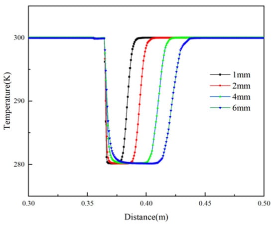
Figure 21.
Soil temperature distribution along the central line under different leak orifice diameters.
From Figure 22a, it is evident that larger leak orifices lead to faster temperature changes at the monitoring points, and the time to reach stability is shorter. This is due to the increased diffusion speed of natural gas in the soil caused by larger leak orifices, allowing the gas to more easily spread into the soil, increasing the diffusion range and ultimately lowering the sensed temperature, stabilizing at the lowest temperature of the permafrost area. This correlates with the observations in Figure 21. Overall, it is considered that the leak orifice diameter is a significant factor in the changes to the surrounding temperature field following a natural gas pipeline leak.
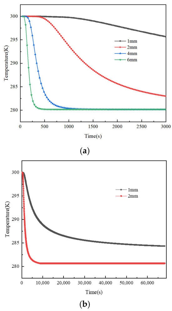
Figure 22.
Temperature change over time at monitoring points under different leak orifice sizes. (a) Temperature change over time at monitoring points under different leak orifice sizes, (b) diagram of monitoring point positions.
4.3. Different Leakage Directions
For a buried natural gas pipeline with a diameter of 711 mm, buried at a depth of 1.5 m, and insulated with a 10 mm thick polyurethane layer (ignoring the pipeline’s own thickness), the internal fluid temperature is 300 K, with a pipeline outlet pressure of 4 MPa, a small hole diameter of 4 mm, and an internal fluid flow speed of 7 m/s. Simulations were conducted in a no-wind environment for different leakage directions. Analysis and data comparison for Cases 3 and 13 in Table 3 were conducted, resulting in soil temperature cloud diagrams under different leakage directions, as shown in Figure 23. The direction of the leak mainly affects the location of the permafrost area in the soil, with little impact on the size of the permafrost area; it also indicates that different leakage directions affect the temperature field of the soil near the gas pipeline, but the impact on the soil temperature in areas far from the pipeline is negligible.
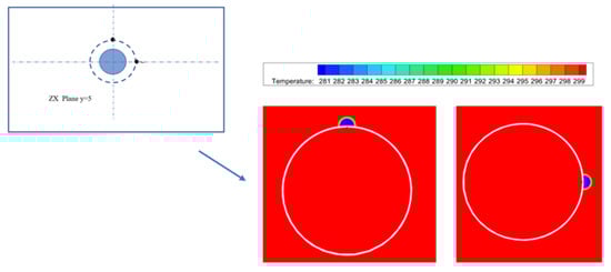
Figure 23.
Soil temperature cloud diagrams under different leakage directions.
4.4. Different Pipeline Diameters
For a buried natural gas pipeline with a depth of 1.5 m, insulated with a 10 mm thick polyurethane layer (ignoring the pipeline’s own thickness), the internal fluid temperature is 300 K, with a pipeline outlet pressure of 6 MPa, a small hole diameter of 6 mm, and an internal fluid flow speed of 7 m/s. Simulations were conducted in a no-wind environment for different pipeline diameters. An analysis and data comparison for Cases 12, 17, and 21 in Table 3 were conducted, resulting in soil temperature cloud diagrams on the XZ section for different pipeline diameters, as shown in Figure 24. The temperature distributions along the central line for different pipeline diameters are shown in Figure 25. Combined with the temperature cloud diagrams and temperature curves, it can be observed that different pipeline diameters under the same pressure and leak orifice diameter have little impact on the temperature of the permafrost area.
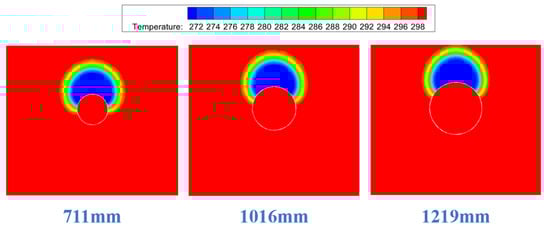
Figure 24.
Range of influence diagrams for different pipeline diameters (XZ section).
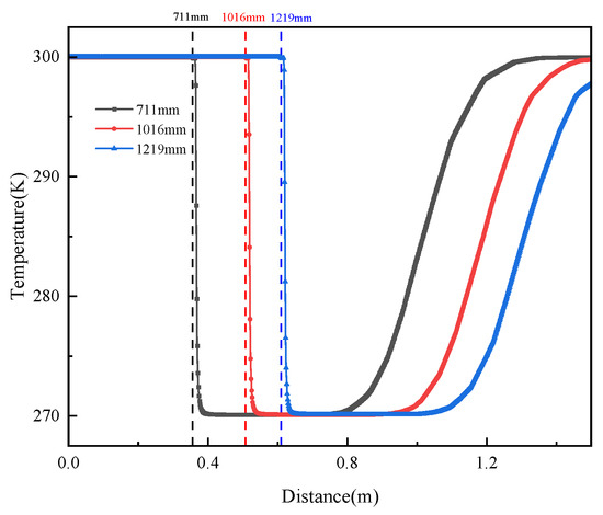
Figure 25.
Soil Temperature distribution along the central line under different pipeline diameters.
5. Conclusions
This paper uses numerical simulation methods to calculate the impact of natural gas pipeline leakage on the soil temperature field, establishing corresponding physical and mathematical models. The effects of natural gas pipeline leakage on the flow and temperature fields were analyzed, as well as the pattern of temperature change over time at monitoring points. The impact of different leakage factors on the temperature field was studied, leading to the following conclusions:
1. When the surface temperature is lower than the underground constant temperature layer, the isotherms around the buried pipeline are convex. As the surface temperature approaches the constant layer, the pipeline temperature becomes a key factor for the soil temperature gradient. When the surface temperature is higher, the isotherms become concave.
2. After a pipeline leak, pressure is symmetrically distributed around the leak, with higher pressure at the leak point. The velocity distribution near the leak is radial, and the Joule–Thomson effect causes a rapid temperature drop, forming a permafrost area.
3. As the distance from the leak increases, the time for temperature changes to stabilize increases nonlinearly. The monitoring points at a 45° angle take longer to sense temperature changes compared to vertical points at the same distance.
4. Increasing the pipeline outlet pressure expands the permafrost area, and the lowest temperature in the permafrost layer is linearly related to the pressure. Pressure affects the temperature field distribution.
5. Increasing the leak orifice diameter expands the permafrost area and reduces the time for monitoring points to sense and stabilize temperature. The orifice size has the greatest impact on the permafrost area range.
6. The leakage direction affects the location of the permafrost area but has little effect on its size or the soil temperature far from the pipeline.
7. The diameter of the pipeline has little impact on the size of the permafrost area under the same pressure and leak orifice diameter.
6. Discussion and Recommendations
This study highlights the significant impact of natural gas pipeline leakage on the surrounding soil temperature field, with effects largely governed by pressure, leakage orifice size, and soil thermal properties. The rapid cooling near the leak point, driven by the Joule–Thomson effect, results in a permafrost zone that expands due to the soil’s limited heat conductivity. Increased pipeline pressure and larger leakage orifices accelerate gas diffusion and enlarge the permafrost zone, emphasizing their importance in temperature field dynamics. The symmetrical pressure and velocity distributions around the leak point and the nonlinear relationship between distance and temperature stabilization time underscore the critical role of soil characteristics and sensor placement in optimizing leakage monitoring systems. Additionally, while the leakage direction influences the permafrost positioning, the pipeline diameter plays a minimal role in determining the extent of the affected area.
To enhance the effectiveness of pipeline leakage monitoring and mitigation, it is recommended to optimize sensor placement by accounting for the symmetry and nonlinearity of temperature changes. Future pipeline designs should consider insulation systems that mitigate the formation and expansion of permafrost zones, especially under high-pressure conditions. Furthermore, real-time monitoring systems integrating soil porosity and thermal properties should be developed to improve the detection and response to leakage events. Extending simulations to include heterogeneous soil characteristics and long-term environmental impacts would provide more comprehensive insights and guide the development of robust, proactive leakage management strategies.
Author Contributions
Conceptualization, Z.X.; methodology, W.C.; writing—original draft, X.G.; data curation, X.Z. (Xin Zhang); software, X.Z. (Xiahua Zhang); visualization, W.C.; investigation, Z.G.; writing—review and editing, Z.X. All authors have read and agreed to the published version of the manuscript.
Funding
This research received no external funding.
Data Availability Statement
The datasets generated or analyzed during this study are available from the corresponding author upon reasonable request.
Conflicts of Interest
Author Xiahua Zhang was employed by Wuhan Marine Machinery Plant Co., Ltd., The remaining authors declare that the research was conducted in the absence of any commercial or financial relationships that could be construed as a potential conflict of interest.
References
- Zhang, Y.; Zhao, X.; Wang, S.; He, Z. Study of wind speed effect on laser detection in natural gas pipeline leaking. DEStech Trans. Mater. Sci. Eng. 2017. [Google Scholar] [CrossRef] [PubMed][Green Version]
- Jin, H.; Zhang, L.; Liang, W.; Ding, Q. Integrated leakage detection and localization model for gas pipelines based on the acoustic wave method. J. Loss Prev. Process Ind. 2014, 27, 74–88. [Google Scholar] [CrossRef]
- Hou, Z.; Zhu, X. An EKF-based method and experimental study for small leakage detection and location in natural gas pipelines. Appl. Sci. 2019, 9, 3193. [Google Scholar] [CrossRef]
- Liu, C.; Li, Y.; Fan, L.; Xu, M. Leakage monitoring research and design for natural gas pipelines based on dynamic pressure waves. J. Process Control 2017, 50, 66–76. [Google Scholar] [CrossRef]
- Pan, X.; Karim, M.N. Modelling and monitoring of natural gas pipelines: New method for leak detection and localization estimation. Comput. Aided Chem. Eng. 2015, 37, 1787–1792. [Google Scholar]
- Yang, J.; Zhang, J.-H.; Mei, S.; Liu, D.; Zhao, F. Numerical simulation of sudden gas pipeline leakage in urban block. Energy Procedia 2017, 105, 4921–4926. [Google Scholar] [CrossRef]
- Hu, M.; Li, H.; Chen, L.; Xie, P.; Zhang, Z.; Yang, M.; Wu, M.; Zhang, Q. Numerical simulation on the leakage and diffusion of the natural gas of the underground pipeline in the soil. J. Phys. Conf. Ser. 2021, 2083, 032082. [Google Scholar] [CrossRef]
- Liu, C.; Liao, Y.; Shaoxiong, W.; Li, Y. Quantifying leakage and dispersion behaviors for sub-sea natural gas pipelines. Ocean Eng. 2020, 216, 108107. [Google Scholar] [CrossRef]
- Yao, L.; Zhang, Y.; He, T.; Luo, H. Natural gas pipeline leak detection based on acoustic signal analysis and feature reconstruction. Appl. Energy 2023, 352, 121975. [Google Scholar] [CrossRef]
- Li, M.; Liu, B.; Chen, T.; Liu, R.; Guo, Y.; Hou, K. On-site leakage locating of underground natural gas pipeline based on Ne tracer by miniature time-of-flight mass spectrometry. Talanta 2023, 254, 124170. [Google Scholar] [CrossRef] [PubMed]
- Li, H.; Chu, L.; Lu, J.; Liu, Q.; Li, F.; Zhang, K. SVD-VMD algorithm and its application in leak detection of natural gas pipeline. Pet. Sci. Technol. 2022, 41, 230–255. [Google Scholar] [CrossRef]
- Xingyuan, M.; Hong, Z.; Zhaoyuan, X. Leakage detection in natural gas pipeline based on unsupervised learning and stress perception. Process Saf. Environ. Prot. 2023, 170, 76–88. [Google Scholar]
- Zhu, L.; Wang, D.; Yue, J.; Lu, J.; Li, G. Leakage detection method of natural gas pipeline combining improved variational mode decomposition and Lempel–Ziv complexity analysis. Trans. Inst. Meas. Control 2022, 44, 2865–2876. [Google Scholar] [CrossRef]
- Runchang, C.; Shan, C.; Yang, W.D.K.; Khoo, B.C. Modelling and quantification of measurement uncertainty for leak localisation in a gas pipeline. Meas. Sens. 2022, 24, 100443. [Google Scholar]
- Lu, J.; Fu, Y.; Yue, J.; Zhu, L.; Wang, D.; Hu, Z. Natural gas pipeline leak diagnosis based on improved variational modal decomposition and locally linear embedding feature extraction method. Process Saf. Environ. Prot. 2022, 164, 857–867. [Google Scholar] [CrossRef]
- Bu, F.; Chen, S.; Liu, Y.; Guan, B.; Wang, X.; Shi, Z.; Hao, G. CFD analysis and calculation models establishment of leakage of natural gas pipeline considering real buried environment. Energy Rep. 2022, 8, 3789–3808. [Google Scholar] [CrossRef]
Disclaimer/Publisher’s Note: The statements, opinions and data contained in all publications are solely those of the individual author(s) and contributor(s) and not of MDPI and/or the editor(s). MDPI and/or the editor(s) disclaim responsibility for any injury to people or property resulting from any ideas, methods, instructions or products referred to in the content. |
© 2024 by the authors. Licensee MDPI, Basel, Switzerland. This article is an open access article distributed under the terms and conditions of the Creative Commons Attribution (CC BY) license (https://creativecommons.org/licenses/by/4.0/).