Optimization of Ansys CFX Input Parameters for Numerical Modeling of Pump Performance in Turbine Operation

Abstract

The paper deals with the issue of determining the optimal setting of input variables in Ansys CFX for modeling pump flow in turbine operation (PAT). The pump model was created in Autodesk Inventor. The mesh for numerical simulations was created using Ansys Fluent Meshing, considering the mesh quality parameters’ skewness and aspect ratio. The Ansys CFX computational model was experimentally verified on an actual pump by measuring the performance parameters on a test circuit and using the PIV (particle image velocimetry) method. The research indicated that the most suitable setting for the model input variables was the inlet pressure and PAT flow rate combination. Another option was to adjust the pressure at the pump inlet and outlet. However, the calculation time in this case was up to 30% longer. The comparison of the model results with the experiment showed that the deviations in the numerical model performance values did not exceed 10% of the values measured on the test circuit. Only the calculated torque was 1.2 ± 0.13 Nm higher on average than the torque measured on the test circuit. This difference is most likely due to the simplification of the geometry of the computational mesh in order to reduce the computation time.

1. Introduction

This paper addresses the issue of pumps operating in turbine mode (PAT). It focuses on predicting performance parameters using a mathematical model and simulation of fluid flow in Ansys. The optimization of the Ansys CFX setup for five different combinations of input variables is verified experimentally. The results are validated using the PIV method and by measuring the performance characteristics on the test circuit. The results are a comparison of the different settings.

In the REPowerEU 2022 plan, in line with the Green Deal, EU countries have committed to achieving at least 45% renewable energy in total consumption by 2030 through energy efficiency and product eco-design improvements. One way to achieve this goal is to use the energy potential of small hydropower (SHP) more efficiently [1]. Considering the budget of SHP projects, hydroturbines are the most expensive item. A more cost-effective alternative is a pump as turbine (PAT), which can replace conventional small hydroturbines [2]. A PAT is a pump operating in reverse mode, where pressurized water is fed through the discharge pipe to spin the impeller and electric motor that serves as a power generator. Systems using pumps in turbine mode have existed since the third decade of the 20th century [3]. PATs can also be used for energy storage when they operate, similarly to pumped storage hydropower plants.

The most significant advantages of PATs are their simple design and easy maintenance. Due to mass production, the pumps are readily available in terms of price and spare parts. In addition, PAT can be used for pressure control in water distribution systems (WDS) or similar infrastructures such as irrigation, wastewater, or sewerage systems. In all these cases, PAT can replace pressure-reducing valves [4], the use of which results in energy losses. Due to the tendency to use all energy sources efficiently, PAT is becoming a solution for energy recovery [5,6,7]. Some studies report that up to 40% of energy can be recovered this way [8,9]. Other sources indicate that the return on investment in this sector can range from 4 to 10 years, depending on the degree of sophistication of the automatic control system [10]. In order to achieve the best possible device efficiency, the pump to be operated in reverse mode must be selected very carefully. The optimal operation of PAT is less efficient than that of a conventional turbine. Therefore, knowing the pump’s performance characteristics is essential when selecting a pump for a particular application. Manufacturers usually do not have information on the characteristics of the pump in turbine mode; hence, the need arises to determine them in some way. The problem of transforming pump characteristics to PAT was addressed recently by Barbarelli et al. [11] and Polák [12,13]. A large number of formulas exist for recalculating PAT performance parameters. Most are based only on the conversion based on the pump efficiency optimum (BEP). However, PAT often operates outside the BEP, so knowing the complete performance characteristics is useful.

Bogdanović-Jovanović et al. [14] mentioned several ways of recalculation in their paper and stated that the deviation of the calculated values is around 10% or lower. Thus, the exact recalculation of the pump’s characteristics, design and selection for turbine operation for the given site-specific conditions is still an open issue. The most reliable method of obtaining PAT characteristics is by measurement on a test circuit. However, this is often not possible for various reasons, such as time, material, and financial. An alternative is the recalculations mentioned above, which quickly and simply give an idea of the basic PAT parameters, but with limited accuracy. Another option is a wide range of calculation programs that can produce performance characteristics and other outputs, such as velocity and pressure fields or streamlines throughout the PAT flow profile in a relatively short time. One of the most prominent and robust leaders in this field is Ansys, namely, Ansys CFX and Ansys Fluent applications.

The use of a numerical flow model, specifically the Ansys CFX module, to generate PAT performance characteristics and their subsequent comparison was addressed by many authors, for example, Nasir et al. [15]. They also dealt with various modifications to the impeller, such as increasing the number of impeller blades, reducing the blade thickness, rounding the blade tips and adjusting the angle at the inlet of the blade. Sun-Sheng et al. [16] investigated the use of PAT impeller splitter blades. They concluded that the splitter blades positively affect efficiency and head reduction. They conducted their research using Ansys CFX and compared it with measured values. The CFX values were, on average, 4% higher than the measured values. Yang et al. [17] investigated the effect of PAT variable shaft speeds and also compared the results with Ansys CFX. Again, the CFX model values were about 10% higher than the measured values. Nowadays, with the rise of artificial intelligence, deep learning methods such as large language models (LLMs) and Kolmogorov–Arnold networks (KAN) are emerging. These can also be used for performance characteristic prediction. In the pump domain, these methods were used by Peng et al. [18,19]. However, they have not yet been applied to radial centrifugal pumps.

Zariatin et al. [20] concluded that surface roughness has a greater effect on PAT performance than on a pump. Specifically, a change in roughness to 0.16 μm achieved by fine grinding or polishing will improve PAT performance by up to 13% over the original impeller. Stejskal et al. [21] also addressed the surface roughness of pump impellers and spiral casings. Bade et al. [22] dealt with the effect of the roundness of the trailing edge of the blades and the surface roughness of both the spiral casing and impeller. They found that an increase of 70 μm in the roughness of the spiral casing and impeller reduced the efficiency by up to 4%. They used Ansys Fluent for the simulations. It is essential to mention that surface roughness is usually left in the “universal” mode for most simulations, and is therefore one of the simplifying assumptions for the computational modules. Other authors, such as Nandan et al. [23] and Tchada et al. [24], also addressed the radial centrifugal pump and PAT simulation using Ansys. Different variables were specified as model input parameters for the studies mentioned above. The most commonly used were pressure, flow rate, fluid velocity at the turbine inlet, and pressure or flow rate at the turbine outlet.

2. Materials and Methods

2.1. Numerical Model of PAT Flow

For the numerical simulations, a 3D model of the pump was created in Inventor according to the technical specifications supplied by the manufacturer. The model included impeller flow sections, spiral casings, a connecting 200 mm long draft tube, and a 150 mm long supply pipe. The model was further modified (simplified) for simulations in Ansys CFX. The reason for this was the significantly higher computational demand. Simplification included omission of the roughness, volumetric and mechanic losses, geometry simplification, and the type of Ansys calculation module. In Ansys Fluent Meshing, a fine tetrahedron mesh with approximately 1.1 million elements was created to meet the quality parameters of aspect ratio with a minimum value of 0.15 and skewness parameter with a maximum value of 0.65. These two parameters ensured that the model mesh was of sufficient quality and ready for simulations. In order to capture the most important phenomena, the mesh was refined to the orbital region. Further refinement was applied to the impeller blades and the spiral tongue, as well as to the transitions between the draft tube and the impeller and the spiral (see Figure 1). A sensitivity analysis of the mesh was also performed. Several meshes with different element sizes were created to optimize the mesh and capture the observed phenomena.

The simulation was set as a steady state. For the individual parts, the material from the Ansys library “water” was chosen without considering heat transfer, and for the turbulence model, k-epsilon. The value of y+ ranged up to 250. A full wheel was simulated. For this reason, a “frozen rotor” was used as an interface, and the “specified pitch angle” was set to 360°. The steady-state values of head, moment, and efficiency were monitored in the simulation.

As part of the numerical model optimization, five different combinations of input parameters were created and compared (

Table 1. Combination of input variables for individual simulations.

Setting Number	Parameter at PAT Input	Parameter at PAT Output
1	pressure	flow rate
2	flow rate	pressure
3	pressure	pressure
4	pressure	pressure = 0
5	velocity	flow rate

). The pressure and flow combinations are the most commonly chosen input parameters for pump and turbine simulations. The authors mentioned above used these input variables either with particular values or with zero draft tube pressure. In rare cases, the PAT inlet velocity combined with the PAT outlet flow rate are chosen as input parameters [25].

The last input variable that was the same in all settings was shaft speed. These ranged from 600 to 2300 rpm. For each combination of input and output parameters, seven sub-simulations corresponding to seven points of measured performance characteristics were run simultaneously with seven points of PIV velocity field measurements. The input parameters for the simulations were the values from the measurements on the test circuit (see

Table 2. Measured values on the test circuit and input values for Ansys simulations.

n-Shaft Speed [rpm]	ps-Pressure [kPa]	pp-Pressure [kPa]	Q-Flow Rate [l/s]	M-Torque [Nm]
2381	−1.17	127.61	4.32	0.22
2098	−2.12	123.67	5.08	1.31
1794	−2.24	119.00	5.62	2.17
1503	−1.94	116.84	5.95	2.79
1202	−1.11	114.31	6.25	3.33
897	0.05	114.85	6.37	3.70
607	0.86	114.68	6.50	3.86

). Subsequently, the results of the simulations were compared with the results measured on the PAT during the performance tests. Specifically, the turbine head (H_t), torque (M_t) and PAT efficiency (η_t) were compared. Other outputs of the numerical model were the velocity fields in the inlet pipe and the pressure course in the spiral casing and impeller. These outputs were compared with the results of the PIV measurements in the draft tube.

2.2. Test Circuit

Experimental verification was carried out on an actual PAT on a hydraulic circuit in the Fluid Mechanics Laboratory at the Faculty of Engineering of the Czech University of Life Sciences Prague. The circuit diagram is presented in Figure 1. The test circuit consisted of two tanks with pipes, control and measuring components. The feed pump (FP) generated the turbine’s hydropower potential, and water flowed in the direction of the red arrows when valve V₂ was closed. The water flow was measured using a SITRANS FM MAG 5100 W (Siemens, Munich, Germany) electromagnetic flowmeter (Q) (0.5% accuracy). The pressures at the p_p and p_s points were measured with HEIM 3340 pressure sensors (0.5% accuracy) installed according to Class 1 accuracy requirements [26]. Turbine output and speed were measured by a dynamometer (D) with a Magtrol TMB 307/41 speed and torque sensor (0.1% accuracy). The LSLV0055s100-4EOFNS (LS Electric, Gyeonggi-do, Korea) frequency inverter allowed continuous speed control of the PAT shaft.

A META Plus 5 single-stage radial centrifugal cast iron pump with spiral casing was used for the experiment. The schematic of the pump and its performance parameters guaranteed by the manufacturer are presented in Figure 2. Seven measurements were taken at a head of 13 m to obtain the performance characteristics of the PAT. The measurements were based on the standard EN ISO 9906 [26] for testing hydrodynamic pumps. For each point of the performance characteristic, the velocity field in the draft tube was simultaneously recorded using the PIV method.

2.3. PIV Measurement of Velocity Fields

A 2D PIV kit from TSI was used to measure the fluid velocity fields in the PAT draft tube (see Figure 3). The basis was a dual-pulse Nd:YAG laser (YAG100-100-LIT) with a wavelength of 532 nm working with a Light Sheet Optics 610,026 and a Powerview Cameras 630,092 camera. The setup was complemented by a LaserPulse Model 610,036 synchronizer and a PIV 600054-64 COMPUTER with INSIGHT™ 4G-2DTR Data Acquisition software. Hollow 100-SLVR glass spheres with a diameter of 12 μm were dispersed in the flowing fluid, silver-coated to increase light reflection on the surface.

A vertical plane in the axis of the transparent draft tube at the PAT outlet was chosen to monitor the fluid velocity fields (see Figure 3). For measurement purposes, a laser was placed above the pipe to produce a pair of consecutive flashlight sections in the pipe with a time interval of 50 μs. A high-speed camera placed perpendicular to the plane scanned the area of the flashlight sections synchronously with the light flashes. The camera output was pairs of images recording the positions of the fluorescent particles. The first image (t) shows the initial positions of the particles during the first flash, and the second image (t’) shows the final positions during the second flash. The image processing was performed by specialized software, which determined the directions and magnitudes of the flowing fluid’s velocity vectors by comparing the particles’ positions in the pairs. Scilab software (v6.1.1) was used to visualize the measured data. In this program, the graphical form of the vector fields was created, as presented in the following section.

3. Results and Discussion

The various settings in Ansys gave very similar results in the converged solutions. The streamlines were almost identical in all cases: the velocity vectors were mostly in the same direction, but had different magnitudes in each setting. Three parameters were monitored in the Ansys calculations, namely, turbine head, torque, and total PAT efficiency. Their curves are shown in Figure 4, Figure 5 and Figure 6. The program had difficulty converging at the highest shaft speed (2400 rpm) in all settings. This increased the calculation time up to double. Setting 5 proved complicated, with a drop-in pressure value of up to 100 kPa from the measured value at higher speeds. However, the shapes of the streamlines in the converged solutions were consistent with the PIV results. From 1800 rpm onwards, some of the observed variables failed to converge. Even so, the head was similar to the other settings. However, this setting cannot be recommended, given the significant inaccuracy of the calculated pressures and the convergence problem. The model results were consistent with the experiment in settings 3 and 4, where both inlet and outlet pressure values were used as input variables, the model results were consistent with the experiment. In setting 3, the measured pressures, both at the turbine inlet and outlet, were used as input variables. The main difference was the computation time. In setting 3, it was, on average, 15% longer than in settings 1 and 2. In the case of setting 4, where zero pressure in turbine outlet was set as an input parameter, the simulation time was up to 30% longer than for the other simulations.

Despite the different pressure values for all calculations in all settings, very satisfactory agreement of turbine head values was achieved. Figure 4 shows a graph of turbine head versus shaft speed. The blue curve shows the head H measured on the test circuit modified by volume losses for a more accurate comparison with the calculated values. The separate points are the head values calculated for simulations 1 to 5. The calculated head values were up to 2 m smaller than the measured values at lower shaft speed. Conversely, they were up to 3 m higher at higher shaft speed. For values close to BEP, the difference between calculation and experiment was around 0.5 m, i.e., less than 4%.

Figure 6 shows a graph of the dependence of torque on shaft speed. The points dotted along the curve are the M_t values measured on the test circuit modified by mechanical losses for a more accurate comparison with the calculated values. The separate points show the torque values calculated in Ansys according to settings 1 to 5. The comparison shows that all calculated values were significantly higher than the measured values, on average, by 1 ± 0.12 Nm. The cause of these deviations is probably the different roughness of the flow parts, the type of Ansys calculation module chosen, and the simplification of the geometry of the flow parts in the creation of the 3D models.

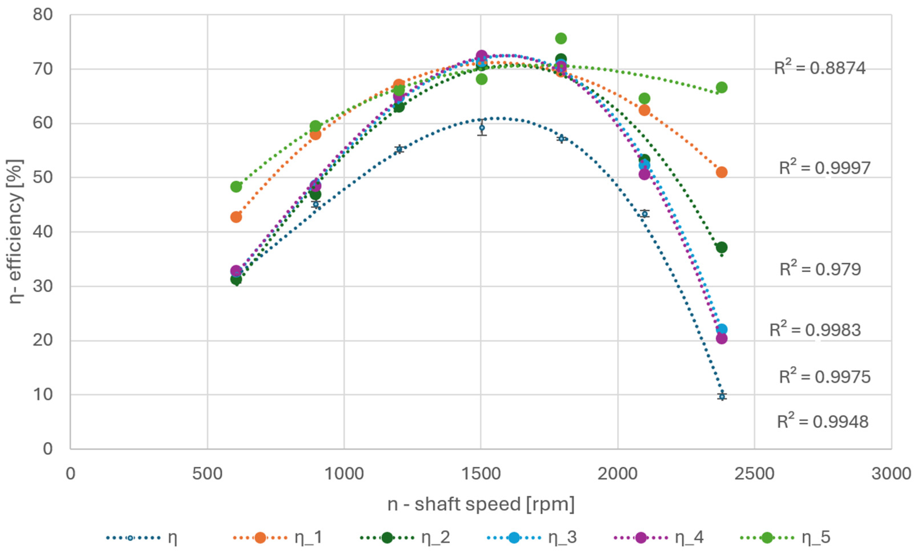
Figure 7 illustrates the total PAT efficiencies. The red curve η represents the values measured on the circuit. The curve shape in setting 1, labeled η_1 in the graph, was almost identical. Only the calculated values were approximately 10% higher than the measured values. The values in settings 2, 3, and 4, labeled η_2 to η_4 in the graph, were at lower and higher speeds, very close to the values measured on the test circuit. The difference increased up to 10% at points close to the BEP. There were major computational problems in setting 5, both in achieving convergence and settling the observed values, especially at the highest speed.

Fluid Velocity and Pressure Fields

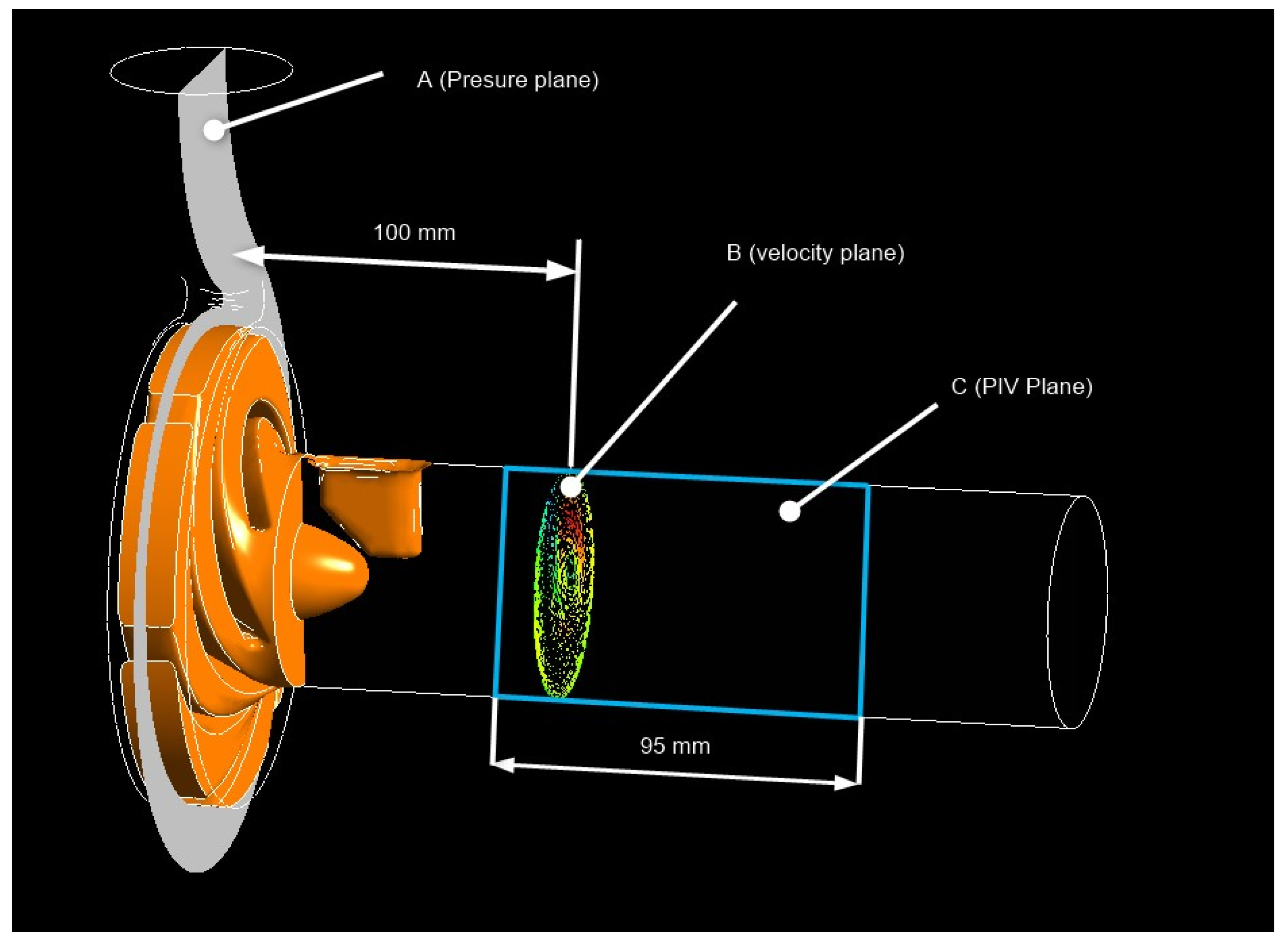
Another output of the numerical models was vector maps of fluid velocities in the PAT draft tube, which were compared with PIV measurements. Figure 8 shows the planes in which each observation was made. In the A plane, maps of the pressure fields in the spiral casing and impeller were created in the numerical model. In the B plane, which is perpendicular to the axis of the draft tube, the velocity field of the flowing fluid was created in the numerical model. The C plane, extending along the axis of the draft tube, is the plane in which the PIV measurements were performed. In the same plane, the velocity field of the flowing fluid was created in the numerical model. Subsequently, a comparison of these two outputs was performed.

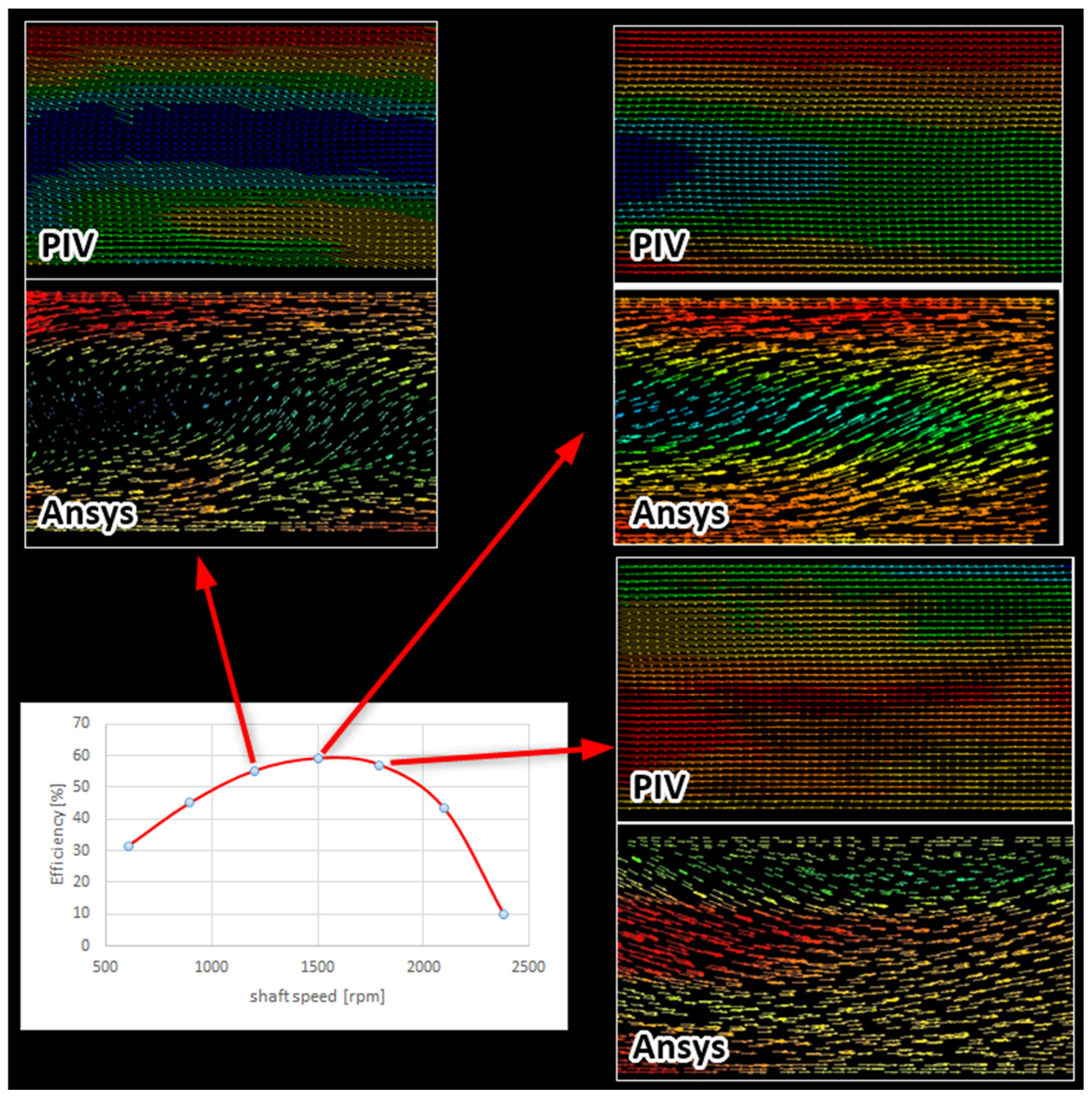
Figure 9 presents the main summary of the two outputs, PIV and Ansys, in settings 1 and 2, where the streamlines and fluid velocity distributions near the BEP best matched the PIV measurements. Similar velocities and shapes of streamlines were also obtained in settings 3 and 4. Setting 5 showed significant discrepancies in the velocities and magnitude of the outlet pressure. Therefore, the settings with the best agreement and the shortest computational times, i.e., settings 1 and 2, were further compared with the PIV measurements. For illustration, the measured output characteristic of the dependence of turbine efficiency on shaft speed is provided in the lower-left corner of Figure 9. PIV images were taken at each point and numerical simulations were performed using Ansys (https://www.ansys.com/) with the corresponding input variables. Only three comparisons of PIV vs. Ansys graphical outputs for values close to BEP are shown, for clarity.

In the figures showing the Ansys and PIV velocity fields, the liquid flows from left to right in the draft tube. The velocity vectors vary in color according to size. The highest velocities are depicted in red, the lowest in blue. The scales of the vectors vary slightly from image to image, so they are not presented in the figure for clarity.

When comparing the fluid velocity fields (1200 rpm, Figure 9, top left), a dark area can be seen running down the center of the cross section, i.e., a lower velocity in the axis of the tube than at its circumference. A similar effect can be seen at 1500 rpm when the area is wider and shifted to the left, closer to the impeller. In the third image (1800 rpm, bottom right), the PIV and Ansys both show a vortex forming at the tube axis. It has a higher velocity at the axis than at the circumference this time. This change is more pronounced in the numerical model, indicating that the turbine is outside the BEP. Therefore, the optimal vortex-free PAT operation will be between 1500 and 1800 rpm. This fact is indicated by the radial flow cross-section images produced in Ansys (see Figure 10).

Here, the radial component of the fluid velocity in the tube is clearly visible. At low shaft speed, a vortex forms close to the tube axis. As the shaft speed increases, the vortex moves off-axis and form secondary vortices. In the area of highest efficiency, the vortex reverses the direction of rotation and continues to vortex off-axis. However, a detailed comparison and accurate description of vortex formation using the PIV method would require 3D PIV measurements because the particles in the draft tube perform a general spatial motion and thus fall outside the monitored plane for 2D PIV measurements.

In addition to the above velocity fields, the fluid pressure distributions in the impeller and adjacent spiral casing were also modeled in Ansys. Figure 11 presents the pressure fields in the A plane (see Figure 9) related to all seven measured points of the efficiency course as a function of shaft speed. All images have a uniform pressure scale indicated in the figure.

A detailed view of the pressure courses in the inter-blade space at mid-blade height is presented in Figure 12. Again, all images have the same scale. The entrance to the impeller, i.e., the transition from the spiral casing to the blades, is on the left, and the exit from the impeller before the connection to the draft tube is on the right. The figures indicate that outside the optimum, there is a vacuum at the impeller outlet, which is most pronounced in the peripheral parts of the characteristic. A large pressure change can also be observed at the impeller inlet at lower speed. In the area of highest turbine efficiency, the pressure remains close to the atmospheric pressure. At higher speed, the pressure from the spiral casing to impeller transition increases and extends into a larger part of the inter-blade space.

4. Conclusions

The study focused on finding the optimal combination of input variables for PAT flow simulation in Ansys CFX. It was found that different combinations of input parameters can be used to obtain relatively accurate results.

In setting 1, where the PAT inlet pressure and PAT outlet flow were used as input variables for the simulation, the resulting efficiency had the same course, but the values were 10% higher. This setting was one of the fastest in terms of computation time.

Setting 2, where the PAT inlet flow and PAT outlet pressure were set for the simulation, had efficiency courses similar to settings 3 and 4. The calculation times were similar to setting 1.

Setting 3, where the PAT input and output pressures were set, showed a slightly longer computation time (15% on average) than setting 1. Near the BEP, the values were comparable to setting 1, i.e., the calculated values were approximately 10% higher than the measured values. The values in the peripheral parts of the characteristic differed by less than 5%.

In setting 4, where the inlet pressure was set, and the outlet pressure was set to zero, the results were almost identical to those of setting 3 in all parameters. However, its calculation time was longer, by as much as 30% in some cases.

In setting 5, the inlet velocity and outlet flow rate of the PAT were used. The calculation achieved similar values to the measured ones at low speeds, but at higher speeds above 1500 rpm, a drop of up to 100 kPa in pressure values was observed compared to the measurements. The calculation also showed convergence problems and no longer converged at all at higher speeds. While relative agreement with the measurement can be achieved in this setting, there is a greater likelihood that the program will not reach a solution. Therefore, this setting cannot be recommended.

The torque values in all simulations were significantly higher than those measured on the test circuit. This error can probably be attributed to the simplifying aspects of the simulation, which in turn will increase the overall efficiency. This is mainly due to the effect of roughness, geometry simplification (to simplify and speed up the calculation), volumetric and mechanical losses, and the type of Ansys calculation module.

Considering all the above findings and experience, the best results for numerical modeling of PAT were obtained by combining the input parameters inlet pressure and outlet flow according to setting 1. A comparison of the vector fields measured by PIV and those modeled in Ansys showed that the mathematical models could reliably produce streamlined shapes in the draft tube behind the turbine. Satisfactory agreement between the calculated and measured parameter courses thus provides a way to determine the necessary performance characteristics to optimize the pump selection for turbine operation.