Pressure Interpolation in Water Distribution Networks by Using Gaussian Processes: Application to Leak Diagnosis

Abstract

This work presents the reconstruction of the pressure head map of a water distribution system (WDS). This approach relies on historical data collected from a reduced number of sensors placed at some nodes of the WDS. Thus, a Gaussian regression process is then applied to estimate the pressure head at those nodes without a sensor, which allows the reconstruction of the pressure map for the whole network. Then, for leak diagnosis purposes, a dataset of pressure head maps of the WDN is created considering leaky scenarios, and a correlation method is applied to estimate the leak location. Then, for clarity, the Hanoi network is used to evaluate the performance of this leak diagnosis strategy in a simulation environment, assuming the availability of only three sensors. The results showed the potential for pressure head map reconstruction and leak localization.

1. Introduction

The effective management and control of a water distribution network (WDN) requires an accurate regulation of the pressure head regardless of the demand pattern. In general, it is essential to avoid low-pressure conditions that compromise the current demand-supply balance, while also preventing overpressure situations that can cause damage, such as leaks. This is particularly important because pipelines are designed to operate at full capacity under steady-state flow conditions, which increases the potential for such issues [1]. In practice, water management companies use fewer pressure sensors to monitor the pressure head along the network due to a limited budget and because it is difficult to install them, especially for underground pipelines. Therefore, the network control level is proportional to the number of monitored nodes. However, the limitation of the available sensors is a disadvantage. To face this issue, this work proposes an interpolation-based method to estimate the pressure head in those nodes without a sensor using the available pressure head measurements. Thus, it is possible to build a complete map of the pressure head along the water network that, in turn, can help apply better pressure regulation and identify leakage scenarios, even for multi-leak scenarios. Nonetheless, when building a complete map of the pressure head, two issues arise (a) sensor placement and (b) the estimation of the pressure head at nodes without sensors. Since our paper focuses on estimating pressure heads at nodes without sensors, to overcome the first problem, a well-known sensor placement procedure is used just as described in [2,3], for instance. Thus, we focus on the problem of estimating the pressure head in the nodes without sensors. Here, a regression-based interpolation method with Gaussian processes is proposed. The design of such an interpolation algorithm also implies determining other variables (hydraulic parameters) that complement the information provided by the pressure sensors, such that the estimation of unknown pressures is as accurate as possible. A limitation of such an algorithm is that in a typical network, the number of sensors is small compared to the total number of nodes, and the available measurements are usually corrupted by some noise. The accurate estimation of the unmeasured pressures in this situation represents a significant challenge. The proposed method based on Gaussian processes aims to minimize the effects of these limitations.

The estimation of the pressure head in the nodes of a WDN has already been explored using pressure head measurements only in a few nodes. In [4], the authors proposed an interpolation method known as kriging, where the pressure head in the nodes without sensors is estimated using an interpolation-based approach. This method is then applied to the leak diagnosis problem using convolutional neural networks (CNN) besides pressure head estimations. However, this method needs to be improved in adjusting the CNN design by creating a good image data set [5]. Moreover, in the case of large-scale WDN, the estimation of the pressure head is performed based on the Matrix completion approach. However, the pressure estimations lack accuracy in comparison with branched networks [6]. In [7,8], additional and different hydraulic variables of the WDN are proposed to improve these estimations’ accuracy.

On the other hand, genetic algorithms have also been applied to estimate the demand in the nodes of the WDN as an initial step without using any sensor placement strategy. In other words, the demand estimation has been performed by using a set of randomly placed sensors along the WDN with accurate results [9,10]. Moreover, in [11], Artificial Neural Networks (ANN) have been employed to estimate pressure head in non-sensed nodes in a WDN with a ±2 m error. These results were used to create a hybrid model to estimate the roughness of the pipes. Following this direction, in [12], an Iterative Hydraulic Interval State method is used to estimate flow rate and pressure head for leak diagnosis purposes. On the other hand, in [13], numerical methods such as the Gauss–Newton and Newton–Raphson methods are used to estimate the model state of a WDN. However, the computational cost is high, and the estimation needs adjustment work. A genetic algorithm-based approach is used to calibrate the WDN’s parameters accurately, which helps implement a sensor placement method for leak diagnosis purposes [14,15]. In [16], a machine learning technique is used for leak diagnosis purposes by implementing the Random Forest classifier in which the segmentation of nodes throughout the WDN is performed. Although the leak diagnosis is achieved with success, the computational cost is high, especially for multi-leak scenarios for large-scale WDN. In [17], the data-driven approach has also been used to locate leaks by implementing the clustering of the WDN with the graph theory. Such an approach estimates a new variable in a node without a sensor by using the flow direction in the shortest path. However, it requires using many nodes with a sensor, which is not feasible in practice. Other classifier methods also exist, such as K-means type clustering, in which a hydraulic model of the WDN is used. It classifies leak scenarios correctly, but it can be enhanced with an improved hydraulic model or by modeling the WDN in another way [18]. In [19,20], the support vector machine approach has been used to classify the region where a leak appears in a WDN. In this approach, the method first uses data from the sensors installed along the network. An accurate leak localization result is obtained, especially for short-scale WDN. Conversely, this is no longer true for large-scale WDN.

The CNN-classifier-based leak diagnosis approach uses a sectorizing of the WDN to locate leaks. This technique has been tested in three different WDNs with acceptable results. However, it could be improved with the use of multiple classifiers [21]. In [22] regression by Gaussian processes methods, artificial neural networks (ANN) and a hybrid method between support vector machine and grasshopper optimization and GPR are used to estimate the state of rupture in a WDN by a hydraulic and calibrated model of the WDN. It was observed that the GPR performed the best. Following this direction, GPR interpolation has also been explored for water quality analysis purposes as in [23] and applications in the medical field [24]. As mentioned above, the GPR method has efficiently estimated variables and will be used in our application.

The main contribution of this paper is the pressure estimation procedure based on Gaussian processes since it is novel and innovative because it implies, on the one hand, a lower hydraulic modeling dependence in comparison with other available approaches and, on the other hand, a good trade-off between simplicity and accuracy no matter noisy measurements, and those aspects are widely desirable in practice. Thus, it is possible to reconstruct a pressure head map for the whole WDN by using a reduced number of sensors installed along it, allowing the leaks to be identified.

The rest of the document is organized as follows: in Section 2, the pressure interpolation method is formally described and some guidelines for its implementation are given. In Section 3, the results of the proposed method applied to a simplified version of the Hanoi network (case study) are presented and discussed. Finally, Section 4 presents the conclusions and future related works are proposed.

2. Material and Methods

2.1. Foundation of Gaussian Processes

A Gaussian Process (GP) is an infinite collection of random variables satisfying the condition that a multivariable Gaussian distribution is fulfilled for any finite subset of such a collection. Moreover, Gaussian Processes are non-parameterized data models using continuous functions to quantify means and covariances. This is presented in Equation (1):

$$f\left(x\right)\sim \mathrm{GP}(m\left(x\right),k(x,x^{\prime })),$$

(1)

where $f\left(x\right)$ is used to represent the Gaussian process, x and $x^{\prime }$ are any finite set of variables taken from the full data set (infinite collection), $m\left(x\right)=E\left[f\right(x\left)\right]$ is a mean function of the available data set, and $k(x,x^{\prime })=E\left[(f\left(x\right)-m\left(x\right))(f\left(x^{\prime }\right)-m\left(x^{\prime }\right))\right]$ is a covariance function used to measure the strength of the relationship between x and $x^{\prime }$.

Assuming a set ${\left\{x_n\right\}}_{n=1}^N$ of points in ${\mathbb{R}}^D$, where D is the number of input variables (features) of any system under consideration, and $x,x^{\prime }\in {\mathbb{R}}^D$. Then, by the definition of GP given by [25], the following matrix representation can be formulated:

$${[f\left(x_1\right),f\left(x_2\right),\dots ,f\left(x_N\right)]}^{\top }\sim {\mathcal{N}}_N(\mathbf{m},\mathbf{K}),$$

(2)

where $\mathbf{m}$ is a vector such that ${\mathbf{m}}_n=m\left(x\right)$, and $\mathbf{K}$ is a matrix such that ${\mathbf{K}}_{n,m}=k(x_n,x_m)$. There is no restriction on $m\left(x\right)$, but $k(x,x^{\prime })$ must be a kernel function to ensure that $\mathbf{K}$ is a positive semidefinite and symmetric matrix. In Gaussian Processes focused on Regression (GPR), a commonly used kernel is the Radial Basis Function (RBF):

$$k(x,x^{\prime })={\theta }_1^{2}exp\left(-\frac{1}{2{\theta }_2^2}{\parallel x-x^{\prime }\parallel }^2\right),$$

(3)

where ${\theta }_1$ and ${\theta }_2$ are hyperparameters tuned on GP training.

GPs can be used as predictive models to solve regression problems. Moreover, a regression-based Gaussian process with spatial/geographical prediction of unknown variables is known as kriging. When time is involved as a new variable (for dynamic systems), the GP leads to Kalman filtering [26,27]. Furthermore, GP regression is not limited to spatial or temporal variables since it can be used with any type of predictor variable, even those that do not have a physical meaning. In regression applications, in addition to the input variable x, a response variable y determined by the Gaussian process $f\left(x\right)$ is assumed as:

$$y=f\left(x\right)+\epsilon ,$$

(4)

where $f\left(x\right)\sim \mathrm{GP}(m\left(x\right),k(x,x^{\prime }))$, and $\epsilon \sim \mathcal{N}\left(0,{\sigma }_n^2\right)$ is a Gaussian noise. In practice, $m\left(x\right)$ is not known and is estimated from the data by assuming that

$$\begin{array}{cc}\hfill f\left(x\right)& =g\left(x\right)+\mathbf{h}{\left(x\right)}^{\top }\beta ,\hfill \end{array}$$

(5)

$$\begin{array}{cc}\hfill g\left(x\right)& \sim \mathrm{GP}(0,k(x,x^{\prime })),\hfill \end{array}$$

(6)

where $\mathbf{h}\left(·\right)$ is a basis function (e.g., polynomial), and the parameter $\beta$ is optimized together with the hyperparameters of the covariance function. The most common methods to optimize GPs are the well-known cross-validation and the Bayesian model selection, which can be performed just as described in [25]. The optimization of such hyperparameters helps to obtain a better estimation.

2.2. Pressure Interpolation Using GPR

Water distribution networks are often equipped with sensors to measure variables like pressure head and flow rate. However, sensors are often installed in only a few nodes for economic reasons. Pressure head measurements are used for leak isolation purposes since the difference in pressure between a leaky scenario and non-leaking conditions is assumed. In this way, the Gaussian Process Regression approach, as described in Section 2.1, is used to estimate the pressure head at nodes without sensors using an interpolation procedure and the available pressure head measurements. To accomplish this, the proposed GPR uses as variables for prediction of the total hydraulic head (H) coming from nodes with sensors $S_1,S_2,\dots ,S_N$ and the shortest path lengths from all nodes without sensors (node n) towards those having sensors. Therefore, the GPR represents a mapping such that:

$$\varphi :{\mathbb{R}}^{2N+1}\to \mathbb{R}.$$

(7)

This allows us to estimate (via interpolation) the pressure head at the nodes without sensors. This can be expressed as follows:

$${\widehat{H}}_n=\varphi (H_{S_1},H_{S_2},H_{S_N}\dots ,L_1,L_2,\dots ,L_N,L_R),$$

(8)

where ${\widehat{H}}_n$ is the estimated hydraulic head at node n, $H_{S_i}$ is the hydraulic head measured by the i-th sensor, $L_i$ is the length of the shortest path from node n to the i-th node with the sensor, and $L_R$ is the length of the path traveled by the water from the reservoir to node n. A scheme summarizing the relationship between the predictor and response variables is shown in Figure 1.

Although the pressure heads measured by sensors ($H_{S_i}$) seem to be the most relevant predictor variables to estimate the pressure at nodes without sensors, the separating length between the interpolated node and the nodes with sensor ($L_i$) also helps to determine the relevance of each measured pressure. The length traveled by the water from the reservoir ($L_R$) is also useful as a predictor variable since the pressure at each node is assumed to be the reservoir pressure decreased by an amount related to this length. Figure 2 shows a hypothetical case where the hydraulic head at a node (n) can be estimated from the measurements provided by three pressure sensors (associated with $H_{S_1}$, $H_{S_2}$ and $H_{S_3}$). The pipeline lengths ($L_1$, $L_2$, and $L_3$) are computed by adding the lengths of the pipes connecting the interpolated node to the sensed nodes along the shortest path (e.g., $L_2=L_{2,1}+L_{2,2}+L_{2,3}$).

Remark 1.

The lengths $L_i$ for each target node n are precomputed and stored in a constant matrix since they do not change throughout the process. Instead, the length $L_R$ must be calculated dynamically on each new interpolation since the water can flow through a different path when leaks and when the network is supplied by multiple tanks whose water levels change differently throughout the day.

In the mini-network shown in Figure 2, the shortest path between any pair of nodes can be determined by inspection, but in large-scale networks, finding the shortest path takes work. However, this is a problem that has been solved in graph theory. Some methods for computing shortest path lengths (Bellman–Ford and Dijkstra algorithms) are described in [28], and optimized versions can be found in [29]. A basic version of Dijkstra’s algorithm is used in this work.

2.3. Leak Localization

A correlation-based technique is used for solving the single leak problem as reported in [30,31]. This technique uses the whole pressure head map obtained through the GPR algorithm, i.e., $\widehat{\mathbf{H}}=[{\widehat{H}}_1,{\widehat{H}}_2,\dots ,{\widehat{H}}_n]$ where n is the number of nodes in the WDN. A classification tree is used to apply the correlation technique; a detailed description of the tree classification and its optimization methods can be found in [32,33,34]. To apply the correlation technique, a training stage is first performed as follows: several experiments are performed considering the occurrence of leaks at all nodes of the WDN as follows: for the i-th node $i=1,2,\dots ,\kappa$ a set of leak magnitudes $j=1,2,\dots ,\gamma$ are simulated, that is, a set of $\kappa \times \gamma$ different leak scenarios are simulated and recorded. Once this set of experiments is saved, 80% of them are used for training, and the remaining 20% is used for testing.

Algorithm 1 provides the general framework used to address the problem of leak localization using both machine learning techniques, the Gaussian process and decision tree classification.

Algorithm 1: Water Leak Localization in a Distribution Network
Part	1: Pressure Estimation Using Gaussian Process Regression
	Inputs: Pressure measurements at specific instrumented nodes, and pipe lengths. Outputs: Estimated pressures at all nodes.
	Initialize Gaussian Process Regression (GPR) with a suitable kernel function, e.g., Radial Basis Function (RBF). Set the input features as the measured and non-measured node pressures and lengths of connecting pipelines. Set the target output as the non-measured node pressures. Train the GPR model using the available data: (a) Optimize the hyperparameters of the kernel based on the data. (b) Fit the GPR to the input features and target outputs. Predict pressures at all nodes (both measured and unmeasured) using the trained GPR model. Store the estimated pressures for each node.
Part	2: Leak Localization Using Decision Tree Classification
	Inputs: Estimated node pressures from Part 1. Outputs: Probable locations of leaks.
	Define the features for classification: Estimated pressures in all nodes. Label data based on historical or simulated leak information: Data instances corresponding to leaks at the n-th node are labeled as “Class n”. Initialize a decision tree classifier. Train the decision tree using the labeled dataset: Split the data into training and test sets. Fit the decision tree to the training data. Optimize tree hyperparameters like depth and minimum samples per leaf. Use the trained decision tree to classify all nodes: Predict the most likely node where the leak is located based on its features. Output the node that is predicted to leak along with its leak probability.

3. Results

To evaluate the performance of the GPR-based interpolation approach in solving the leak diagnosis problem, the well-known Hanoi network (see Figure 3) is used [35,36]. This network consists of 32 nodes (31 junction nodes and one reservoir) and 34 pipelines with a total length of 39,420 m.

After the sensor placement process was performed using the procedure reported in [2,3], nodes 12, 21, and 27 are considered to have pressure head transducers installed. Thus, ${\mathbf{H}}_S={\left[H_{S_1}{H}_{S_2}{H}_{S_3}\right]}^{\top }={\left[H_{12}{H}_{21}{H}_{27}\right]}^{\top }$. Then, a simulation was performed assuming a leak-free scenario using the EPANET-MATLAB Toolkit [37,38] by considering the base demands shown in Figure 4. Then, considering that there are $\kappa =31$ nodes and that for each node $\gamma =50$ different leak magnitudes were simulated, that is, $Q_{\mathrm{leak}}=\{1,2,\dots ,50\} \mathrm{L}/\mathrm{s}$, a total of 1550 leak scenarios were simulated and recorded. The time duration of both kinds of simulations, namely, leak-free and leaky scenarios, is 24 $\mathrm{h}$ with a sampling rate of 1 $\mathrm{h}$, starting at 00:00 (midnight). In all leak scenarios, the leak was considered to occur at 2:00 a.m. and kept active until the end of the simulation.

In order to select the optimal combination of nodes where to place the pressure sensors, two different methods were used: The first is based on information theory, which maximizes the relevance of the information provided by the set of sensors about the location of the leaks while minimizing the redundancy of the information provided by each sensor [3]. The second is based on the simulated annealing metaheuristic, which seeks the combination of nodes that minimizes the percentage of error in locating leaks from the measurements provided by sensors placed on those nodes [2]. In the Hanoi network, both methods led to the same sensor placement, which is the aforementioned: nodes 12, 21, and 27.

To determine the number of pressure sensors to use, a marginal analysis was carried out. This procedure consists of progressively increasing the number of sensors until adding a new sensor does not provide a significant benefit from a statistical approach, as described in [3].

To train the GPR algorithm, both the hydraulic head at nodes with a sensor: ${\mathbf{H}}_S={[H_{12},H_{21},H_{27}]}^{\top }$ and the pipeline lengths $L_i$ (along the shortest path) from the i-th node to each sensed node (including the reservoir) ${\mathbf{H}}_S$ (see Figure 5) are required and are considered as the input and the output is the estimated pressure head at $H_n$, see Figure 1. Since GPR training is performed based on a supervised learning method, a data set of the Hanoi WDN is used. The available data were separated into two sets: 80% was randomly selected for the training stage while 20% was selected for the testing stage using the MATLAB Statistics and Machine Learning Toolbox. [39]. After testing several approaches of the kernel, the Rational Quadratic type Kernel [25,40] was demonstrated to be the best option for the application. Figure 6 shows the result of interpolating the pressure head along the Hanoi WDN.

It should be noted that besides the pressure head at $H_n$ the pressure head along the pipeline path is also estimated. This fact highlights that leaks between nodes could also be localized, which is very interesting in practice. For a better interpretation of the results, in Figure 6, a heatmap representation of the pressure head interpolation is shown. It should be noted that in Figure 6, the pressure head map of the Hanoi WDN corresponds to a nominal operation, i.e., operation in a free-leak condition.

Locating leaks at intermediate locations in the pipes, not only at the nodes, can be implemented in two different ways: The first way consists of defining “virtual nodes” along the pipe and associating new classes to them in the classifier (new leaves on the classification tree). However, it should be noted that the precision in locating the leak in this case will be determined by the granularity or separation of the virtual nodes. The second way is to apply a leak location method for single pipes, such as that described by [41], since the pressures at the end nodes are already known from GPR. However, none of these extensions of the proposed methodology are explored in depth in this article.

3.1. Examples of Leak Isolation under Noise-Free Conditions

Estimating pressure heads at nodes without sensors can be used to build the whole pressure head map, which is helpful for several purposes. On the one hand, to guarantee the compliance of pressure service to the consumers, and on the other hand, for leak diagnosis purposes, among others. If a leak occurs, the pressure map could help identify the leaky candidate node by using both a pressure head map in a leak-free condition and a pressure head map in a leaky condition. A comparison of both maps will show the most significant difference at the leaky node.

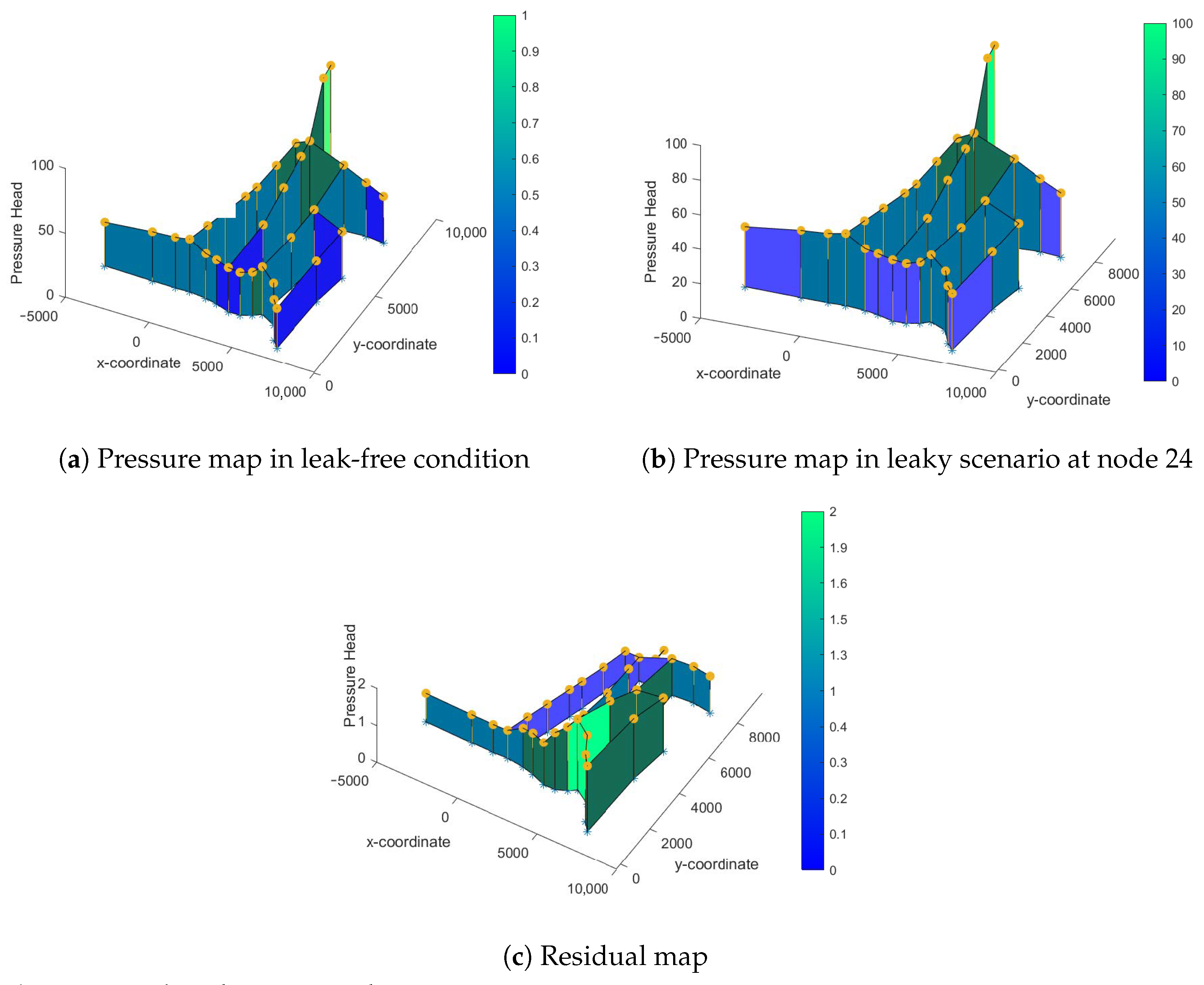
3.1.1. Case 1: Leak at Node 24

In this case, a leak is induced at node 24 at 2:00 a.m., and it is kept active until 24:00 h. The pressure head map under this leaky condition is built by using the GPR method. Then, this leaky map is compared with the leak-free map, and the residual between them is generated. In Figure 7a, the pressure head map in a leak-free condition is shown, whereas the leaky pressure head map is presented in Figure 7b. Finally, in Figure 7c, the residual between both scenarios is depicted. As can be seen, the most significant residual corresponds to node 24.

Table 1. Changes in residuals and pressures at different moments of the hour in node 24.

Hour	Candidate Node	Pressure	Residual
4:00	24	38.7372	1.9205
8:00	24	38.8332	2.0165
12:00	24	38.8271	2.0104
16:00	24	38.7944	1.9777
20:00	24	38.8301	2.0134
24:00	24	38.8598	2.0431

shows the pressure residual at node 24 computed from the pressure estimated by GPR when the leak occurs at that node.

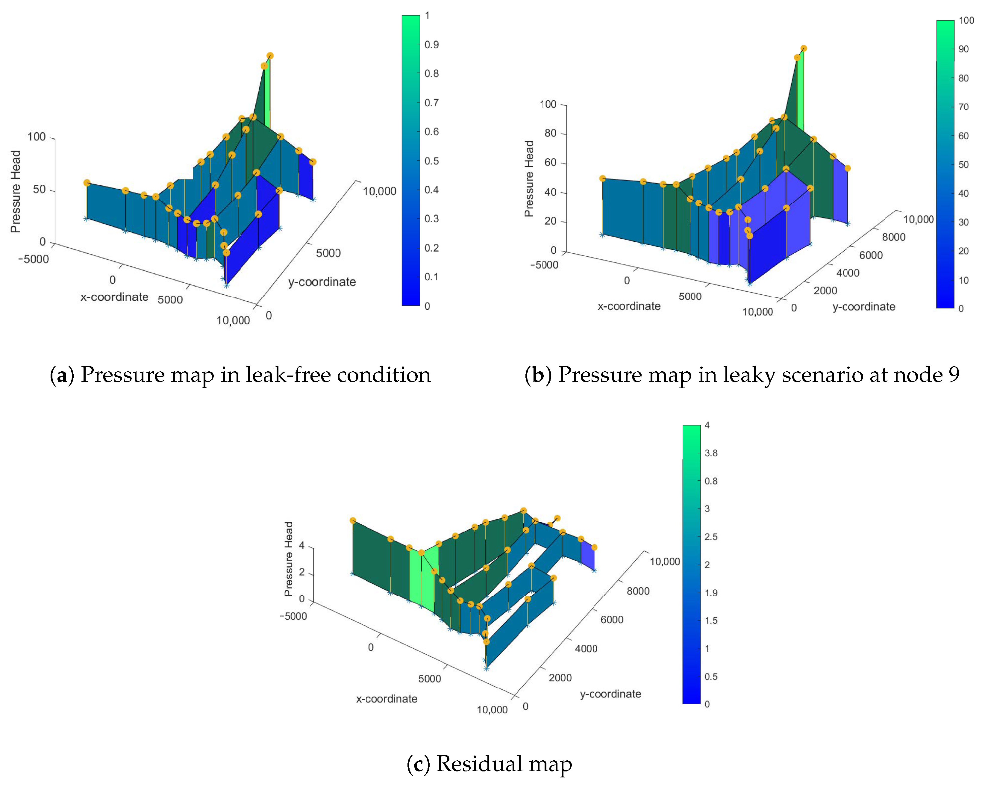
3.1.2. Case 2: Leak at Node 9

In the second case, a leak is induced at node 9 at 2:00 a.m., and it is kept active until 24:00 h. The pressure head map under this leaky condition is built by using the GPR method. Then, this leaky map is compared with the leak-free map, and the residual between them is generated. In Figure 8a, the pressure head map in a leak-free condition is shown, whereas the leaky pressure head map is presented in Figure 8b. Finally, in Figure 8c, the residual between both scenarios is depicted. As can be seen, the most significant residual corresponds to node 9.

Table 2. Changes in residuals and pressures at different times in node 9.

Hour	Candidate Node	Pressure	Residual
4:00	9	45.0551	3.9741
8:00	9	45.0409	3.9599
12:00	9	44.8347	3.7537
16:00	9	44.9123	3.8313
20:00	9	45.0352	3.9542
24:00	9	44.1563	3.0753

shows the pressure residual at node 9 computed from the pressure estimated by GPR when the leak occurs at that node.

From the data set created from the pressure maps, Gaussian white noise is added to the pressure recorded at nodes with sensors. In Figure 9, the effect of signal-to-noise ratio (SNR) ranging from 20 dB to 100 dB in the RMSE of the prediction error is presented. This figure shows that for SNR greater than 40 dB, a low prediction error (less than 0.12 m) is obtained when interpolating the unmeasured pressure heads, and it does not vary significantly above 50 dB. This means that the pressure estimation by GPR is robust enough to measure noise under typical operating conditions in real distribution networks.

3.2. Examples of Leak Diagnosis by Using the Classification Tree Algorithm

For the leak location method using the classification tree, the model was trained with the pressure maps obtained from the pressure interpolation of the Hanoi network (see Figure 3), in which 32 labels are created. The first 31 labels correspond to the 31 nodes of the WDN (excluding the reservoir), and an extra label (“0”) was created for the leak-free condition. For the test of the algorithm, a demand of 30 L/s was increased in different nodes, obtaining the pressure maps under that condition. The algorithm was tested as shown in Figure 10 and Figure 11, correctly identifying the leaking node. This same test was performed for all nodes in the network.

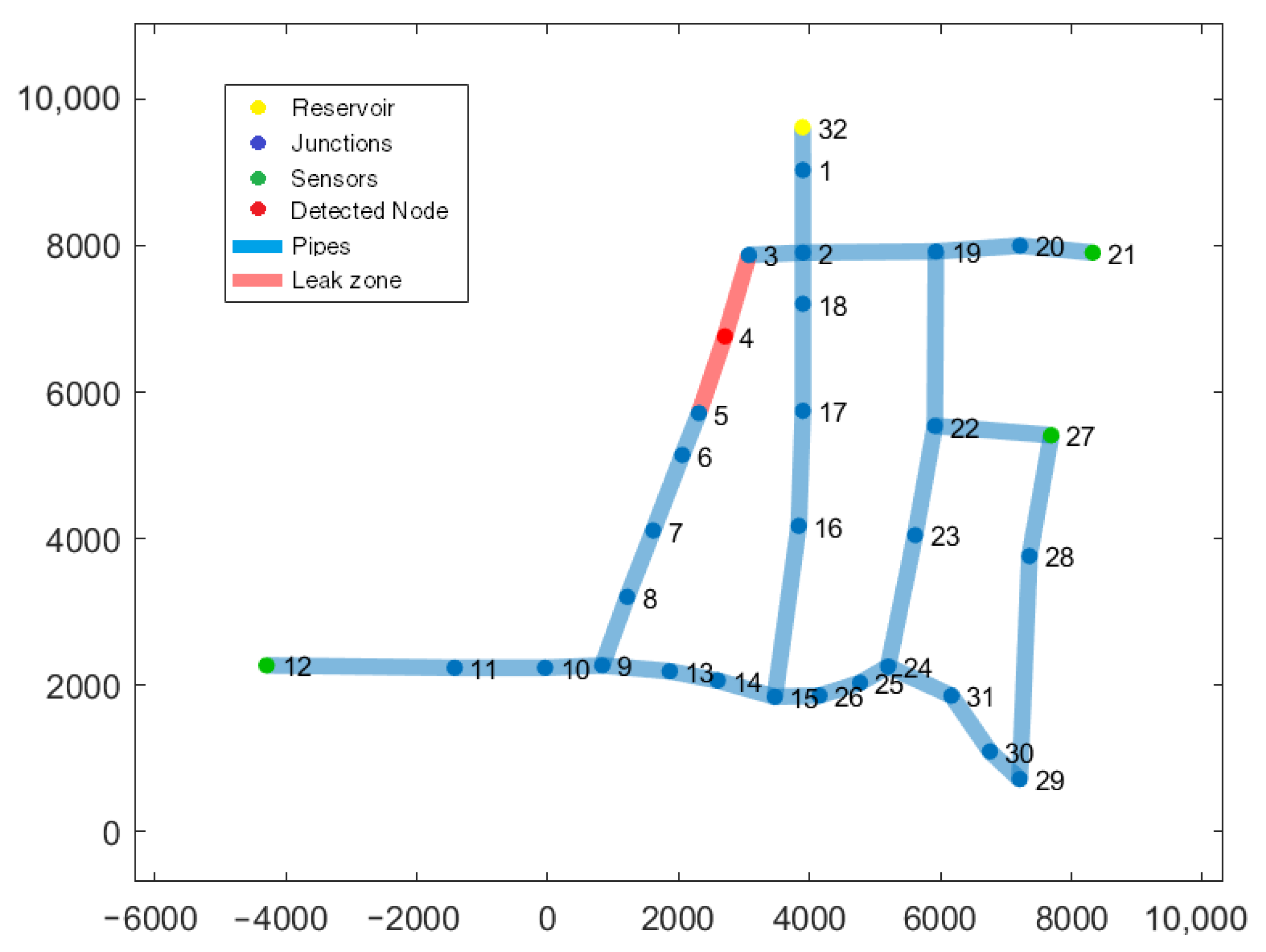
3.2.1. Case 1: Leak at Node 4

A leak is simulated at node 4 (see Figure 3). The GPR algorithm estimates the pressure head in the nodes without a sensor. Then, it is possible to reconstruct a pressure head map of the whole network using both the pressure head measurements and the estimations provided by the GPR algorithm. The classification tree algorithm processes the pressure head map and provides an estimation of the leaky node. In Figure 10, the red node represents the leaky node, and the pipes connected to it are also marked in red. In this case, the leaky node is correctly identified.

Figure 10. Hanoi network; leak case at node 4.

Figure 10. Hanoi network; leak case at node 4.

3.2.2. Case 2: Leak at Node 13

In this case, a leak is induced at node 13. In the same way as before, the whole network’s pressure head map is obtained using the GPR algorithm and the available measurements. In Figure 11, the leaky node is correctly identified (red node).

Figure 11. Hanoi network; leak case at node 13.

Figure 11. Hanoi network; leak case at node 13.

3.3. Discussion of the Results

The GPR interpolation process has been successfully applied to reconstruct Hanoi’s network’s whole pressure head map. With it, it has been possible to identify all possible leak scenarios correctly. It should be noted that during the testing process with 20% of the dataset data, the algorithm provides an estimation error of 2%. On the other hand, the classification tree algorithm was compared with the k-NN classification algorithm. As shown in

Table 3. Classification error comparison between k-NN and tree classifiers.

Classification Method	Classification Loss
k-NN with 50 neighbours, using cosine distance	0.9280
k-NN with 50 neighbours, using correlation distance	0.7066
Classification tree with default hyperparameters	0.1967
Classification tree with optimized hyperparameters	0.0260

, the classification tree algorithm performed better than the classification by k-NN.

Table 4. Comparison of classification between the pressure map of all the nodes of the network and using classification using only three sensors of the network.

SNR (dB)	Using 3 Sensors	Sensing All Nodes
40	0.9067	0.0253
45	0.8540	0.0253
50	0.7427	0.0280
55	0.6300	0.0273
60	0.4820	0.0273
∞	0.1920	0.0267

compares two leak location methods: the classification trees approach, and the k-NN-based method presented by [31]. The results evidenced a better performance when applying classification trees.

The sensitivity of the interpolation method was analyzed by introducing small perturbations into the pressure data (i.e., synthetic noise), and observing how these variations affect the interpolation results. For perturbations of the order of 1/100 of the true pressures, the error in the interpolated pressure heads remained below 0.12 m which is comparable to the uncertainty when measuring pressures instead of interpolating them.

In addition, cross-validation testing was used by dividing the data into training and test sets to measure the accuracy of interpolation in different partitions of the data. The results show that the method is robust, maintaining a low variability in the interpolation in the face of changes in the input data when evaluating the interpolation errors using the MSE metric.

It should also be noted that to obtain the synthetic data, different leakage and user demand scenarios were simulated to observe how the method behaves under different operating conditions. Overall, the results indicate that the proposed interpolation method is sensitive but stable.

The proposed methodology that combines pressure interpolation with leak localization by classification was tested only with synthetic data obtained through simulation. Verification with physical measurement data is an aspect that will be addressed in future work. To obtain real field data, it has been considered to build a monitoring system for the water distribution network. This system will consist of stations located at fixed positions that will capture measurements from in-situ pressure sensors and send them to a cloud computing system. The cloud system will process these data to interpolate the unmeasured pressures and then apply the leak detection and localization algorithm.

4. Conclusions

The GPR-interpolation-based approach allowed the whole pressure head map of Hanoi’s network to be accurately reconstructed under different conditions. The introduction of the water path variable made the estimation error reduction possible. With these accurate pressure head maps, the leak diagnosis problem has been successfully addressed for all possible single leak scenarios (all nodes of the network). Finally, the information on the flow direction allows the GPR-based interpolation method to be more robust. This fact is important, especially for large-scale networks where the irregular relief can change the flow direction. A more in-depth analysis of this fact will be part of future developments.

References

1. Reda, A.; Mahmoud, R.M.A.; Shahin, M.A.; Amaechi, C.V.; Sultan, I.A. Roadmap for Recommended Guidelines of Leak Detection of Subsea Pipelines. J. Mar. Sci. Eng. 2024, 12, 675. [Google Scholar] [CrossRef]
2. Morales-González, I.; Santos-Ruiz, I.; López-Estrada, F.; Puig, V. Pressure Sensor Placement for Leak Localization Using Simulated Annealing with Hyperparameter Optimization. In Proceedings of the 2021 5th International Conference on Control and Fault-Tolerant Systems (SysTol), Saint-Raphael, France, 9 November 2021; pp. 205–210. [Google Scholar] [CrossRef]
3. Santos-Ruiz, I.; López-Estrada, F.R.; Puig, V.; Valencia-Palomo, G.; Hernández, H.R. Pressure Sensor Placement for Leak Localization in Water Distribution Networks Using Information Theory. Sensors 2022, 22, 443. [Google Scholar] [CrossRef]
4. Soldevila, A.; Jensen, T.N.; Blesa, J.; Tornil-Sin, S.; Femandez-Canti, R.; Puig, V. Leak localization in water distribution networks using a kriging data-based approach. In Proceedings of the 2018 IEEE Conference on Control Technology and Applications (CCTA), Copenhagen, Denmark, 21–24 August 2018; pp. 577–582. [Google Scholar]
5. Javadiha, M.; Blesa, J.; Soldevila, A.; Puig, V. Leak localization in water distribution networks using deep learning. In Proceedings of the 2019 6th International Conference on Control, Decision and Information Technologies (CoDIT), Paris, France, 23–26 April 2019; pp. 1426–1431. [Google Scholar]
6. Mankad, J.; Natarajan, B.; Srinivasan, B. Integrated approach for optimal sensor placement and state estimation: A case study on water distribution networks. ISA Trans. 2021, 123, 272–285. [Google Scholar] [CrossRef]
7. Wang, S.; Taha, A.F.; Gatsis, N.; Sela, L.; Giacomoni, M.H. Probabilistic state estimation in water networks. IEEE Trans. Control. Syst. Technol. 2021, 30, 507–519. [Google Scholar] [CrossRef]
8. Fusco, F.; Arandia, E. State estimation for water distribution networks in the presence of control devices with switching behavior. Procedia Eng. 2017, 186, 592–600. [Google Scholar] [CrossRef]
9. Do, N.C.; Simpson, A.R.; Deuerlein, J.W.; Piller, O. Calibration of water demand multipliers in water distribution systems using genetic algorithms. J. Water Resour. Plan. Manag. 2016, 142, 04016044. [Google Scholar] [CrossRef]
10. Do, N.; Simpson, A.; Deuerlein, J.; Piller, O. Demand estimation in water distribution systems: Solving underdetermined problems using genetic algorithms. Procedia Eng. 2017, 186, 193–201. [Google Scholar] [CrossRef]
11. Meirelles, G.; Manzi, D.; Brentan, B.; Goulart, T.; Luvizotto, E. Calibration model for water distribution network using pressures estimated by artificial neural networks. Water Resour. Manag. 2017, 31, 4339–4351. [Google Scholar] [CrossRef]
12. Vrachimis, S.G.; Timotheou, S.; Eliades, D.G.; Polycarpou, M.M. Interval State Estimation of Hydraulics in Water Distribution Networks. In Proceedings of the 2018 European Control Conference (ECC), Limassol, Cyprus, 12–15 June 2018; pp. 2641–2646. [Google Scholar]
13. Tshehla, K.S.; Hamam, Y.; Abu-Mahfouz, A.M. State estimation in water distribution network: A review. In Proceedings of the 2017 IEEE 15th International Conference on Industrial Informatics (INDIN), Emden, Germany, 24–26 July 2017; pp. 1247–1252. [Google Scholar]
14. Zanfei, A.; Menapace, A.; Santopietro, S.; Righetti, M. Calibration procedure for water distribution systems: Comparison among hydraulic models. Water 2020, 12, 1421. [Google Scholar] [CrossRef]
15. Nicolini, M.; Falcomer, L. Genetic Algorithm for Calibration and Leakage Identification in Water Distribution System. In Proceedings of the 2020 3rd IEEE International Conference on Knowledge Innovation and Invention (ICKII), Kaohsiung, Taiwan, 21–23 August 2020; pp. 273–276. [Google Scholar]
16. Lučin, I.; Čarija, Z.; Družeta, S.; Lučin, B. Detailed Leak Localization in Water Distribution Networks Using Random Forest Classifier and Pipe Segmentation. IEEE Access 2021, 9, 155113–155122. [Google Scholar] [CrossRef]
17. Alves, D.; Blesa, J.; Duviella, E.; Rajaoarisoa, L. Robust Data-Driven Leak Localization in Water Distribution Networks Using Pressure Measurements and Topological Information. Sensors 2021, 21, 7551. [Google Scholar] [CrossRef]
18. Predescu, A.; Mocanu, M.; Lupu, C. A modern approach for leak detection in water distribution systems. In Proceedings of the 2018 22nd International Conference on System Theory, Control and Computing (ICSTCC), Sinaia, Romania, 10–12 October 2018; pp. 486–491. [Google Scholar] [CrossRef]
19. Liu, Y.; Ma, X.; Li, Y.; Tie, Y.; Zhang, Y.; Gao, J. Water Pipeline Leakage Detection Based on Machine Learning and Wireless Sensor Networks. Sensors 2019, 19, 5086. [Google Scholar] [CrossRef]
20. Ramotsoela, D.T.; Hancke, G.P.; Abu-Mahfouz, A.M. Attack detection in water distribution systems using machine learning. Hum.-Centric Comput. Inf. Sci. 2019, 9, 13. [Google Scholar] [CrossRef]
21. Fuentes, V.C.; Pedrasa, J.R.I. Leak detection in water distribution networks via pressure analysis using a machine learning ensemble. In Proceedings of the International Conference on Society with Future: Smart and Liveable Cities, Braga, Portugal, 4–6 December 2019; Springer: Berlin/Heidelberg, Germany, 2019; pp. 31–44. [Google Scholar]
22. Alizadeh, Z.; Yazdi, J.; Mohammadiun, S.; Hewage, K.; Sadiq, R. Evaluation of data driven models for pipe burst prediction in urban water distribution systems. Urban Water J. 2019, 16, 136–145. [Google Scholar] [CrossRef]
23. Pasolli, L.; Melgani, F.; Blanzieri, E. Gaussian process regression for estimating chlorophyll concentration in subsurface waters from remote sensing data. IEEE Geosci. Remote Sens. Lett. 2010, 7, 464–468. [Google Scholar] [CrossRef]
24. Alghamdi, A.S.; Polat, K.; Alghoson, A.; Alshdadi, A.A.; Abd El-Latif, A.A. Gaussian process regression (GPR) based non-invasive continuous blood pressure prediction method from cuff oscillometric signals. Appl. Acoust. 2020, 164, 107256. [Google Scholar] [CrossRef]
25. Rasmussen, C.E.; Williams, C.K. Gaussian Processes for Machine Learning (Adaptive Computation and Machine Learning); MIT Press: Cambridge, MA, USA, 2005. [Google Scholar]
26. Lio, W.H.; Li, A.; Meng, F. Real-time rotor effective wind speed estimation using Gaussian process regression and Kalman filtering. Renew. Energy 2021, 169, 670–686. [Google Scholar] [CrossRef]
27. Santos-Ruiz, I.; López-Estrada, F.R.; Puig, V.; Blesa, J. Estimation of Node Pressures in Water Distribution Networks by Gaussian Process Regression. In Proceedings of the 2019 4th Conference on Control and Fault Tolerant Systems (SysTol), Casablanca, Morocco, 18–20 September 2019; pp. 50–55. [Google Scholar] [CrossRef]
28. Cormen, T.H.; Leiserson, C.E.; Rivest, R.L.; Stein, C. Introduction to Algorithms; MIT Press: Cambridge, MA, USA, 2009. [Google Scholar]
29. Yuan, H.; Hu, J.; Song, Y.; Li, Y.; Du, J. A new exact algorithm for the shortest path problem: An optimized shortest distance matrix. Comput. Ind. Eng. 2021, 158, 107407. [Google Scholar] [CrossRef]
30. Bort, C.G.; Righetti, M.; Bertola, P. Methodology for leakage isolation using pressure sensitivity and correlation analysis in water distribution systems. Procedia Eng. 2014, 89, 1561–1568. [Google Scholar] [CrossRef]
31. Santos-Ruiz, I.; Blesa, J.; Puig, V.; López-Estrada, F. Leak localization in water distribution networks using classifiers with cosenoidal features. IFAC-PapersOnLine 2020, 53, 16697–16702. [Google Scholar] [CrossRef]
32. Loh, W.Y. Regression tress with unbiased variable selection and interaction detection. Stat. Sin. 2002, 12, 361–386. [Google Scholar]
33. Coppersmith, D.; Hong, S.J.; Hosking, J.R. Partitioning nominal attributes in decision trees. Data Min. Knowl. Discov. 1999, 3, 197–217. [Google Scholar] [CrossRef]
34. Breiman, L.; Friedman, J.H.; Olshen, R.A.; Stone, C.J. Classification and Regression Trees; Routledge: London, UK, 2017. [Google Scholar]
35. Savic, D.A.; Walters, G.A. Genetic algorithms for least-cost design of water distribution networks. J. Water Resour. Plan. Manag. 1997, 123, 67–77. [Google Scholar] [CrossRef]
36. Ayad, A.; Khalifa, A.; Fawy, M.; Moawad, A. An integrated approach for non-revenue water reduction in water distribution networks based on field activities, optimisation, and GIS applications. Ain Shams Eng. J. 2021, 12, 3509–3520. [Google Scholar] [CrossRef]
37. Eliades, D.G.; Kyriakou, M.; Vrachimis, S.; Polycarpou, M.M. EPANET-MATLAB Toolkit: An Open-Source Software for Interfacing EPANET with MATLAB. In Proceedings of the 14th International Conference on Computing and Control for the Water Industry (CCWI), Amsterdam, The Netherlands, 7–9 November 2016; p. 8. [Google Scholar] [CrossRef]
38. Rossman, L.A. EPANET Users Manual; U.S. Environmental Protection Agency: Cincinnati, OH, USA, 1994.
39. Paluszek, M.; Thomas, S. MATLAB Machine Learning Toolboxes. In Practical MATLAB Deep Learning; Springer: Berlin/Heidelberg, Germany, 2020; pp. 25–41. [Google Scholar]
40. Liu, M.; Chowdhary, G.; Da Silva, B.C.; Liu, S.Y.; How, J.P. Gaussian processes for learning and control: A tutorial with examples. IEEE Control Syst. Mag. 2018, 38, 53–86. [Google Scholar] [CrossRef]
41. Santos-Ruiz, I.; Bermúdez, J.; López-Estrada, F.; Puig, V.; Torres, L.; Delgado-Aguiñaga, J. Online leak diagnosis in pipelines using an EKF-based and steady-state mixed approach. Control Eng. Pract. 2018, 81, 55–64. [Google Scholar] [CrossRef]
Figure 1. Pressure interpolation scheme.
Processes 12 01147 g001
Figure 2. Three sensors monitor Response and predictor variables in a network.
Processes 12 01147 g002
Figure 3. Hanoi network.
Processes 12 01147 g003
Figure 4. Base demand in Hanoi network.
Processes 12 01147 g004
Figure 5. Shortest paths from node 15 to sensors and flow path from reservoir.
Processes 12 01147 g005
Figure 6. Interpolated pressure map: leak-free condition.
Processes 12 01147 g006
Figure 7. Leak isolation in node 24.
Processes 12 01147 g007
Figure 8. Leak isolation in node 9.
Processes 12 01147 g008
Figure 9. Variation of pressure prediction error with signal-to-noise ratio.
Processes 12 01147 g009