
A Temperature Control Method of Lysozyme Fermentation Based on LRWOA-LSTM-PID


Abstract
1. Introduction
- (1)
- A temperature mechanism model based on a dynamic equation is designed, which can better reflect the temperature changes in the fermenter.
- (2)
- A Whale Optimization Algorithm based on the Lévy flight and random walk strategy is proposed. By introducing Levy flight and random walk strategies into the Whale Optimization Algorithm, the global and local optimization abilities of the algorithm are improved. It overcomes the problem of the original algorithm falling into local extrema prematurely when dealing with complex issues.
- (3)
- A PID parameter tuning method based on LSTM is proposed. This method has the ability to learn time sequences information and capture the trend of error sequences under continuous time sampling, so the network weight can be adjusted more reasonably. As a result, it achieves the rapid tuning of the PID parameters Kp, Ki, and Kd.
- (4)
- An LSTM parameter initialization method based on the LRWOA algorithm is proposed. The method takes advantage of the excellent optimization capability of the LRWOA algorithm, overcoming the problem of traditional random parameter initialization methods falling into local optimum solutions prematurely, thereby enhancing the stability of the initial parameters of the LSTM neural network.
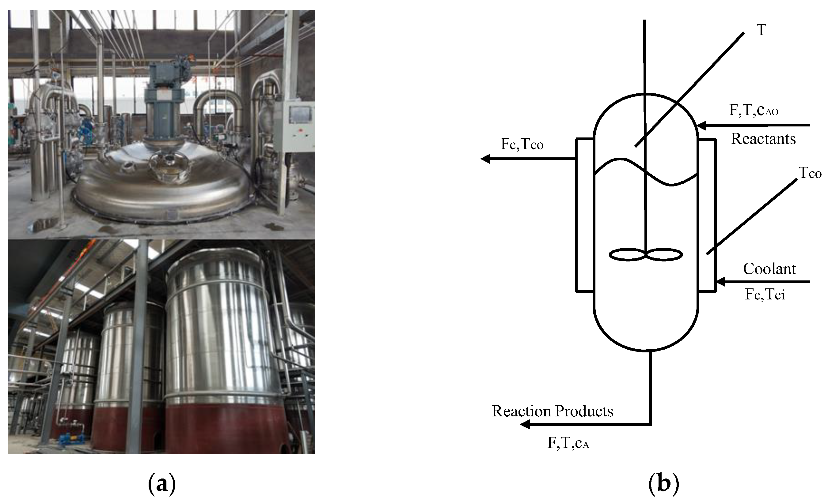
2. Modeling of Fermenter Temperature
Fermenter Temperature Mathematical Model
- (1)
- Chemical reaction rate equation
- (2)
- Material balance equation
- (3)
- The heat balance equation
3. Algorithm
3.1. Whale Optimization Algorithm
- (1)
- Encircling Prey
- (2)
- Bubble-net attacking
- Contraction enveloping mechanism: This method is roughly the same as enveloping prey, the difference being that the original range of a is adjusted from 2 to 0 to a fixed value of 1. Since a determines the range of A, the range of A changes from the original [−a, a] to now [−1, 1]. At this time, the new position of the whale individual can appear at any position between the original position and the optimal solution position.
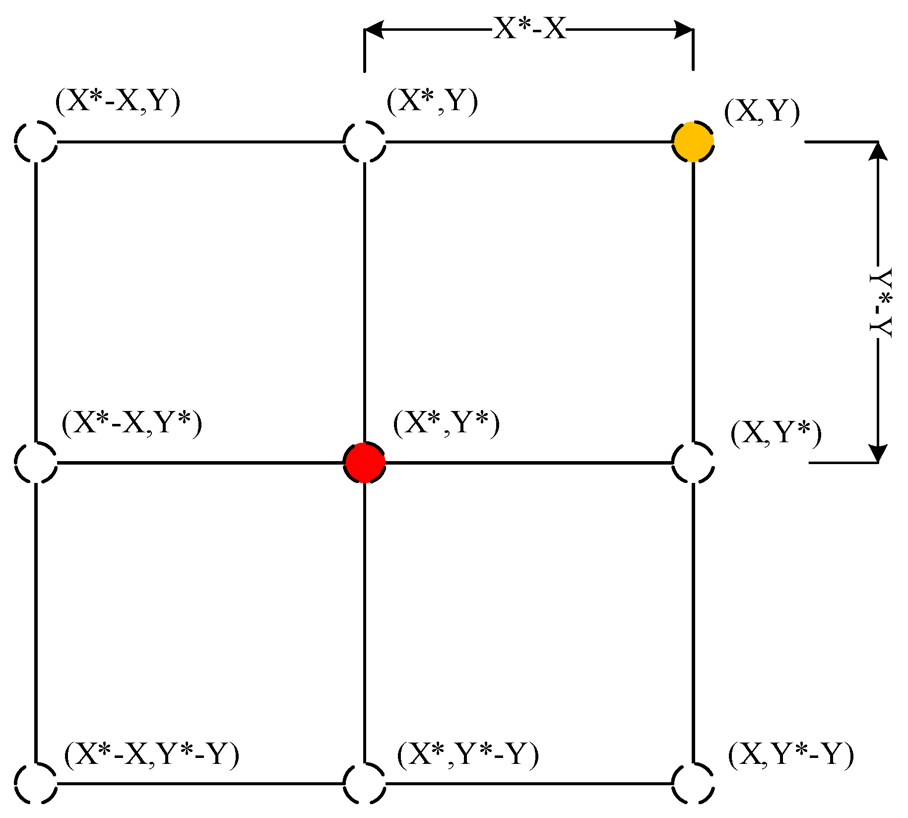
- Spiral updating position: This method first calculates the distance between the whale individual located at (X,Y) and the prey located at (X*,Y*). Then, a spiral equation is established between the two positions, thereby simulating the spiral movement pattern of the whale population. The equation is as follows:
- (3)
- Search Predation
3.2. LRWOA Algorithm
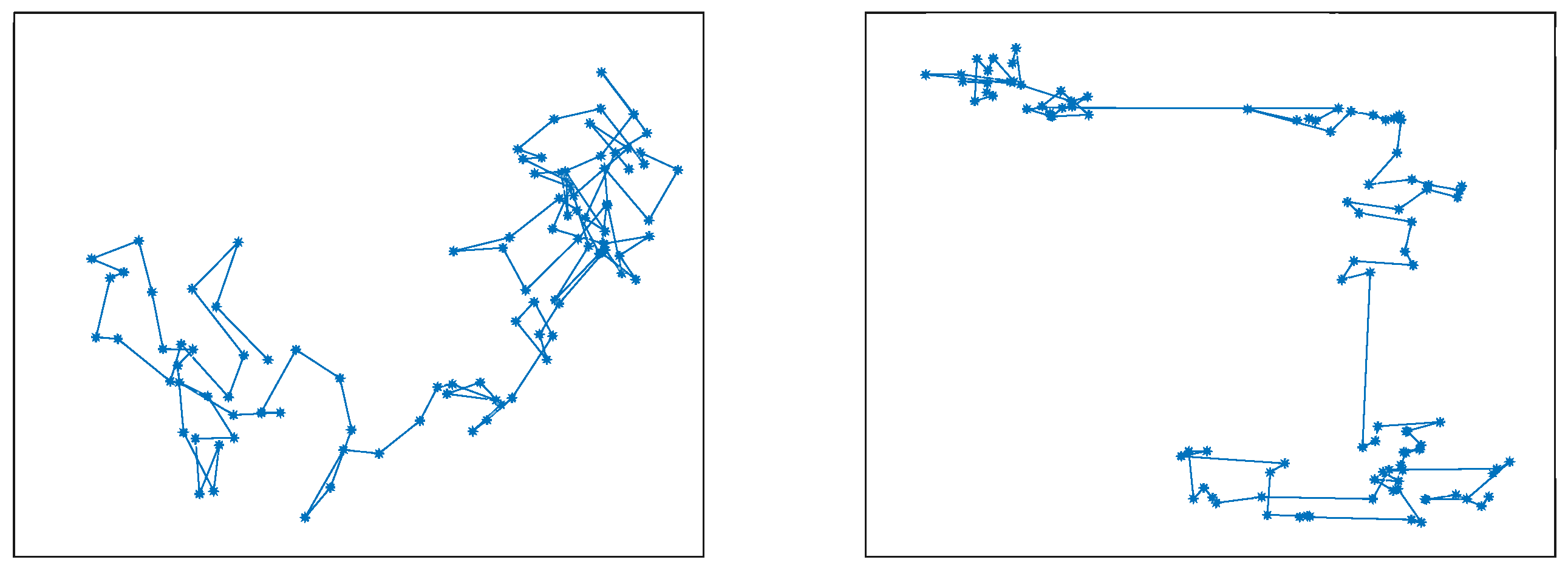
3.2.1. Lévy Flight Strategy
3.2.2. Random Walk Strategy
3.2.3. LRWOA
| Algorithm 1. LRWOA |
| Input: Number of whales , maximum number of iterations , iteration ratio Output: |
| Start: |
| 1: Initialize the whale population (k = 1, 2,...,N) in the search space. 2: Calculate the fitness values of the whale population individuals and select the best individual , the second best individual , and the third best individual . 3: Select a random individual rand and record its position. 4: while 5: for to perform 6: Calculate the values of parameters and according to and 7: if (X= =||X= =||X= =) perform 8: if (rand < ) perform 9: Adjust the positions by . 10: else 11: Adjust the positions by . 12: end if 13: Select the better positions based on . 14: end if 15: Update the individuals’ positions based on Equations (15) to (23). 16: end for 17: Calculate the fitness of individuals, update whale positions, and record the positions. 18: 19: end while |
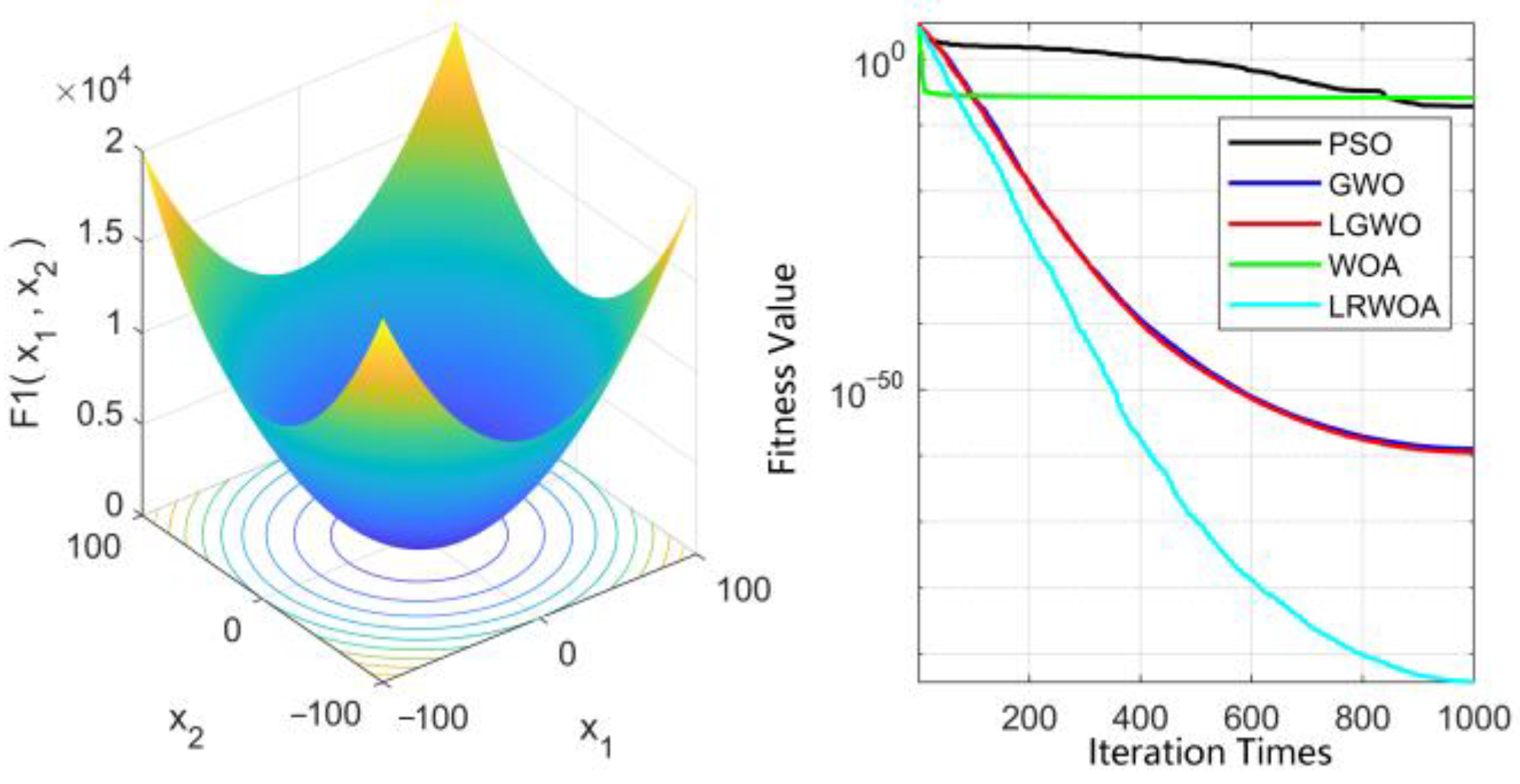
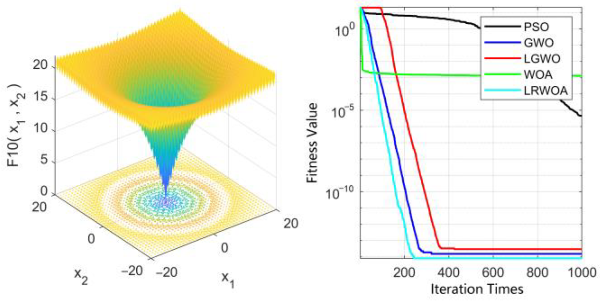
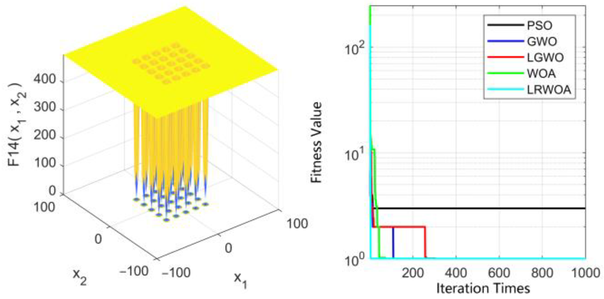
3.2.4. Results and Analysis
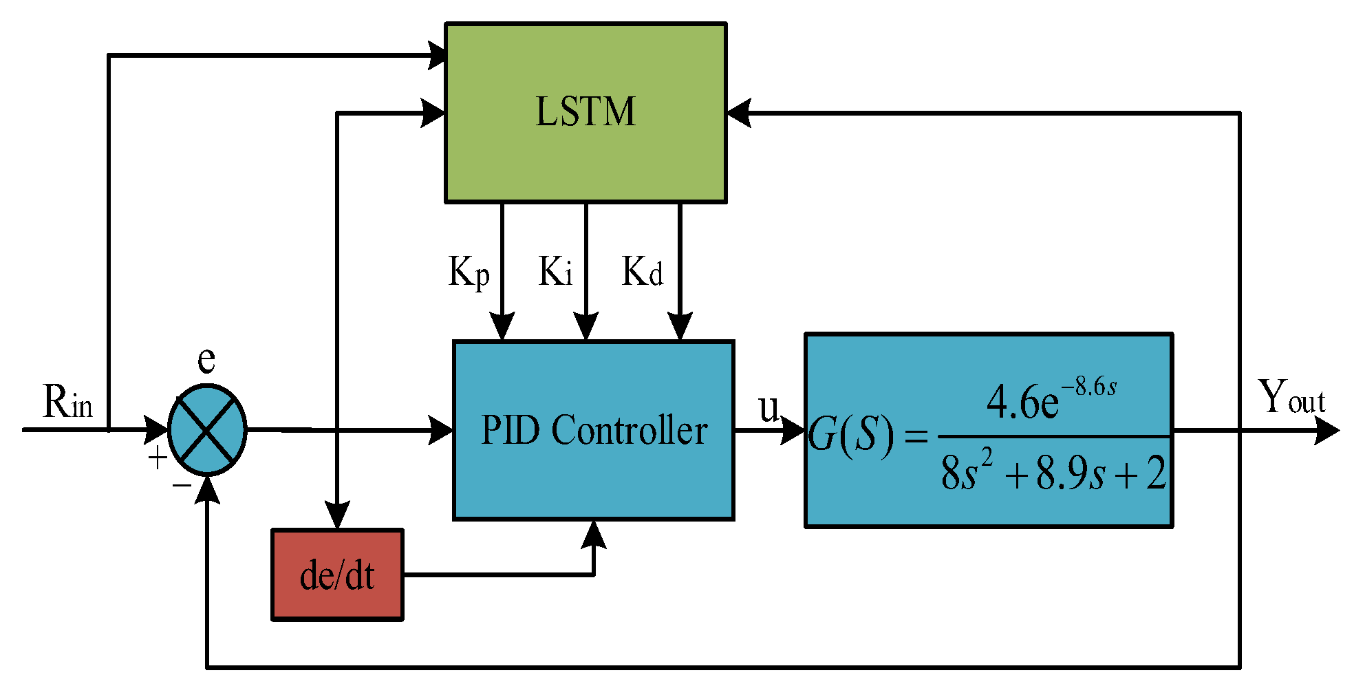
4. LRWOA-LSTM-PID Controller
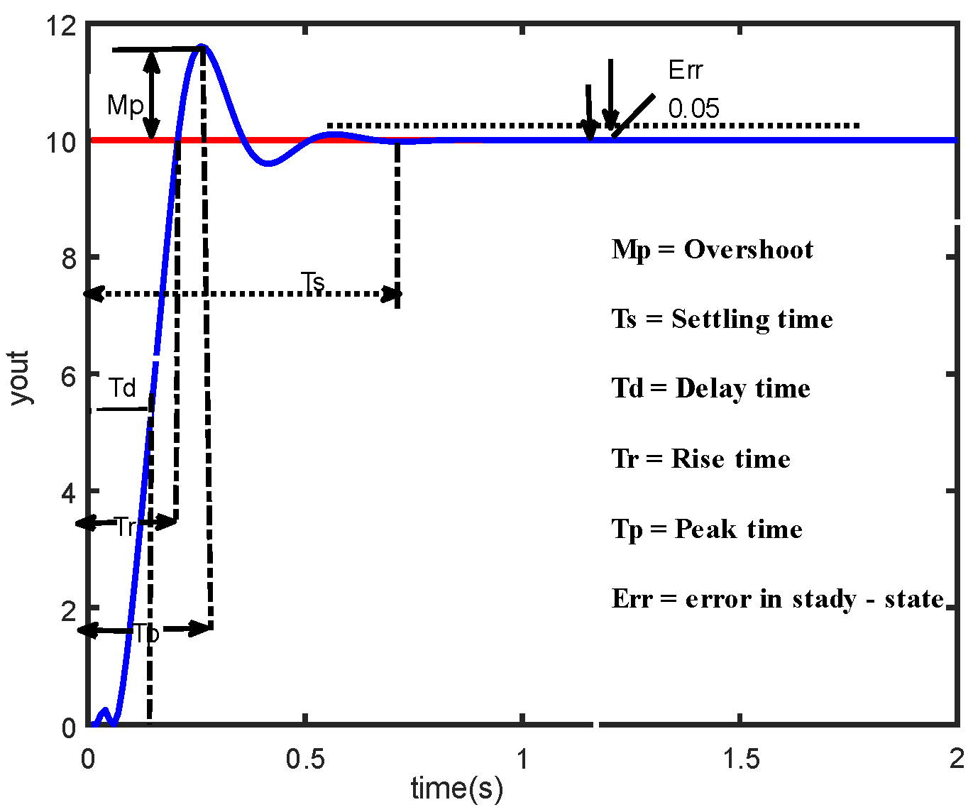
4.1. PID Controller
4.2. LSTM-PID Controller
4.2.1. The Forward Propagation of LSTM
4.2.2. The Backpropagation of the LSTM
4.2.3. PID Parameter Tuning Based on LSTM
4.3. LSTM-PID Controller Based on LRWOA Algorithm
5. Experiment
5.1. Parameter Description
5.2. Experimental Results and Analysis
6. Conclusions
Author Contributions
Funding
Data Availability Statement
Conflicts of Interest
References
- Ferraboschi, P.; Ciceri, S.; Grisenti, P. Applications of Lysozyme, an Innate Immune Defense Factor, as an Alternative Antibiotic. Antibiotics 2021, 10, 1534. [Google Scholar] [CrossRef] [PubMed]
- Mandal, A.; Herr, J.C. Preparation of Active Human Lysozyme and Transgenic Organisms. Patent No. WO2006028497, 16 March 2006. [Google Scholar]
- Ercan, D.; Demirci, A. Recent Advances for the Production and Recovery Methods of L-ysozyme. Crit. Rev. Biotechnol. 2016, 36, 1078–1088. [Google Scholar] [CrossRef] [PubMed]
- Zhu, X.; Zhu, Z. The Generalized Predictive Control of Bacteria Concentration in Marine Lysozyme Fermentation Process. Food Sci. Nutr. 2018, 6, 2459–2465. [Google Scholar] [CrossRef]
- Lasanta, C.; Roldán, A.; Caro, I.; Pérez, L.; Palacios, V. Use of Lysozyme for the Preve-ntion and Treatment of Heterolactic Fermentation in the Biological Aging of Sherry Wines. Food Control 2010, 21, 1442–1447. [Google Scholar] [CrossRef]
- Srikar, K.V.P.; Kumar, Y.V.P.; Pradeep, D.J.; Reddy, C.P. Investigation on PID Controller Tuning Methods for Aircraft Fuselage Temperature Control. In Proceedings of the 2020 International Symposium on Advanced Electrical and Communication Technologies (ISAECT), Kenitra, Morocco, 25–27 November 2020; pp. 1–5. [Google Scholar]
- Wu, X.; Wang, X.; He, G. A Fuzzy Self-Tuning Temperature PID Control Algorithms for 3D Bio-Printing Temperature Control System. In Proceedings of the 2020 Chinese Control And Decision Conference (CCDC), Hefei, China, 22–24 August 2020; pp. 2846–2849. [Google Scholar]
- Nasir, A.H.A.; Hambali, N.; Rahiman, M.H.F. Implementation of PRBS & RGS Perturbat-ion Input Signals on Steam Temperature: Model Estimation and PID Control. In Proceedings of the 2023 19th IEEE International Colloquium on Signal Processing & Its Applications (CSPA), Kedah, Malaysia, 3–4 March 2023; pp. 99–104. [Google Scholar]
- Wu, X.; Wu, J.; Li, D. Designation and Simulation of Environment Laboratory Temperature Control System Based on Adaptive Fuzzy PID. In Proceedings of the 2018 IEEE 3rd Advanced Information Technology, Electronic and Automation Control Conference (IAEAC), Chongqing, China, 12–14 October 2018; pp. 583–587. [Google Scholar]
- Åström, K.J.; Hägglund, T. Revisiting the Ziegler–Nichols Step Response Method for PID Control. J. Process Control 2004, 14, 635–650. [Google Scholar] [CrossRef]
- Franco, S.S.; Henríquez, J.R.; Ochoa, A.A.V.; da Costa, J.A.P.; Ferraz, K.A. Thermal Analysis and Development of PID Control for Electronic Expansion Device of Vapor Compression Refrigeration Systems. Appl. Therm. Eng. 2022, 206, 118130. [Google Scholar] [CrossRef]
- Muresan, C.I.; De Keyser, R. Revisiting Ziegler–Nichols. A Fractional Order Approach. ISA Trans. 2022, 129, 287–296. [Google Scholar] [CrossRef] [PubMed]
- Han, J.; Shan, X.; Liu, H.; Xiao, J.; Huang, T. Fuzzy Gain Scheduling PID Control of a Hybrid Robot Based on Dynamic Characteristics. Mech. Mach. Theory 2023, 184, 105283. [Google Scholar] [CrossRef]
- Bu, Q.; Cai, J.; Liu, Y.; Cao, M.; Dong, L.; Ruan, R.; Mao, H. The Effect of Fuzzy PID Temperature Control on The-rmal Behavior Analysis and Kinetics Study of Biomass Microwave Pyrolysis. J. Anal. Appl. Pyrolysis 2021, 158, 105176. [Google Scholar] [CrossRef]
- Singhal, K.; Kumar, V.; Rana, K.P.S. Robust Trajectory Tracking Control of Non-Holonomic Wheeled Mobile Robots Using an Adaptive Fractional Order Parallel Fuzzy PID Controller. J. Frankl. Inst. 2022, 359, 4160–4215. [Google Scholar] [CrossRef]
- Wei, Y.; Wu, Y.; Zhang, X.; Ren, J.; An, D. Fuzzy Self-Tuning PID-Based Intelligent Control of an Anti-Wave Buoy Data Acquisition Control System. IEEE Access 2019, 7, 166157–166164. [Google Scholar] [CrossRef]
- Jia, L.; Zhao, X. An Improved Particle Swarm Optimization (PSO) Optimized Integral Separation PID and Its Application on Central Position Control System. IEEE Sens. J. 2019, 19, 7064–7071. [Google Scholar] [CrossRef]
- Tang, G.; Lei, J.; Du, H.; Yao, B.; Zhu, W.; Hu, X. Proportional-Integral-Derivative Controller Optimization by Particle Swarm Optimization and Back Propagation Neural Network for a Parallel Stabilized Platform in Marine Operations. J. Ocean Eng. Sci. 2022. [Google Scholar] [CrossRef]
- Feng, H.; Ma, W.; Yin, C.; Cao, D. Trajectory Control of Electro-Hydraulic Position Servo System Using Improved PSO-PID Controller. Autom. Constr. 2021, 127, 103722. [Google Scholar] [CrossRef]
- Mohamed, M.A.; Eltamaly, A.M.; Alolah, A.I. PSO-Based Smart Grid Application for Sizing and Optimization of Hybrid Renewable Energy Systems. PLoS ONE 2016, 11, e0159702. [Google Scholar] [CrossRef]
- Lin, C.L.; Jan, H.Y.; Shieh, N.C. GA-Based Multiobjective PID Control for a Linear Brushless DC Motor. IEEE/ASME Trans. Mechatron. 2003, 8, 56–65. [Google Scholar] [CrossRef]
- Hussain, M.; Aparna, V.; Shajahan, M.S.M.; Jamal, D.N. Tuning of PID Controller Using GA, SA and QFT for Three Interacting Tank Process. In Proceedings of the 2018 2nd International Conference on Trends in Electronics and Informatics (ICOEI), Tirunelveli, India, 11–12 May 2018; pp. 549–553. [Google Scholar]
- Elbayomy, K.M.; Zongxia, J.; Huaqing, Z. PID Controller Optimization by GA and Its Performances on the Electro-Hydraulic Servo Control System. Chin. J. Aeronaut. 2008, 21, 378–384. [Google Scholar] [CrossRef]
- Mousakazemi, S.M.H. Comparison of the Error-Integral Performance Indexes in a GA-Tuned PID Controlling System of a PWR-Type Nuclear Reactor Point-Kinetics Model. Prog. Nucl. Energy 2021, 132, 103604. [Google Scholar] [CrossRef]
- Sinha, N.; Lai, L.L.; Rao, V.G. Venu Gopal Rao GA Optimized PID Controllers for Automatic Generation Control of Two Area Reheat Thermal Systems under Deregulated Environment. In Proceedings of the 2008 Third International Conference on Electric Utility Deregulation and Restructuring and Power Technologies, Nanjing, China, 6–9 April 2008; pp. 1186–1191. [Google Scholar]
- Li, G.; Guo, C.; Li, Y.; Deng, W. Fractional-Order PID Controller of USV Course-Keeping Using Hybrid GA-PSO Algorithm. In Proceedings of the 2015 8th International Symposium on Computational Intelligence and Design (ISCID), Hangzhou, China, 12–13 December 2015; Volume 2, pp. 506–509. [Google Scholar]
- Cheng, C.-H.; Cheng, P.-J.; Xie, M.-J. Current Sharing of Paralleled DC–DC Converters Using GA-Based PID Controllers. Expert Syst. Appl. 2010, 37, 733–740. [Google Scholar] [CrossRef]
- Mohamad Ali Tousi, S.; Mostafanasab, A.; Teshnehlab, M. Design of Self Tuning PID Controller Based on Competitional PSO. In Proceedings of the 2020 4th Conference on Swarm Intelligence and Evolutionary Computation (CSIEC), Mashhad, Iran, 2–4 September 2020; pp. 022–026. [Google Scholar]
- Xue, H.; Bai, Y.; Hu, H.; Xu, T.; Liang, H. A Novel Hybrid Model Based on TVIW-PSO-GSA Algorithm and Support Vector Machine for Classification Problems. IEEE Access 2019, 7, 27789–27801. [Google Scholar] [CrossRef]
- Agatonovic-Kustrin, S.; Beresford, R. Basic Concepts of Artificial Neural Network (ANN) Modeling and Its Application in Pharmaceutical Research. J. Pharm. Biomed. Anal. 2000, 22, 717–727. [Google Scholar] [CrossRef] [PubMed]
- Varghese, M.M.; Vakamalla, T.R.; Gujjula, R.; Mangadoddy, N. Prediction of Solid Circulation Rate in an Internal Circulating Fluidized Bed: An Empirical and ANN Approach. Flow Meas. Instrum. 2022, 88, 102274. [Google Scholar] [CrossRef]
- Liu, Z.; Liang, J.; Zhang, S.; Kayacan, E. ANN-Based Vibration Control of an Aerial Refueling Hose System with Input Nonlinearity and Prescribed Output Constraint. J. Frankl. Inst. 2022, 359, 2627–2645. [Google Scholar] [CrossRef]
- Wu, W.; Dandy, G.C.; Maier, H.R. Protocol for Developing ANN Models and Its Application to the Assessment of the Quality of the ANN Model Development Process in Drinking Water Quality Modelling. Environ. Model. Softw. 2014, 54, 108–127. [Google Scholar] [CrossRef]
- Huang, G.; Yuan, X.; Shi, K.; Wu, X. A BP-PID Controller-Based Multi-Model Control System for Lateral Stability of Distributed Drive Electric Vehicle. J. Frankl. Inst. 2019, 356, 7290–7311. [Google Scholar] [CrossRef]
- Anh, H.P.H.; Nam, N.T.; Anh, H.P.H.; Nam, N.T. A New Approach of the Online Tuning Gain Scheduling Nonlinear PID Controller Using Neural Network. In PID Control, Implementation and Tuning; IntechOpen: Rijeka, Croatia, 2011; ISBN 978-953-307-166-4. [Google Scholar]
- Asgharnia, A.; Jamali, A.; Shahnazi, R.; Maheri, A. Load Mitigation of a Class of 5-MW Wind Turbine with RBF Neural Network Based Fractional-Order PID Controller. ISA Trans. 2020, 96, 272–286. [Google Scholar] [CrossRef] [PubMed]
- Dhaouadi, R.; Jafari, R. Adaptive PID Neuro-Controller for a Nonlinear Servomechanism. In Proceedings of the 2007 IEEE International Symposium on Industrial Electronics, Vigo, Spain, 4–7 June 2007; pp. 157–162. [Google Scholar]
- Zhang, G.; Lu, R.; Chen, M. A Stable Self-Learning DRNN-PID Control of Multi-Point Mooring System. In Proceedings of the Advances in Guidance, Navigation and Control, Harbin, China, 5–7 August 2022; Yan, L., Duan, H., Yu, X., Eds.; Springer: Singapore, 2022; pp. 4769–4779. [Google Scholar]
- Meng, Z.; Zhang, L.; Wang, H.; Ma, X.; Li, H.; Zhu, F. Research and Design of Precision Fertilizer Application Control System Based on PSO-BP-PID Algorithm. Agriculture 2022, 12, 1395. [Google Scholar] [CrossRef]
- Jin, L.; Fan, J.; Du, F.; Zhan, M. Research on Two-Stage Semi-Active ISD Suspension Based on Improved Fuzzy Neural Network PID Control. Sensors 2023, 23, 8388. [Google Scholar] [CrossRef] [PubMed]
- Mirjalili, S.; Lewis, A. The Whale Optimization Algorithm. Adv. Eng. Softw. 2016, 95, 51–67. [Google Scholar] [CrossRef]
- Dubkov, A.A.; Spagnolo, B.; Uchaikin, V.V. Lévy Flight Superdiffusion: An Introduction. Int. J. Bifurc. Chaos 2008, 18, 2649–2672. [Google Scholar] [CrossRef]
- Geim, A.K. Nobel Lecture: Random Walk to Graphene. Rev. Mod. Phys. 2011, 83, 851–862. [Google Scholar] [CrossRef]
- Shi, Y.; Eberhart, R.C. Parameter Selection in Particle Swarm Optimization. In Proceedings of the Evolutionary Programming VII, San Diego, CA, USA, 25–27 March 1998; Porto, V.W., Saravanan, N., Waagen, D., Eiben, A.E., Eds.; Springer: Berlin/Heidelberg, Germany, 1998; pp. 591–600. [Google Scholar]
- Zhang, M.; Zhang, W.; Wang, J.; Xiong, X.; Cheng, Y.; Lv, X. Reconstructions of Strain Distribution along FBG Sensor Using GWO Algorithm and Interrelated Simulation Verification. In Proceedings of the 2022 IEEE International Conference on Sensing, Diagnostics, Prognostics, and Control (SDPC), Chongqing, China, 5–7 August 2022; pp. 1–5. [Google Scholar]
- Luo, J.; Chen, H.; Wang, K.; Tong, C.; Li, J.; Cai, Z. LGWO: An Improved Grey Wolf Optimization for Function Optimization. In Proceedings of the Advances in Swarm Intelligence, Fukuoka, Japan, 27 July 27–1 August 2017; Tan, Y., Takagi, H., Shi, Y., Eds.; Springer International Publishing: Cham, Switzerland, 2017; pp. 99–105. [Google Scholar]


| Function Type | Index | Function Name | Search Range | Adaptive Value |
|---|---|---|---|---|
| single-peak functions | F1 | Sphere Function | [−100, 100] | 0 |
| F2 | Schwefel’s Problem 1.2 | [−100, 100] | 0 | |
| F3 | Schwefel’s Problem 1.2 With Noise | [−32, 32] | 0 | |
| F4 | Schwefel’s Problem 2.21 | [−5, 5] | 0 | |
| F5 | Schwefel’s Problem 2.22 | [−10, 10] | 0 | |
| F6 | High Conditioned Elliptic Function | [−3, 1] | 0 | |
| F7 | Step Function | [−10, 10] | 0 | |
| multi-peak functions | F8 | Schwefel Function | [−500, 500] | 0 |
| F9 | Rosenbrock’s Function | [−10, 10] | 0 | |
| F10 | Quartic Function | [2, 5] | 0 | |
| F11 | Griewank’s Function | [−600, 600] | 0 | |
| F12 | Ackley’s Function | [−32, 32] | 0 | |
| F13 | Rastrign’s Function | [−5.12, 5.12] | 0 | |
| F14 | Rastrign’s Noncontinue Function | [−5.12, 5.12] | 0 | |
| F15 | Weierstrass Function | [−100, 100] | 0 |
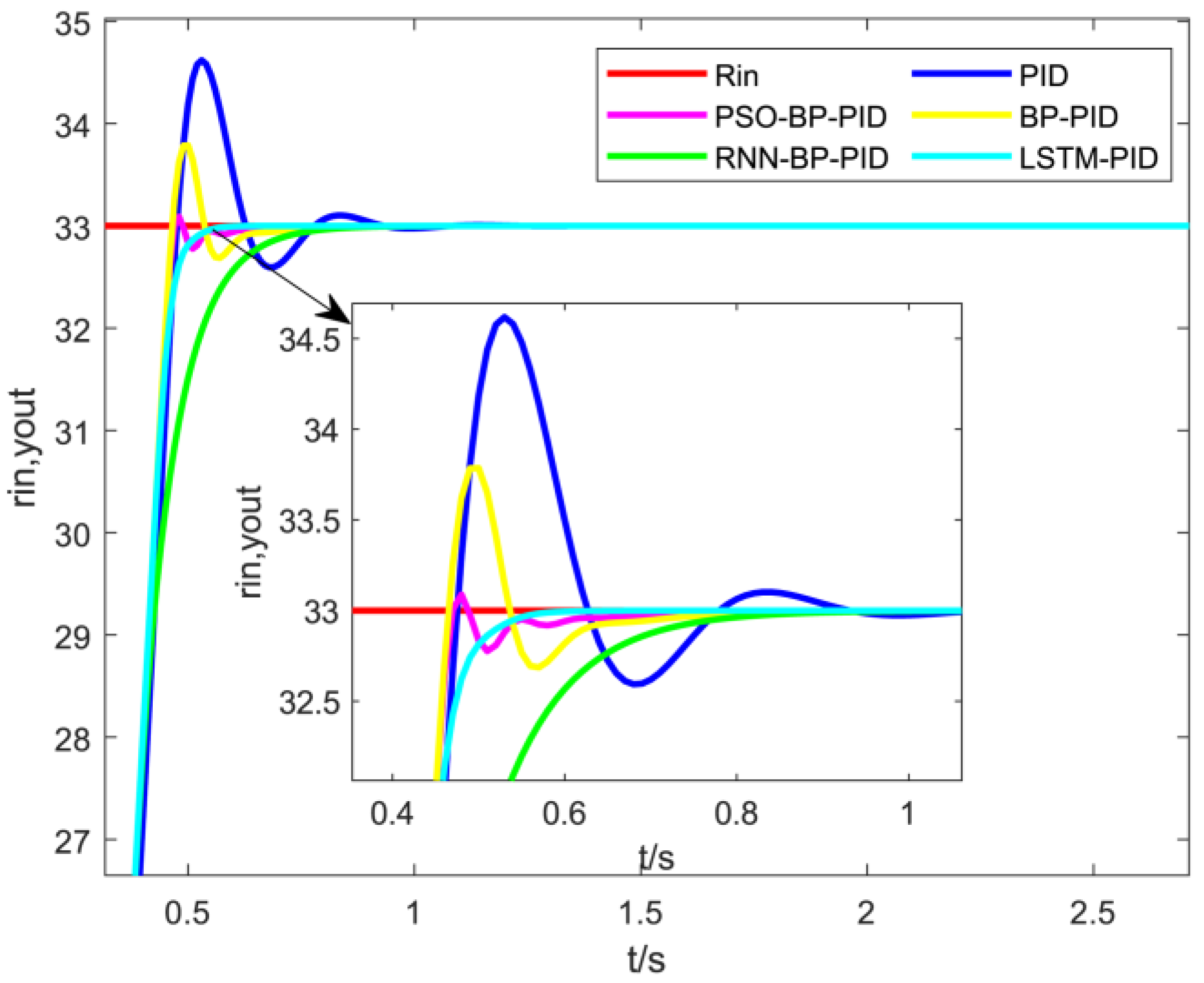
| CONTROLLER | PID | BP-PID | PSO-BP-PID | RNN-BP-PID | LSTM-PID |
|---|---|---|---|---|---|
| Rise time (s) | 0.48 | 0.46 | 0.47 | 0.77 | 0.61 |
| Settling time (s) | 1.06 | 0.74 | 0.72 | 0.77 | 0.61 |
| Overshoot (°C) | 1.62 | 0.79 | 0.10 | 0.00 | 0.00 |
| Peak (°C) | 34.62 | 33.79 | 33.10 | 33.00 | 33.00 |
| Peak time (s) | 0.53 | 0.50 | 0.48 | 0.77 | 0.61 |
| Kp | 4.08 | 9.91 | 2.51 | 14.82 | 10.01 |
| Ki | 0.87 | 1.92 | 1.72 | 1.8 | 2.09 |
| Kd | 12.00 | 9.46 | 10.03 | 10.4 | 10.06 |
| Error | 0 | 0 | 0 | 0 | 0 |
| CONTROLLER | LSTM-PID | LRWOA-LSTM-PID |
|---|---|---|
| Rise time (s) | 0.61 | 0.55 |
| Settling time (s) | 0.61 | 0.55 |
| Overshoot (%) | 0.00 | 0.00 |
| Peak (°C) | 33.00 | 33.00 |
| Peak time (s) | 0.61 | 0.55 |
| Kp | 10.01 | 12.02 |
| Ki | 2.09 | 3.04 |
| Kd | 10.06 | 11.20 |
| Error | 0 | 0 |
Disclaimer/Publisher’s Note: The statements, opinions and data contained in all publications are solely those of the individual author(s) and contributor(s) and not of MDPI and/or the editor(s). MDPI and/or the editor(s) disclaim responsibility for any injury to people or property resulting from any ideas, methods, instructions or products referred to in the content. |
© 2024 by the authors. Licensee MDPI, Basel, Switzerland. This article is an open access article distributed under the terms and conditions of the Creative Commons Attribution (CC BY) license (https://creativecommons.org/licenses/by/4.0/).
Share and Cite
Ding, C.; Li, X.; Zhou, H.; Yu, J.; Du, J.; Zhao, S. A Temperature Control Method of Lysozyme Fermentation Based on LRWOA-LSTM-PID. Processes 2024, 12, 866. https://doi.org/10.3390/pr12050866
Ding C, Li X, Zhou H, Yu J, Du J, Zhao S. A Temperature Control Method of Lysozyme Fermentation Based on LRWOA-LSTM-PID. Processes. 2024; 12(5):866. https://doi.org/10.3390/pr12050866
Chicago/Turabian StyleDing, Chenhua, Xungen Li, Hanlin Zhou, Jianming Yu, Juling Du, and Shixiang Zhao. 2024. "A Temperature Control Method of Lysozyme Fermentation Based on LRWOA-LSTM-PID" Processes 12, no. 5: 866. https://doi.org/10.3390/pr12050866
APA StyleDing, C., Li, X., Zhou, H., Yu, J., Du, J., & Zhao, S. (2024). A Temperature Control Method of Lysozyme Fermentation Based on LRWOA-LSTM-PID. Processes, 12(5), 866. https://doi.org/10.3390/pr12050866