Complex Environment Based on Improved A* Algorithm Research on Path Planning of Inspection Robots

Abstract

The proposed research aims to accomplish an improved A* algorithm for mobile robots in complex environments. In this novel algorithm, the guidance of environment information is added to the evaluation function to enhance the adaptability of the algorithm in complex environments. Additionally, to solve the problem of path smoothness, the optimal selection rules for child nodes and the bidirectional optimization strategy for path smoothing are introduced to reduce redundant nodes, which effectively makes the search space smaller and the path smoother. The simulation experiments show that, compared with the colony algorithm and Dijkstra algorithms, the proposed algorithm has significantly improved performance. Compared with the A* algorithm, the average planning time is reduced by 17.2%, the average path length is reduced by 2.05%, the average turning point is reduced by 49.4%, and the average turning Angle is reduced by 75.5%. The improved A* algorithm reduces the search space by 61.5% on average. The simulation results show that the effectiveness and adaptability of the improved A* algorithm in complex environments are verified by multi-scale mapping and multi-obstacle environment simulation experiments.

1. Introduction

The performance of the algorithm directly determines the robot’s autonomous navigation ability and task completion efficiency in complex environments [1]. According to the master’s degree and analysis ability of environment information, two kinds of path planning algorithms can be distinguished. One is the global path planning algorithm with fully known environmental information, such as the A* algorithm, ant colony algorithm, genetic algorithm [2,3,4], etc. The other type is local path planning algorithms that are partially or completely unknown to environmental information, such as the D* algorithm, artificial potential field algorithm, DWA algorithm [5,6,7], etc.

Aiming at problems such as low search efficiency, redundancy of search nodes, and the uneven path of the A* algorithm in path planning under large-scale maps, Song et al. [8] studied path planning of autonomous ships under an open environment and improved path node optimization using the A* algorithm to make the entire route smoother and lower overall energy consumption. Phan Gia Luan et al. adopted a multi-level A* algorithm to add a dynamic obstacle weighting model for obstacle avoidance at the second layer and Bezier curves for path smoothing at the first layer [9]. To achieve obstacle avoidance and path smoothing, Zuo et al. [10] implemented layered A* in 2015. The first layer uses the A* algorithm for initial path planning, and the second layer uses an approximate method for local path correction. The combination of A* algorithms has been demonstrated in numerous studies, and the grid method is widely used [11]. The main objective of the research is to reduce the number of path nodes and improve the smoothness of the path. There is a feature to sort maps. Combining the A* algorithm with the Voronoi diagram, the path quality is improved significantly. However, due to the inability of map modeling methods to identify the shape of obstacles, obstacle avoidance technology faces great challenges. Oluwaseun Opeyemi Martins et al. [12] added the multi-object recognition method to design an AMO Astar algorithm that can be used in large-scale workspace scenes. Jose Lima et al. [13] selected five common daily work scenarios as the template graph, specified the corresponding weight coefficient, customized the sum of time cost and distance cost, and reduced the search time. Ji Xu [14] et al. added the weight information of the road surface, proposed the idea of extracting transition nodes, and deleted some redundant nodes. It can effectively avoid unnecessary road bumps, eliminate redundant inflection points, improve path smoothness, increase path smoothness, and achieve a compromise between path length and road relief.

To make the robot detect comprehensively and efficiently, a suitable global path planning algorithm is needed to shorten the overall motion time of the robot. LIU et al. [15,16] proposed a method of mine flood escape path planning based on the improved bidirectional A* algorithm, which can obtain an escape path with fewer redundant nodes and a smaller turning angle, but the path lacks smoothness. QI et al. [17,18] introduced the weight coefficient of the heuristic function to set the safe distance of obstacles and improved the obstacle avoidance performance of the algorithm. Based on the idea of calculating the slope between sampling points, a path smoothing algorithm is designed, which removes redundant nodes and reduces the path transition but does not reduce the algorithm time. Aiming at the path planning problem of mobile robots in the complex environment of multi-scale maps and multi-type obstacles, Y Zhou [19] applied a Q-learning algorithm to the path planning of mobile robots in 2022. Aiming at the blindness of the mobile robot exploration environment, the RRT algorithm is combined and improved to improve the goal-oriented performance of the robot exploration environment. To overcome the problem of slow convergence of classical Q-learning, parameters such as exploration rate, discount rate, and learning rate are modified. An improved ant colony optimization algorithm is designed to enable robots to consider the information of other robots and improve the accuracy of action decisions. The hierarchical thought of the gray wolf optimization algorithm is introduced into the improved ant colony algorithm to realize the dynamic regulation of pheromones. Aiming at the problem that path planning is likely to fail and be ineffective in special terrain under complex environments and there being no safe distance, Bian Yongming et al. [20] modified the evaluation subfunction to improve the passing ability of the improved algorithm under the “U” trap. Wang Bin et al. [4] introduced the parent node information and integrated the A* algorithm, which not only increased the heuristic of the algorithm but also improved the local planning ability. Zhan Jingwu [5] et al. introduced the safe distance factor into the heuristic function of the A* algorithm and combined it with the dynamic window algorithm to improve the security of the planned path. Zhang Jianhua et al. [6] designed an algorithm that dynamically adjusts parameters according to speed and predicted distance to make the algorithm more flexible in path planning. Zhang Xiaoyi [21] proposed a combination algorithm inspired by the A* algorithm, which reduces the circuits that may appear in the port environment of AGV and improves operation efficiency. Zhang Yu [22] et al. constrained the velocity evaluation subfunction in the dynamic window algorithm to limit the acceleration threshold. At the same time, the error of the predicted path is compensated with the attitude information of the odometer, the deviation between the planned path and the optimal path is reduced, and the effectiveness of the algorithm in the parking lot environment is verified.

Omar et al. proposed in 2021 that when using the mixed group optimization algorithm to solve the path planning problem of mobile robots, the two main problems are obstacle collision on the path and path length reduction [23]. Ke Dagher et al. proposed the adaptive artificial neural network (ANN) control method in 2022 based on the online adjustment and evolutionary slice genetic algorithm, which is adopted to control the motion of a nonlinear dynamic mobile robot system [24]. In October 2022, Yang Zhang [25] proposed a new navigation system based on mobile robots, which combines vision and multi-line lidar information to ensure not only the richness of information but also the security and accuracy of map edge information. At the same time, it can also meet the real-time accurate positioning and navigation of logistics warehousing scenarios in complex environments. In 2021, Gao et al. [26] proposed to use the adaptive step size method and cubic Bezier curve to solve the multi-turning point problem. Xie et al. [27] proposed the dynamic selection iterative frequency method to solve the adaptability problem of robot path planning. In 2023, Hao et al. [28] proposed to use two-level method to solve the safety problem of UAV paths from both dynamic and static levels. Li et al. [29] proposed that HAGA and AGA algorithms deal with the problem of robot path planning for multi-task processing in complex environments. In 2024, Ye et al. [30] proposed that an improved LQR algorithm be used to optimize the A* algorithm to solve the problem of inaccurate paths in the field of robot automatic driving.

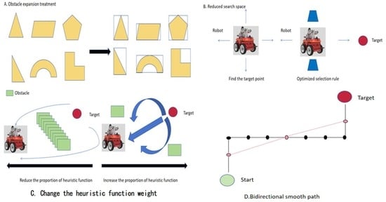
The traditional path planning algorithm has some disadvantages in application, such as a high computation time cost and a large computation amount of the traditional genetic algorithm. Due to the limitation of initial pheromone concentration, the traditional ant colony algorithm has a low initial search speed in path planning and can easily fall into the local optimal state. In the path planning of large-scale scenarios, there will be a large number of redundant nodes, which makes the loss of mobile robots too high. Therefore, this paper proposes an improved A* algorithm based on the traditional A* algorithm. Firstly, the improved heuristic function is used to remove the redundant nodes in the path search process, and the environment information parameters in the new heuristic function are used to enhance the adaptability of the robot to detect different paths. Then, the child node selection rules of the robot are optimized to ensure the obstacle avoidance of the planned path. Finally, the bidirectional smoothing optimization method between path nodes is used to adjust and optimize the planned path, delete the intermediate redundant nodes, reduce the transition, and improve the smoothness of the path. The smooth and continuous optimal path is generated to avoid unnecessary turns and pauses on the path so that the robot can complete the inspection task with higher speed and less energy consumption, greatly improving the inspection efficiency of the inspection robot in the complex environment.

2. Path Planning Algorithm

2.1. Map Environment Description

The premise of path planning is the drawing of an environment diagram. The grid method is widely used in the construction of robot workspace diagrams because of its simple operation and easy implementation. The grid method abstracts the actual working environment of the robot into a two-dimensional map, simplifying the operating space [31,32]. The importance of obstacle mesh size selection for the whole path planning should not be underestimated. The larger the mesh size selection, the larger the area represented by each mesh, the fewer the number of grids to be considered in path planning, and the less computation required. However, robots need to move through a larger grid, which can lead to unnecessary path extension, increasing path length. Conversely, if the grid is too small, information about the environment can be described more precisely, which helps avoid narrow passages that the robot cannot get through and smaller obstacles that it cannot get around. Although the accuracy of path planning is improved, more grids need to be considered and more complex searches and evaluations need to be carried out, which increases the amount of computation and slows down the planning process [33,34]. Therefore, this study divides the cell grid based on the map resolution. When path planning is carried out in a raster diagram, the robot is reduced to a point-like object moving on a two-dimensional plane. The rescue robot used in the research is rectangular, the center of gravity of the robot base is a particle, and the outside is a circle, as shown in Figure 1.

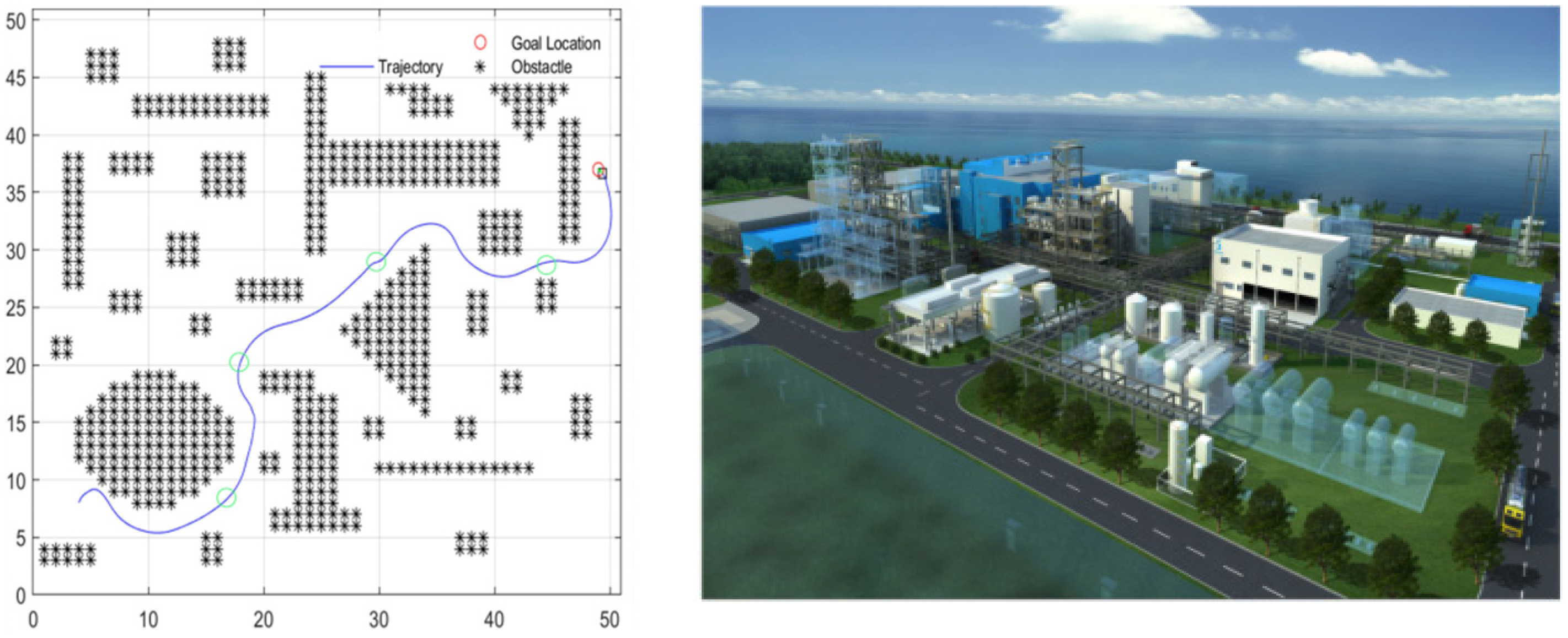
In Figure 2, the right picture is the internal environment diagram of a real chemical company, the left picture is the obstacle map corresponding to the optimization of the inspection robot, the lower left is the starting point, and the upper right is the endpoint. The green circle in the trajectory is the local node in the path.

There are rich types of scene information in complex environments, which are mainly divided into two directions: road information and obstacle information.

The road information includes the roughness of the road surface, the regularity of the route boundary, the slope of the traveling route, and the scale and traversability of the map composed of feasible areas. Obstacle information includes shape, size, number, distribution, static and dynamic state, and whether there are vital signs.

In order to improve the universality of the mobile robot path planning algorithm, the horizontal ground is chosen as the path planning information. This research identifies the complex environment as a collection of barriers with various types of obstacles that make up the obstacle information in the mobile robots’ path planning scene and multiple numbers and an uneven spatial and temporal distribution, that is, the number of obstacles in the scene is large and the shape is irregular.

To improve the universality of the mobile robot path planning algorithm, the horizontal ground is chosen as the path planning information. The road on the ground is composed of four attributes: one that the ordinary wheeled robot can normally pass, one that has no regular boundary constraints, one that is on flat ground, and one that is on a large scale. A set of obstacles with multiple types, multiple numbers, and an uneven spatial and temporal distribution is selected as the obstacle information, and the scene composed of the two is taken as the complex environment for research, and the map is constructed.

When constructing the raster map, the obstacle is processed according to its state under the raster map so that it is formatted and displayed in the raster map, which is easy to plan the path. The higher the accuracy of the raster map, the closer to the original obstacle information. As shown in Figure 3, when any part of the obstacle occupies the grid, the grid is set as the obstacle grid, and the mobile robot is not feasible in this area.2

The processed raster map is shown in Figure 4. The figure’s lower left corner represents the coordinate system’s origin. The x and y axes are representative of the horizontal and vertical directions, respectively. Figure 4’s white grid represents the open area that the robot can navigate, while the black grid represents a barrier that it cannot. Let the current position of the robot be M (i, j), and then the mathematical expression of the unit grid is as follows:

$$M(i,j)=\left\{\begin{array}{cc}0\hfill & (\mathrm{Free} \mathrm{lattice})\\ 1\hfill & \left(\mathrm{obstacle}\right)\end{array}\right.$$

(1)

2.2. Path Planning of the Traditional A* Algorithm

The A* algorithm is a heuristic search algorithm, which has the characteristics of high search efficiency, fast planning speed, and overcoming the precocious phenomenon formed in the search process, and it is widely used in the solution of the optimal path. The search principle of the A* algorithm is mainly to search the sub-grid points around the starting grid point from the starting grid point each time from the surrounding sub-grid points to select a point with the lowest evaluation function as the next search node, that is, the current node. The sub-grid points adjacent to the current node are generated again, and the lowest point of the evaluation function is re-searched for the new current node, and the search is sequential until the current node is the destination location.

The A* algorithm defines two list storage raster nodes related to the search path, namely, the OPEN storage table and the CLOSED storage table. The OPEN table holds the search space of all reachable access nodes, that is, path nodes. The CLOSED table stores the smallest child node of each evaluation function. The evaluation function influences the frequency of generation of the current node, and the OPEN table is accessed every time the current node is updated. The evaluation function affects the size of the search space, and the size of the search space and the number of visits affect the speed of the A* algorithm. Hence, the path planning outcome and search efficiency are directly impacted by the A* algorithm’s evaluation function. Let $f(n)$ be the evaluation function of the A* algorithm; the formula is as follows:

$$f(n)=g(n)+h(n)$$

(2)

where $g(n)$ is the cost function of the sum between the starting position and the current position $n$, $h(n)$ is the heuristic function that estimates the path cost between the current section location $n$, and the destination location.

The evaluation function $f(n)$ uses accuracy as a key part of the effectiveness and performance of the A* algorithm’s path planning. As can be seen in Formula (2), the evaluation function $f(n)$ is jointly determined by the cost function $g(n)$ and the heuristic function $h(n)$, and its characteristics are as follows:

(1)

If the heuristic function is $h(n)=0$, only $g(n)$ works, and the search index only calculates the path distance cost from the starting position to the current position and does not calculate the cost to the destination position, which belongs to a single computational search. At this point, the A* algorithm evolved into Dijkstra’s algorithm.

(2)

If the value estimated by the heuristic function $h(n)$ is smaller than the actual cost, the algorithm can ensure that a path with the least cost is found, but its search space and search time will increase accordingly. That is, with the $h(n)$ decrease in the A* algorithm, there will be more and more optional nodes in the storage space, resulting in a decrease in the algorithm’s operation speed.

(3)

If the value estimated by the heuristic function $h(n)$ is the same as the value of the actual cost, the algorithm only searches the nodes on the optimal path without generating redundant search nodes, so the algorithm is fast at this time.

(4)

When the estimated value of the heuristic function $h(n)$ is larger than the actual cost, the algorithm can find the path with the shortest distance. However, the algorithm can be very fast. If $h(n)$ is much larger than $g(n)$, only $h(n)$ works, and the A* algorithm evolves into a breadth-first search (BFS).

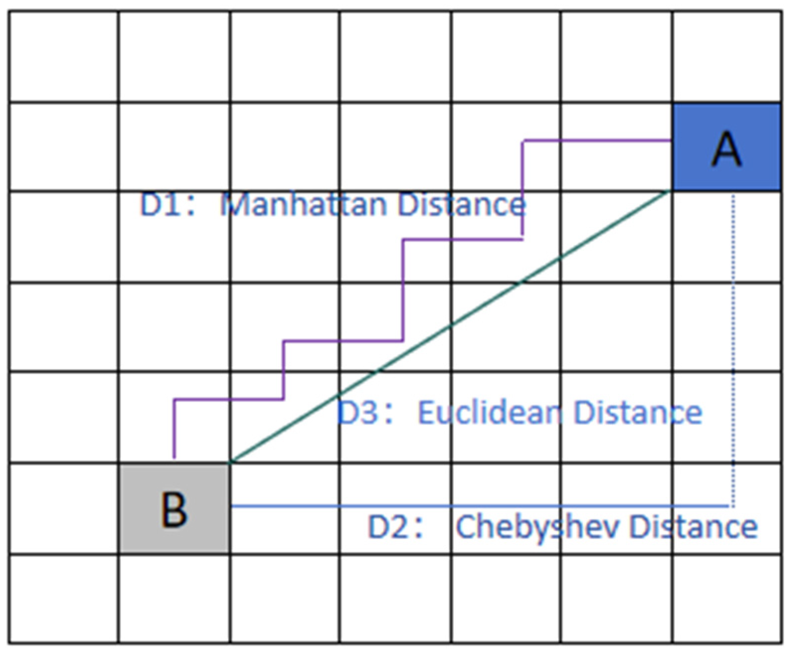
Therefore, the search of the A* algorithm is flexible, and the speed and accuracy of the algorithm can be controlled by adjusting the heuristic function. The A* algorithm optimizes its heuristic function $h(n)$ according to different requirements of path planning to increase the algorithm’s efficiency. Common heuristic function expressions are Manhattan distance, Chebyshev distance, and Euclidean distance, as shown in Figure 5.

Suppose that the coordinates of any two points A $(x_i,y_i)$ and B $(x_j,y_j)$ in the plane cartesian coordinate system are, respectively, sum, and let the distance be denoted as $D$.

(1)

Manhattan Distance

Manhattan Distance: The total of the absolute value of the difference between the coordinates of two points, A and B, in the horizontal and vertical directions, as shown in Figure 5 for route D1. The expression is as follows:

$$D_{AB}=\left|x_i-x_j\right|+\left|y_i-y_j\right|$$

(3)

(2)

Chebyshev Distance:

Chebyshev Distance: The absolute value of the maximum difference between the horizontal and vertical coordinates of coordinates of two points, A and B, as shown in Figure 5 for route D2. The expression is as follows:

$$D_{AB}=\max \left\{\left|x_i-x_j\right|,\left|y_i-y_j\right|\right\}$$

(4)

(3)

Euclidean Distance:

Euclidean Distance: The linear distance between the coordinates of two points, A and B, as shown in Figure 5 for route D3. The expression is as follows:

$$D_{AB}=\sqrt{{(x_i-x_j)}^2+{(y_i-y_j)}^2}$$

(5)

According to the relationship between the heuristic function and the A* algorithm’s performance, the predicted path using the Euclidean distance equals the real shortest path if there are no barriers between the starting point and the destination. In this case, the algorithm has the fastest search speed and high accuracy and will not search for redundant path nodes. In practice, many obstacles cause the actual moving path distance to be greater than the estimated path distance, so the algorithm will produce many redundant nodes, the search space becomes larger, and the search speed is reduced. If the heuristic estimate can be accurately controlled and close to the actual path distance value, the search efficiency can be effectively improved. The obstacles in different map environments are different. If the obstacles are quantified and the heuristic function is adjusted according to the quantized data, the efficiency and adaptability of the algorithm can be improved.

Since the path planning based on the A* algorithm is mainly evaluated based on the shortest moving distance, its advantages are a short planned path length and a fast search speed. However, the path planned by the A* algorithm is composed of small grid center points, the path is prone to unnecessary turns, and the grid center relates to diagonal obstacle vertices. This results in poor path smoothness and collision risk. Therefore, aiming at the problems of low search efficiency, poor smoothness, and low safety of planned paths based on the A* algorithm, this paper studies and improves the traditional A* algorithm based on the analysis of planned path evaluation indexes shown in Equations (3)–(5). First, the environment information in the map is quantified using the barrier grid in the grid model. Next, the heuristic function in the A* algorithm’s evaluation function and the child node selection process are enhanced based on the environment data. Ultimately, the path node processing algorithm optimizes the path’s smoothness.

3. Path Planning Based on the Improved A* Algorithm

With the increase of map area, the search space of A* algorithm path planning will produce many redundant search nodes, which will lead to the reduction in path search efficiency and unnecessary turns in the planned path. Aiming at these problems and the demand for multi-destination path planning, this paper improves the traditional A* algorithm based on fusion environment information. First, the map model based on the grid approach calculates the environment’s obstacle rate by analyzing the quantity and placement of barrier grid cells. Next, the evaluation function is enhanced, the sub-node selection technique is optimized, and the search mode of the A* algorithm incorporates the obstacle rate data. Ultimately, the bidirectional smooth path is optimized via the path node optimization technique.

3.1. Quantitative Map Information

In the grid map, obstacles are divided into unit grids, and the unit grids where obstacles are located are denoted as obstacle grids. The more obstacle grids the map generates, the more paths it can choose, and the minimum distance path is greater than the Euclidean distance between the starting point and the destination. To determine the obstacle rate, abstract the complexity of the map environment and calculate the minimal path’s distance value.

The ratio of the number of complete grid units in this local map to the number of obstacle grid units in a rectangular local environment made up of the current location and destination is known as the obstacle rate $P$. The number of obstacle grids in the vicinity that are made up of the destination position and the present position is $N$, the initial position coordinates are $(x_s,y_s)$ and the destination position coordinates are $(x_g,y_g)$, and the expression is shown in Equation (6).

$$P=\begin{array}{cc}\frac{N}{(\left|x_s-x_g\right|+1)\times (\left|y_s-y_g\right|+1)}& (P\in (0,1))\end{array}$$

(6)

3.2. The Evaluation Function of the A* Algorithm Is Improved

As shown in Equation (6), the evaluation function $f(n)$ of the A* algorithm consists of the cost function $g(n)$ and the heuristic function $h(n)$. The heuristic function dominates the search performance of the A* algorithm. In different map environments, with the change in obstacles, the values of the heuristic function are as follows:

(1)

When the obstacles are small, the value of the obstacle rate is low, and the search is directly in the direction of the destination position; then, the heuristic function $h(n)$ is increased, and the directivity of the target point is improved.

(2)

When there are more obstacles, it is not possible to blindly increase the heuristic function $h(n)$ and search only in the direction of the destination position; otherwise, it will fall into the local optimal search, and the route with many twists and turns will become larger. The ensuing barriers complicate the search for the best path by converting a straight-line area into an area from which several options can be chosen. The greater the obstacle rate, the lower the value of the heuristic function, the wider the search space, the slower the search speed, and the higher the search precision to identify the globally best path.

Formula (6) makes clear that the number of obstacle grids $N$, as well as the initial point and destination positions, define the obstacle rate $P$, and changes in these parameters also affect the search space of the A* algorithm. Equation (6) in this work illustrates the introduction of the obstacle rate into the evaluation function $f(n)$, which increases the adaptability of the A* algorithm. To achieve the adaptive adjustment of the evaluation function $f(n)$ in various regions, the weights of the heuristic function $h(n)$ and the cost function $g(n)$ are modified by the obstacle rate.

Producing various efficient search spaces guarantees both the worldwide optimization of the planned path and the speed and flexibility of the path planning process.

$$g(n)=\begin{array}{cc}{\displaystyle \sum _{(x_n,y_n)=(x_s,y_s)}^{(x_g,y_g)}\sqrt{{(x_n-x_{n-1})}^2+{(y_n-y_{n-1})}^2}}& ((x_0,y_0)=(x_s,y_s))\end{array}$$

(7)

$$h(n)=\sqrt{{(x_n-x_g)}^2+{(y_n-y_g)}^2}$$

(8)

$$f(n)=\begin{array}{cc}g(n)+(1-\ln P)h(n)& \end{array}$$

(9)

where $g(n)$ is the cost function of the accumulated distance between the initial position $(x_g,y_g)$ and the current position $(x_n,y_n)$, $h(n)$ is the heuristic function between the current position $(x_n,y_n)$ and the destination position $(x_g,y_g)$, and the obstacle rate is calculated by Equation (6).

As can be seen in Formula (9), the heuristic weight $h(n)$ rises, the obstacle rate $P$ falls, the A* algorithm shrinks the generated search space, and the path operation speed increases when there are fewer obstacles. The obstacle rate $P$ value rises, the heuristic weight $h(n)$ decreases, the number of path nodes in the A* algorithm’s search space increases, and the algorithm’s search accuracy improves with an increase in obstacles. As a result, enhancing the A* algorithm’s evaluation function can enhance its search effectiveness and adaptability to various maps.

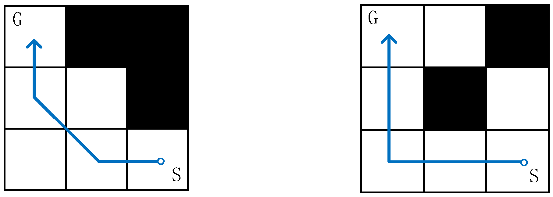
3.3. Optimize Child Node Selection

The storage space of the A* algorithm consists of all the adjacent child nodes around the current point, and the node with the lowest evaluation function is selected as the path node each time. The rule of selecting a child node is to judge whether the child node is a barrier grid; if it is, no child node in this position is generated. Therefore, the planned path may skew over the vertices of obstacles or even over the vertices where two obstacles meet, which may easily lead to collision between the moving machine and obstacles. The risk path is shown in Figure 6.

Figure 7 shows the relationship between the parent node and each child node. The position relationship between the eight child nodes and the parent node is divided into three categories. The two child nodes above and below the parent node (child nodes 2,6) are classified into class Ⅰ, and the two child nodes around the parent node (child nodes 4,8) are classified into class Ⅱ. The remaining four sub-nodes (sub-nodes 1,3,5,7) are divided into class III.

To solve the problem of collision risk in the traditional A* algorithm, this paper adds a child node selection rule to determine the position relationship between child nodes and obstacles when generating child nodes to avoid the path passing diagonally through the obstacle vertex. Taking Figure 7 as an example, when generating the set of child nodes and avoid passing through the vertex of obstacles, assume that a child node is an obstacle, and the child node selection rule is defined as follows:

(1)

When the obstacle child node is in a class I position, the left and right two optional child nodes of the obstacle child node are deleted (such as child nodes 1,3 or child nodes 5,7);

(2)

When the obstacle child node is in a class II position, the two optional child nodes above and below the obstacle child node are deleted (such as child nodes 1,7 or child nodes 3,5).

(3)

When the obstacle child node is in a class III position, it will not be processed.

After the selection rules of the above optimization mode, the path searched by the improved A* algorithm can effectively avoid the risk path, no longer skew over the vertex of the obstacle, and avoid the collision between the mobile robot and the obstacle during movement. The risk path shown in Figure 7 is shown in Figure 8 after optimizing the child node.

3.4. Path Smoothness Optimization

To solve the problem of path smoothness, this paper optimizes the bidirectional smoothness of the calculated path nodes and sets the safe distance between the path nodes and obstacles for anti-collision processing.

In the map constructed by the raster method, the path of operation is composed of several groups of raster center points. The path is not the shortest and the smoothness is low because there are several transitions, and the path nodes can only be in the middle of the grid. This work develops a path smoothness optimization approach for bidirectional junction judgment to address these issues. The middle redundant path nodes of a path node can be removed if there are no obstacles in the way of the connection and the distance between two non-adjacent path nodes is shorter than the planned connection path distance.

In the two-way optimization, the anti-collision isolation distance is increased, and the relationship between the vertical distance from the obstacle point to the line and the set safety distance is used to judge whether the path is safe and realizes anti-collision. The obstacle–isolation relationship is shown in Figure 9. Suppose the coordinates of path node A $(x_a,y_a)$ and B $(x_b,y_b)$ and obstacle point C $(x_c,y_c)$. It is judged that distance CE is the vertical distance of the line segment between obstacle point C and node AB, denoted as $d$. Line segment CD is the distance of the longitudinal axis of the line segment between obstacle point C and node AB, denoted as $l$. The angle between the line segment and the horizontal axis between node AB is denoted as $\alpha$. The side length of the element barrier grid is denoted by $d\text{\_}cell$, and the radius of the external circle is denoted by $r$.

The distance from the obstacle point to the path can be obtained from the coordinates of A, B, and C.

$$l=\left|y_c-(\frac{y_a-y_b}{x_a-x_b}(x_c-x_a)+y_a)\right|$$

(10)

$$\alpha =\left|\mathrm{ractan}\frac{y_a-y_b}{x_a-x_b}\right|$$

(11)

$$d=l\cos \alpha$$

(12)

$$r=d\text{\_}cell/\sqrt{2}$$

(13)

Set the safety distance $D$ (whose value meets $D>r$) for collision isolation. The distance $d$ from the obstacle point to the path is calculated by Formula (12), and the relationship between the distance and the safety distance $D$ is determined as follows:

(1)

If $d\le D$, the path cannot be selected.

(2)

If $d>D$, the path can be selected.

Figure 10 shows the grid path to the graph example. Using the A* algorithm planning path, which is composed of grid nodes, and the diagram before optimization path for S, n1, n2, n3, n4 interchange, n5, n6, n7, n8, n9, n10, and G, there are many paths of redundant nodes, many twists, and problems, such as the path node being limited to being in the grid’s center. The path is not the shortest, and the smoothness is low if the path found by the A* algorithm is immediately inserted into the local dynamic method.

The path nodes operated by the A* algorithm are optimized in this paper through the bidirectional deletion of redundant nodes and obstacle distance judgment. Additionally, bidirectional smoothness optimization increases the smoothness of the path, reduces the number of transition degrees and path length, and opens new options for path node selection beyond the grid’s center. The following are the steps in path smoothness optimization:

Step 1: Only the start, inflection, and finish points should remain in the path node after the intermediate points on the same line are deleted. Figure 10 illustrates the processed path as S→n7→n8→n9→G.

Step 2: From the starting point S direction, take a node every $k$ other step between the two reserved inflection points ni and nj and determine whether there is an obstacle in the path between the two points. Calculate the distance $d$ between the obstacle and the path according to Formula (12), and then determine $d$ and the safe distance $D$ from the path. If the obstacle is beyond the safe distance, the current node is selected as the path node. Otherwise, do not select. As shown in Figure 10, the processed path is S→n11→G.

Step 3: From the direction of the destination location G, take the point judgment in reverse (repeat the step 2 judgment process). The optimum path is S→n12→G, as Figure 10 illustrates. It displays the optimization path. The algorithm comes to an end (Algorithm 1).

Algorithm 1 IA*

Require: Raster map(n), Max(x), Max(y), Start point(S), Target point(T) Ensure: Number of Obstacles(m), Open list = [], Close list = [] 1. map = []/Initializes the environment map matrix 2. k = 1; 3. CLOSED = [] 4. for j = 1: Max(x) 5.  for i = 1: Max(y) 6.   if (Max(i,j) == 1) 7.   plot(i + 5,j + 5, ‘ks’, ‘MarkerFaceClolor’, ‘b’) 8.   fill([i, i + 1, i + 1, i],[j, j, j + 1,j + 1], ’k’;) 9.   CLOSED(k,1) = i 10.   CLOSED(k,2) = j 11.   K = k + 1 12.    else 13.    fill([i, i + 1, i + 1, i],[j, j, j + 1, j + 1], [1, 1, 1]) 14.   end 15.  end 16. end

3.5. Steps to Improve the A* Algorithm

Part of the source code of (Algorithm 1) is shown in the above three-line table. First, initialize the two-dimensional raster map, clear the open list and close list, and then set the obstacle map. Go through each grid and determine whether it is an obstacle grid if it is marked as black; otherwise, it is marked as white.

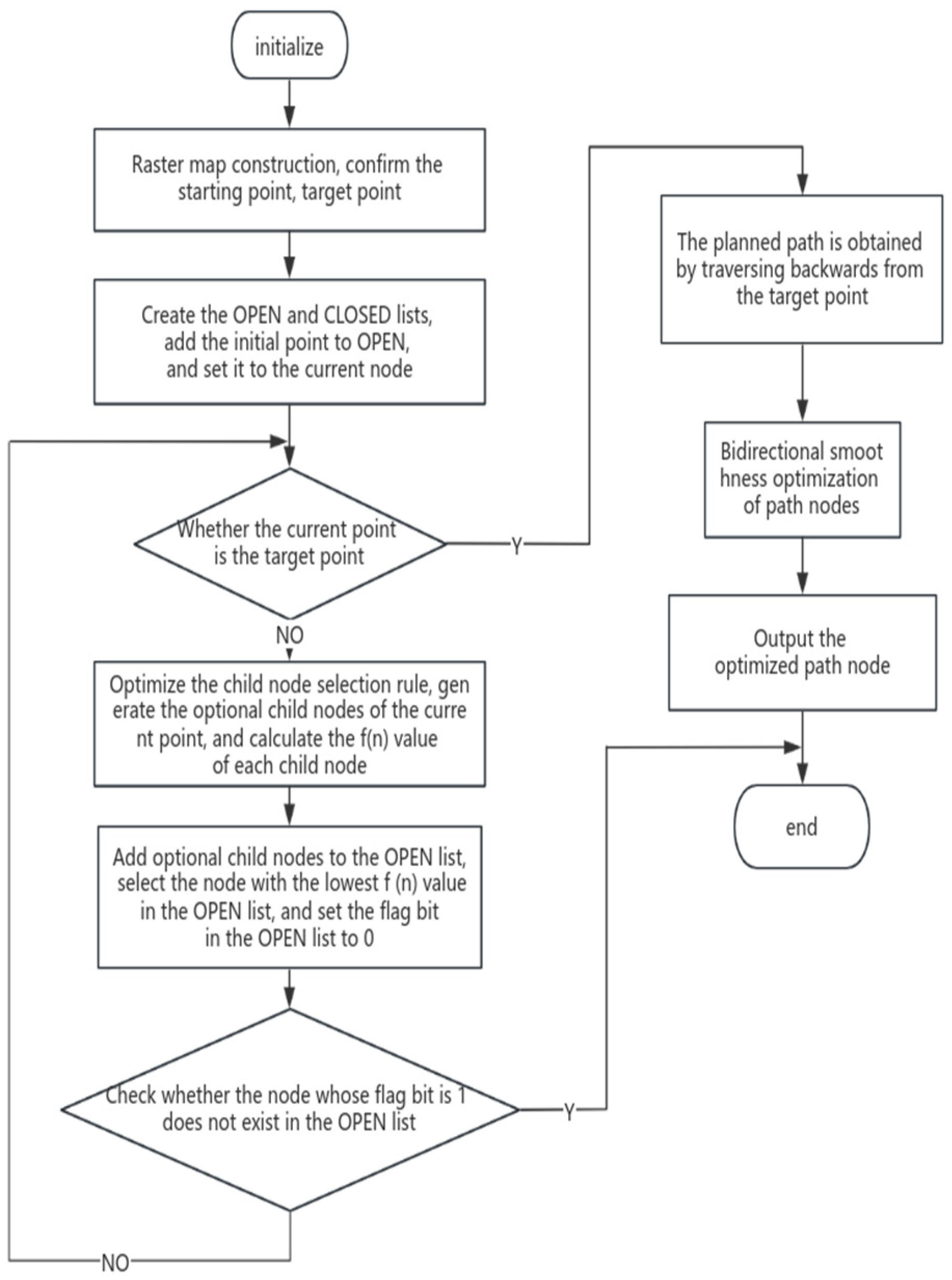
The flowchart of this paper’s single-destination path planning algorithm based on the improved A* algorithm between points is shown in Figure 11.

The steps for improving the A* algorithm designed in this paper are as follows:

Step 1: The grid method is used to model the map environment, and a grid environment of size $x_{\max }\times y_{\max }$ is established. The generated $x_{\max }\times y_{\max }$ rectangle stores the grid state information, and the obstacle rate $P$ is calculated and saved according to Formula (6). Set the robot position coordinate as the starting point and the destination coordinate position as the target point.

Step 2: Establish an open list and a closed list, leave the CLOSED table empty and add the start point to the OPEN table, and set the current point as the start point.

Step 3: Determine whether the current point is the destination. If not, go to Step 4. If so, go to Step 9.

Step 4: Generate eight child nodes of the current point, add child node screening rules, delete the child nodes that have passed the obstacle vertex, and generate optional child nodes.

Step 5: Calculate the cost function $g(n)$, heuristic function $h(n)$, and evaluation function $f(n)$ of each child node, respectively, in Equations (7)–(9).

Step 6: Add the information of the child node (tag bit 1, the coordinate of the child node, the coordinate of the parent node; add value $g(n)$, value $h(n)$, and value $f(n)$ to the open list, select the node with the smallest value $f(n)$, and set its flag bit to 0).

Step 7: Add the smallest node in the $f(n)$ and make it the active node by adding it to the closed list.

Step 8: Determine whether the node marked with bit 1 does not exist. If it does not exist, no node can be selected. The algorithm ends and the operation fails. If yes, go to Step 3.

Step 9: Search the parent node backward from the target point and generate a set of path coordinate arrays from the initial point to the destination.

Step 10: Make a bidirectional connection judgment on the path node, optimize the path node, and generate a new path node array.

Step 11: Output path node array, that is, the search path, and the algorithm ends.

4. Simulation Experiment and Analysis

In the MATLAB environment, the effectiveness of the single-destination routing planning algorithm based on the improved A* algorithm is verified, and some other algorithms and the conventional A* algorithm are contrasted with the enhanced A* algorithm created in this work. Raster map model sizes are 30 × 30 and 50 × 50, respectively. Set the unit raster side length to 1 m in the raster map environment. The moveable region is represented by the white area, while the obstacle is represented by the black area. Point S is the robot’s initial position coordinate or its position coordinate. Point G represents the destination position coordinates, i.e., the target point. The improved A* algorithm parameter take point step is $k$ = 1, and the safety distance is $D$ = 0.8 m.

4.1. Experiment 1: Algorithm Effectiveness Analysis

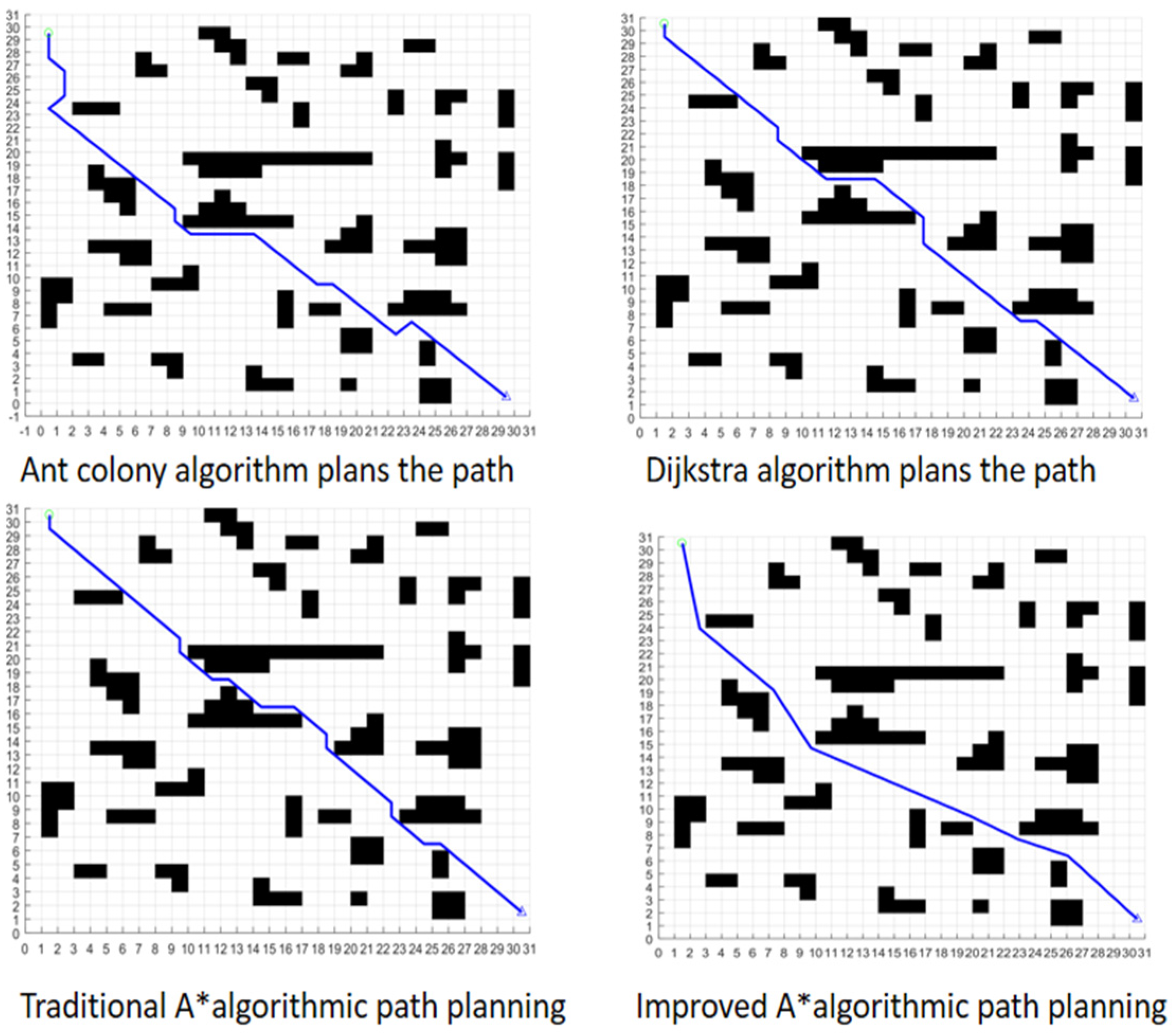
The ACO algorithm, Dijkstra algorithm, traditional A* algorithm, and improved A* algorithm are compared and analyzed, and the performance of each algorithm and the planned path are tested in a 30 × 30 map scale environment. The number of parameter iterations in the ant colony algorithm is 200 times. The paths planned by the ACO algorithm, Dijkstra algorithm, traditional A* algorithm, and improved A* algorithm is shown in Figure 12. The performance data of each algorithm are shown in

Table 1. Performance comparison of the algorithms.

Algorithm	Planning Time (s)	Number of Iterations /Search Space	Path Length (m)	Number of Turns (Times)	Breaking Angle (°)
ACO	188.31	200 iterations	46.77	12	675
Dijkstra	1.26	762 nodes	43.35	9	405
A*	0.93	265 nodes	43.36	13	585
Improved A*	0.91	130 nodes	43.38	6	123

.

As can be seen in Figure 12, the operation path of the ant colony algorithm has a folding path due to the influence of the pheromone level. Dijkstra’s algorithm and the conventional A* algorithm always plan paths that travel toward the goal point; they do not consider the impact of barriers on the path, and the route with the shortest local path is chosen, and there are many turns. The enhanced A* algorithm looks for lower turnover times than conventional algorithms, keeps a safe distance away from obstacles, and avoids collisions with obstacles. After incorporating map information into the heuristics function, it selects an area with fewer obstacles for planning.

From the comparison of experimental data in Table 1, it is evident that the ant colony algorithm requires several iterations to locate ants during path design. In this environment, the maximum number of iterations of the algorithm is set to 200. The experimental results indicate that the iterative search of the ant colony algorithm did not find the optimal path in advance until the last iteration. The path is not the shortest; the number of turns is many. Additionally, the primary method of path planning using the ant colony algorithm is a multi-generation search, resulting in a long operation time. It cannot meet the need for less planning time in multi-destination planning.

When the improved A* algorithm and the traditional A* algorithm search the path, there is heuristic function guidance, the number of path nodes in storage space is less than Dijkstra’s algorithm, and the running time is shorter. This study presents an enhanced A* algorithm that reduces the search space compared to the classical A* algorithm while increasing the guidance of environment information in the evaluation function. The sub-node optimization rules and path smoothness optimization are added so that the running time of the improved A* algorithm is 0.02 s less than that of the traditional A* algorithm, and the difference is not much. However, the planned path has 53.8% fewer turns and 79% fewer turns. Keep a safe distance between the path and the obstacle, making the mobile robot safer.

In a simple environment, although IA* has a slight improvement in time cost compared with A*, in the task processing of robot path planning in a complex environment, the IA* algorithm has achieved a better effect in time cost than the A* algorithm. Twenty experiments have been conducted to compare the results, as shown in

Table 2. Comparison of IA* and A* time cost.

Comparison of ImA* and A* Time Cost
Algorithm	Planning Time	Number of Successful Arrivals
A*	0.2702	18
IA*	0.0993	20

. It can be seen that the IA* algorithm saves a lot of time cost compared with the A* algorithm in complex environments. In two experiments, the A* algorithm failed to find the specified target point in a complex environment, as shown in Figure 13 above. The path planning time in the table is the average time taken to reach the target point for comparison.

4.2. Experiment 2: Algorithm Adaptability Analysis

In order to verify the adaptability of the improved A* algorithm, a simulated indoor environment of obstacles was generated in a 50 × 50 map environment. Five sets of simulation experiments were carried out between the traditional A* algorithm and the improved A* algorithm to test the efficiency and simulation path of the algorithm.

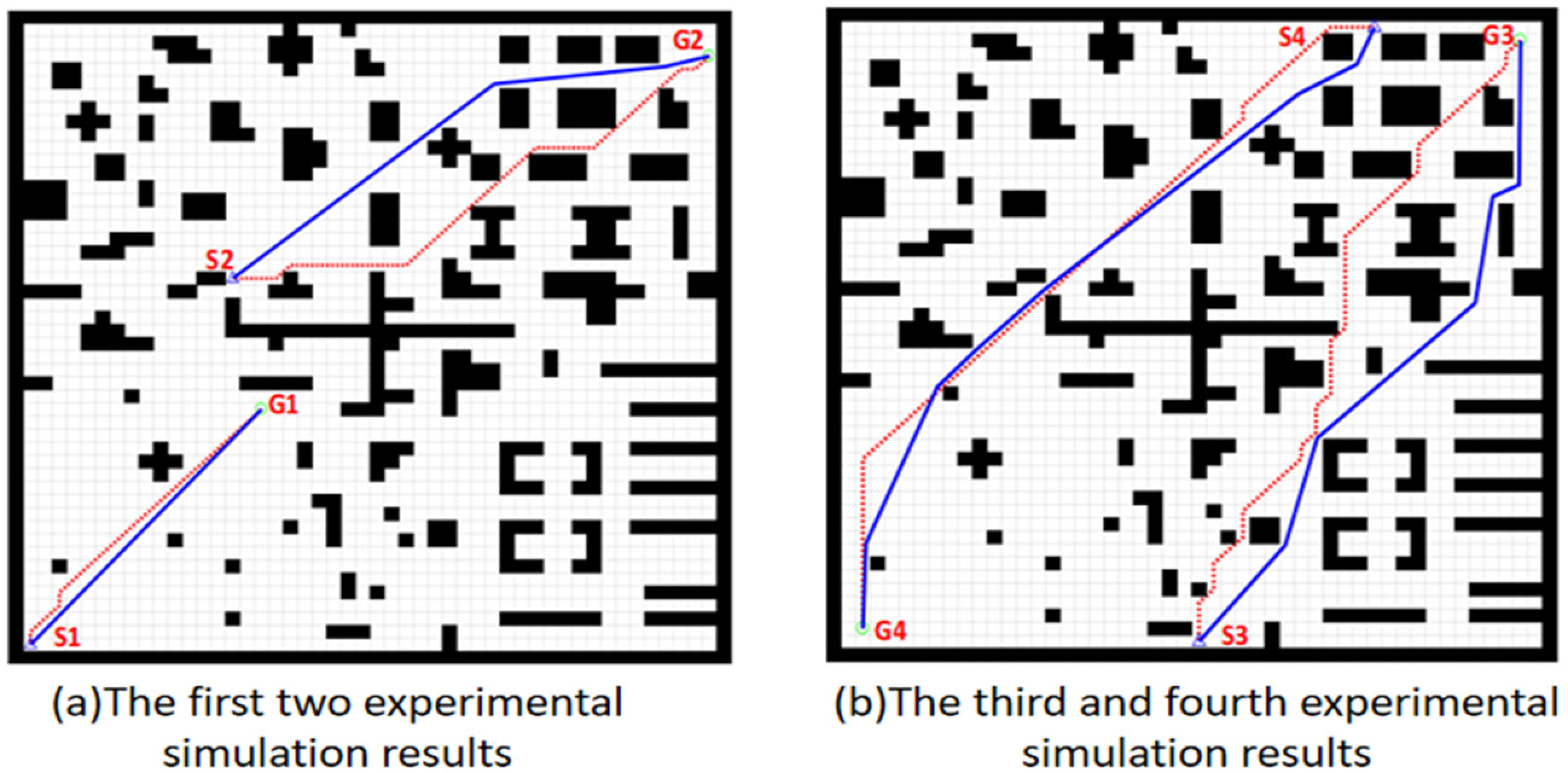
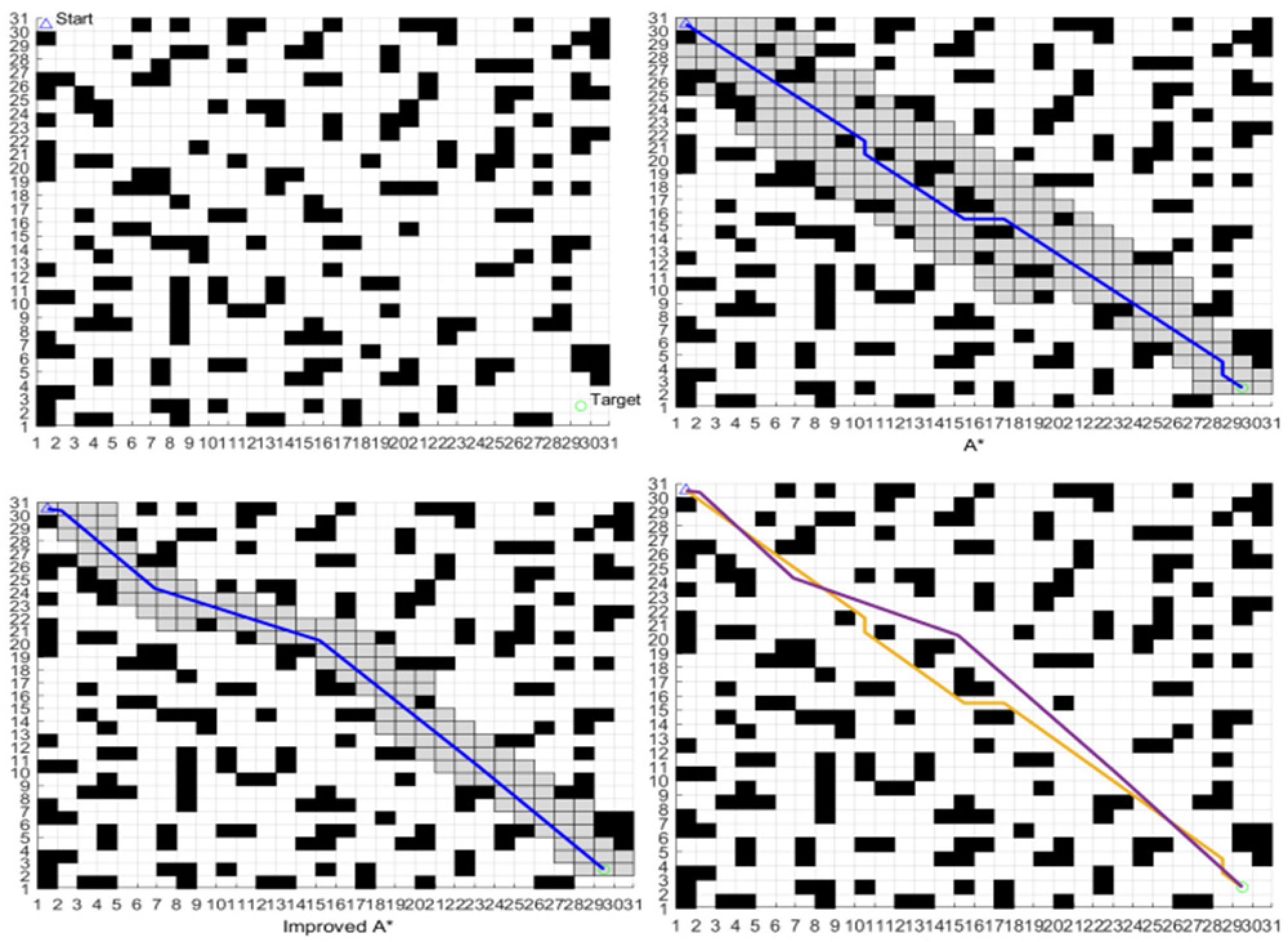
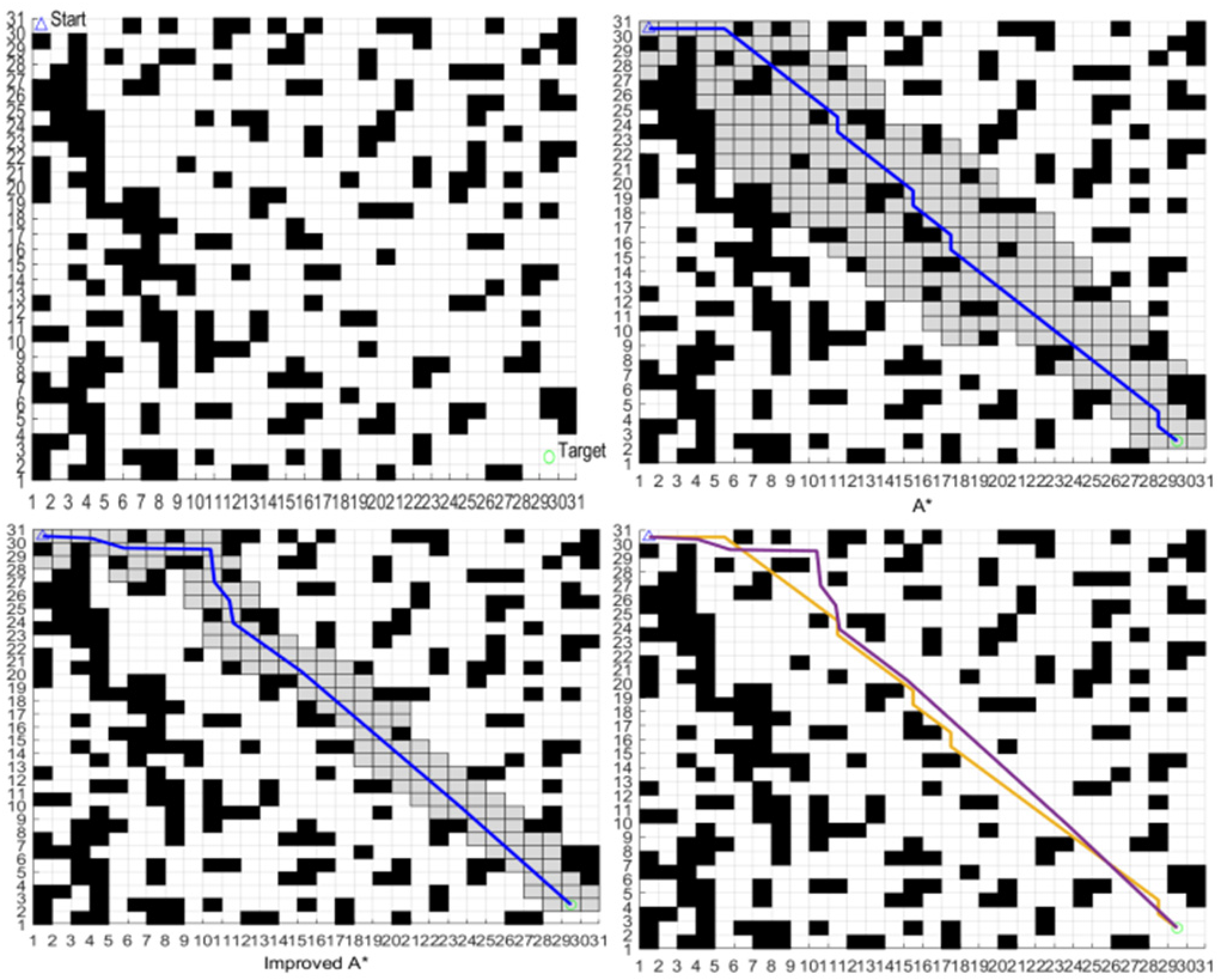
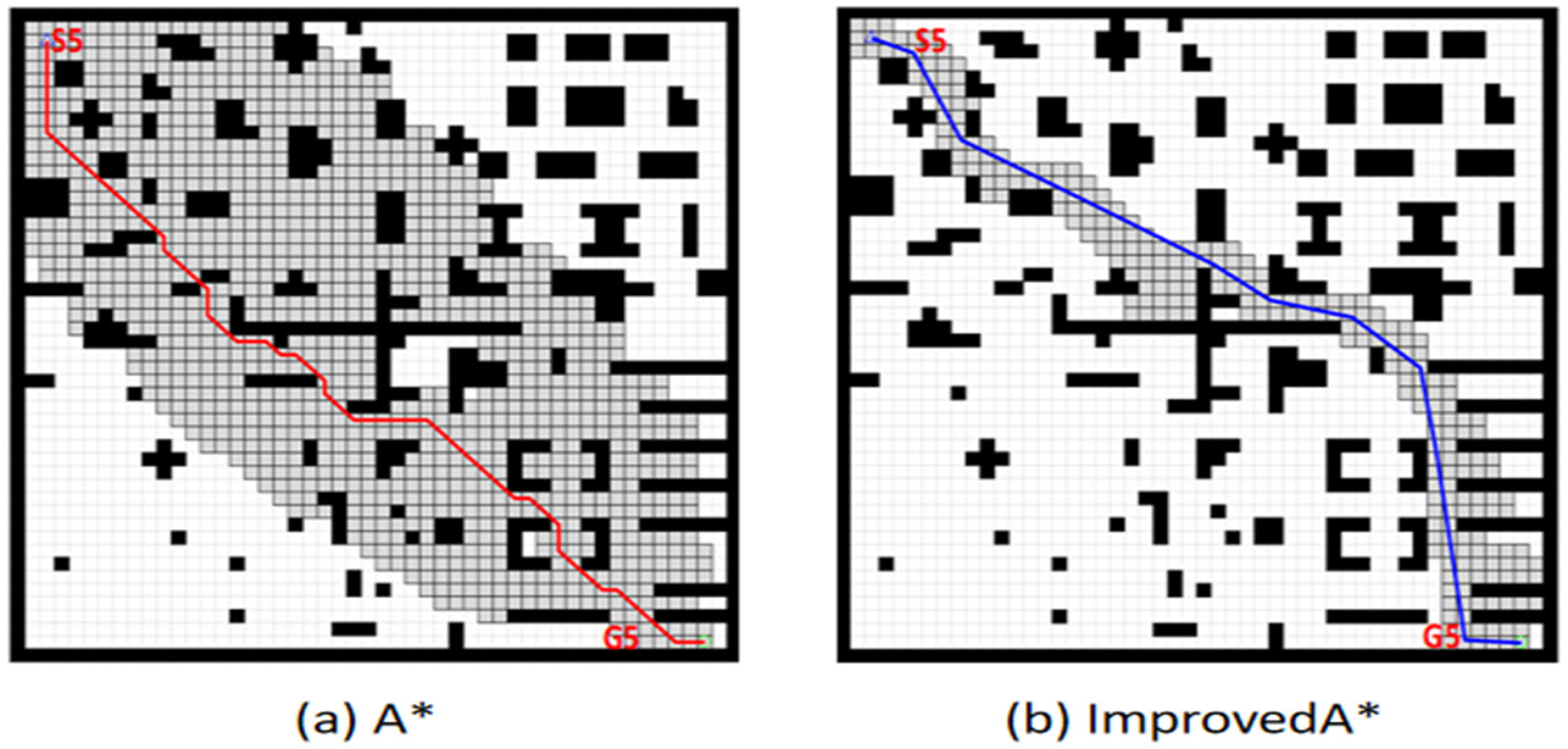
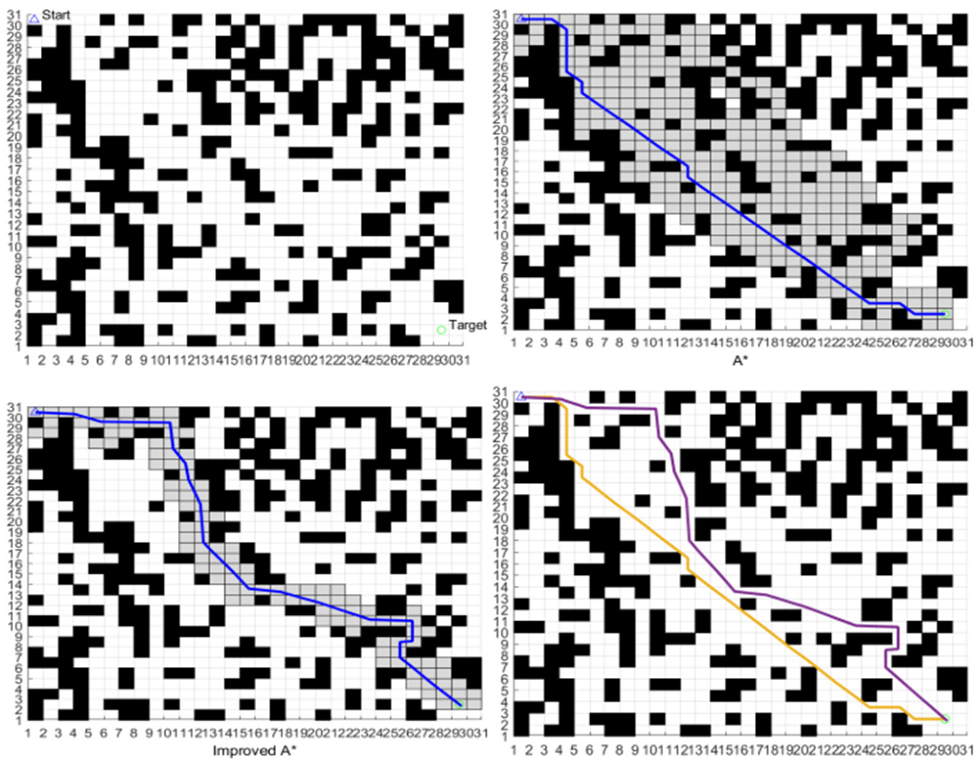
The paths of the five groups of simulation experiments are shown in Figure 14 and Figure 15. In Figure 15, the path planned by the traditional A* algorithm is represented by the red dashed line, and the path planned by the improved A* algorithm is represented by the blue solid line. The gray grid in Figure 15 represents the search space generated by the algorithm, that is, the number of traversing grid nodes.

(S1 G1), (S2 G2), (S3 G3), (S4 G4), and (S5 G5) were the starting and target points of the five groups of experiments.

When there are fewer or more obstacles, the path proposed by the revised A* algorithm is smoother and safer, as seen by the experimental findings in Figure 14 and Figure 15. The number of nodes produced by each algorithm in the search space is displayed in Figure 15.

The conventional A* algorithm reduces the search efficiency of the method by producing a lot of redundant nodes. The enhanced algorithm’s search space is smaller, and its search efficiency is higher.

Table 3. Improved algorithm performance comparison.

Simulation	Starting Point, Target Point	Algorithm	Planning Time (s)	Path Length (m)	Number of Turns (Times)	Breaking Angle (°)	Number of Experiments (Number of Successes)
1st group	(2 2), (18 20)	A*	1.89	24.63	3	135	20 (19)
		I A*	1.72	24.08	0	0	20 (19)
2nd group	(16 30), (49 47)	A*	2.41	40.04	7	315	20 (19)
		I A*	2.03	38.50	2	41.1	20 (19)
3rd group	(26 2), (48 48)	A*	2.79	55.11	17	765	20 (19)
		I A*	2.14	54.18	5	210.9	20 (19)
4th group	(38 49), (3 3)	A*	3.02	62.25	4	180	20 (19)
		I A*	2.64	60.51	6	96.13	20 (19)
5th group	(3 48), (48 2)	A*	3.58	71.67	20	900	20 (19)
		I A*	2.68	71.90	9	253	20 (19)

displays the data of the five groups of simulation experiments, as well as the data analysis of those five groups.

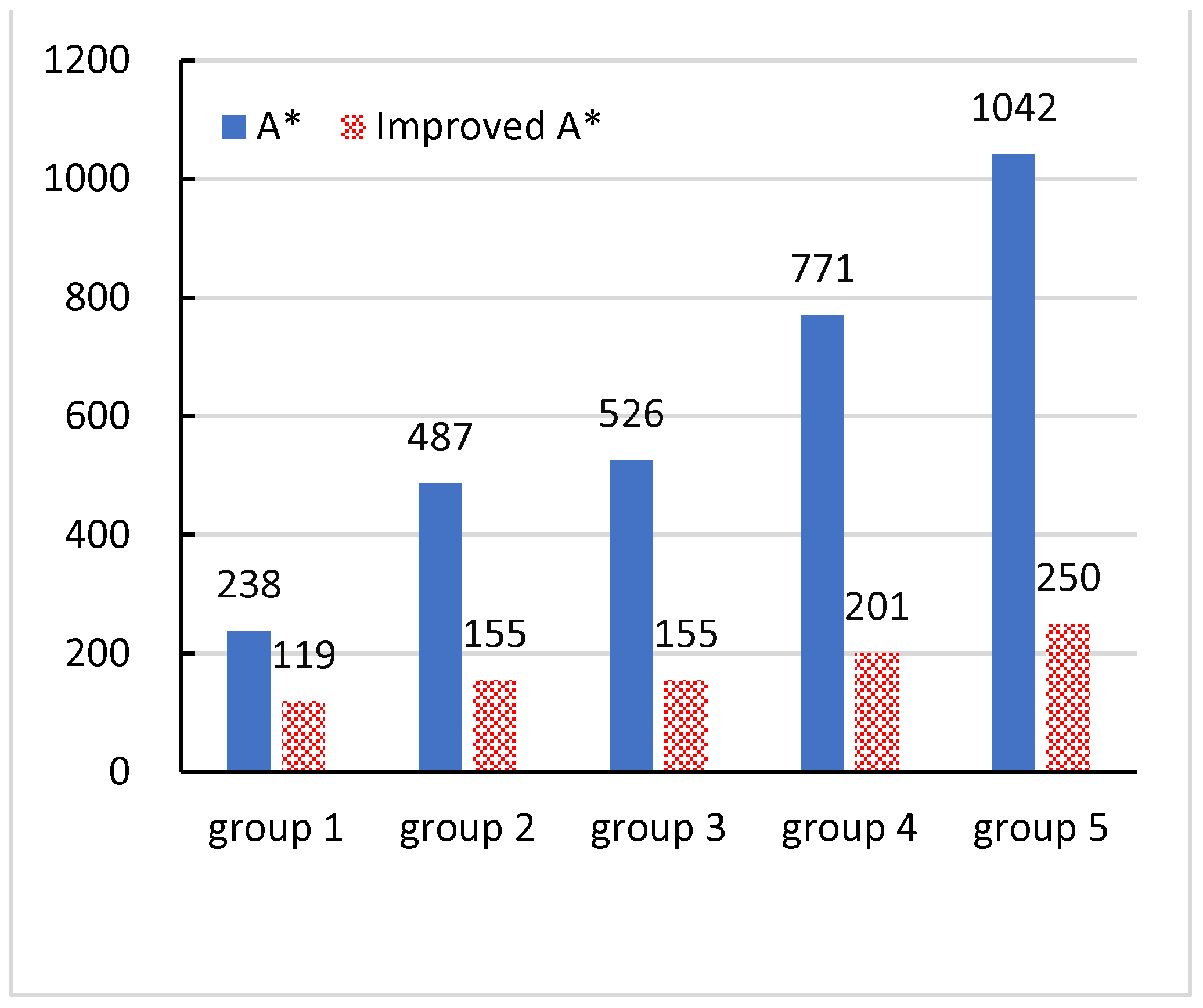
The comparison of the number of nodes in the algorithm search space is shown in Figure 16. As can be seen in the trend of traversing the number of nodes in Figure 16, in raster maps, the enhanced A* algorithm’s efficiency increases with map scale and simulation plan path length. Consequently, bigger storage spaces are required.

The enhanced A* algorithm has a 17.2% reduction in average planning time, a shorter algorithm running time, and a faster algorithm overall. Compared with the traditional A* algorithm, the path length of the improved A* algorithm is reduced by 2.05% on average, and there is little difference between the two algorithms. However, after the improvement of the A* algorithm, there is a 49.4% reduction in the average number of turning points and a 75.5% reduction in the average turning angle. The path planned by the improved A* algorithm is far away from obstacles, and the safety factor is higher. As can be seen in Figure 15, the search space of the improved A* algorithm is reduced by 61.5% on average.

The results of experiment 1 and experiment 2 show that when the planned path with the improved A* algorithm has the same length, the number of deflection angles is reduced, the sum of deflection angles is greatly reduced, and the smoothness of the path is improved. Therefore, when the suggested technique is compared to the conventional A* algorithm, it not only saves storage space and increases search efficiency but also improves the smoothness and security of the path. At the same time, the improved A* algorithm has less operation time for point-to-point single-destination path planning. It is suitable for the requirement of a fast operation rate for multi-destination path planning.

The improved A* algorithm proposed in this paper is compared with the traditional A* algorithm in efficiency, accuracy, and adaptability to complex environments (Figure 17, Figure 18 and Figure 19).

The comparative experiments conducted in this paper define the same starting point and endpoint under raster maps with different complexity levels and take planning time, turning angle, turning number, path length, and traversal node number as performance indicators to measure the differences between the proposed algorithm and the traditional algorithm in efficiency, accuracy, and applicability in complex environments (

Table 4. Comparison of performance indicators in low-complexity environments.

Experiment 1: Complex Environment with Low Complexity
	Planning Time	Degree of Transition	Number of Transitions	Path Length	Number of Traversal Nodes
A*	0.0399	270.00	6	40.77	210
Improved A*	0.0297	92.79	4	40.41	127

,

Table 5. Comparison of performance indicators in medium-complexity environments.

Experiment 2: Complex Environment with Medium Complexity
	Planning Time	Degree of Transition	Number of Transitions	Path Length	Number of Traversal Nodes
A*	0.0569	405	9	41.94	245
Improved A*	0.0303	217.78	8	40.81	128

and

Table 6. Comparison of performance indicators in high-complexity environments.

Experiment 3: Complex Environment with High Complexity
	Planning Time	Degree of Transition	Number of Transitions	Path Length	Number of Traversal Nodes
A*	0.0731	450	10	43.11	286
Improved A*	0.0402	296.74	7	41.12	116

).

Since both algorithms can reach the set target point under different complexity environments, both algorithms have high accuracy and efficiency. As can be seen in Table 4, Table 5 and Table 6, the algorithm proposed in this paper is significantly better than the traditional A* algorithm in terms of planning time under different complexity environments. In terms of applicability, the algorithm proposed in this paper is significantly less in terms of turning angles and times. It can reduce the energy loss of the mobile robot to a greater extent, and the number of traversal nodes is less, which can save the computing memory of the mobile robot.

Compared with the advanced heuristic algorithm and intelligent algorithm in recent years, the results of five experiments are shown in the figure below (Figure 20 and Figure 21).

In the same complex environment, by comparing the time cost and the number of path inflection points between the four algorithms and the IA* algorithm, it can be concluded that the IA* algorithm takes the least time and cost to complete path planning in the environment of the same complexity, and the path experiences the least inflection points, so it can be concluded that the path is relatively smooth, which is beneficial to the mobile robot to efficiently complete the path planning task.

The simulation experiment adopts the classification method, which is robust, comprehensive, and suitable for dealing with some exploratory tasks. The classification method illustrates the working principle of the experiment through three orthogonal dimensions: reproducibility, predictability, and temporality.

The experimental part is divided into three dimensions by classification, which can be explained as follows. 1. The source code can make the experiment reproducible in the same complex environment. 2. In a raster map, when you set the starting point and the target point, the path chosen by the robot is predictable at some nodes due to the setting of the heuristic function. 3. In terms of the time dimension, the introduction of the inspired function obstacle rate P can shorten the exploration time to a certain extent, but if the starting point can be selectively adjusted, the exploration efficiency can be better improved.

5. Conclusions

This paper first introduces the principle of path planning based on the traditional A* algorithm. Then, aiming at the influence of environmental information on path planning, an improved A* algorithm is proposed. The evaluation function incorporates environmental data and optimizes the A* algorithm’s node selection rule, and the goal of the bidirectional smoothness optimization approach is to enhance path smoothness by eliminating unnecessary path nodes. Finally, simulation experiments are carried out in MATLAB, and the simulation results demonstrate that to guarantee the effectiveness of path planning, the algorithm in this study enhances the search mechanism and flexibility of the A* algorithm by efficiently building the search space of the path by the map environment. The algorithm’s flexibility, precision, and search efficiency increased, and the average search space shrunk by 61.5%. The planned path is always away from obstacles to avoid collision. In addition, the number of turning degrees has been reduced by 75.5%, and the smoothness has been greatly improved. The improved A* algorithm takes the least time to plan, and the number of redundant nodes is small, which greatly reduces the search space for the robot, optimizes the selection of child nodes, and optimizes the bidirectional smoothness of the path. All these performance improvements are suitable for the requirements of inspection robots in complex environments. At present, the shortcoming of this algorithm is that it only considers the main problems in this background and proposes optimization solutions, without specific analysis and improvement of corresponding problems in other specific scenarios. Therefore, the algorithm may fail to achieve the expected effect when applied in some specific environments. In addition, the algorithm has obtained optimization results through comparative analysis of several experiments, but it has not been put into practical application, so its robustness when applied to specific robots needs to be tested.