A Production Prediction Model of Tight Gas Well Optimized with a Back Propagation (BP) Neural Network Based on the Sparrow Search Algorithm

Abstract

The production of tight gas wells decreases rapidly, and the traditional method is difficult to accurately predict the production of tight gas wells. At present, intelligent algorithms based on big data have been applied in oil and gas well production prediction, but there are still some technical problems. For example, the traditional error back propagation neural network (BP) still has the problem of finding the local optimal value, resulting in low prediction accuracy. In order to solve this problem, this paper establishes the output prediction method of BP neural network optimized with the sparrow search algorithm (SSA), and optimizes the hyperparameters of BP network such as activation function, training function, hidden layer, and node number based on examples, and constructs a high-precision SSA-BP neural network model. Data from 20 tight gas wells, the SSA-BP neural network model, Hongyuan model, and Arps model are predicted and compared. The results indicate that when the proportion of the predicted data is 20%, the SSA-BP model predicts an average absolute mean percentage error of 20.16%. When the proportion of forecast data is 10% of the total data, the SSA-BP algorithm has high accuracy and high stability. When the proportion of predicted data is 10%, the mean absolute average percentage error is 3.97%, which provides a new method for tight gas well productivity prediction.

1. Introduction

Oil and gas well production prediction is one of the important contents of oil and gas reservoir development scheme design. Predecessors have carried out a lot of research on oil and gas well production prediction, and put forward various production prediction methods. They can be roughly divided into three categories: mechanism model production prediction method, decline curve production prediction method, and intelligent algorithm production prediction method based on big data. A conventional oil reservoir is one that has a stable geological structure, high rock porosity and permeability, and can typically be explored and produced using conventional seismic exploration and drilling technology. An unconventional reservoir, on the other hand, is one that has a complex geological structure and low rock porosity and permeability. This includes shale gas, tight oil, and oil sand, among others. Oil and gas reservoirs frequently necessitate the use of unconventional techniques, such as horizontal wells and fracturing, which are more costly than conventional reservoirs but also have greater potential reserves. In the field of unconventional oil and gas well production prediction, mechanical production prediction models are mostly established based on the double medium theory put forward by Warren and Root [1] in 1963. The dual medium theory assumes that fractured reservoirs are composed of uniformly distributed matrix systems and natural fracture systems. On this basis, many scholars have established the prediction model of tight oil and gas production. The representative scholars comprise Guo et al. [2], Horne et al. [3], Lian et al. [4], Larsen et al. [5], Raghavan et al. [6], Chen et al. [7], Ozkan et al. [8], Yao et al. [9], Su et al. [10], Ren et al. [11,12], Tang [13], and Bai et al. [14]. In 1945, Arps [15] established an exponential decline, hyperbolic decline, and harmonic decline model for predicting oil and gas well production based on the law of oil well decline.

However, most of these models are suitable for the development of conventional oil and gas reservoirs. In order to solve the percolation problem of unconventional oil and gas reservoirs, domestic and foreign scholars have established many production prediction models of decline curve, such as Ilk et al. [16], Valk ó P.P. [17], Duong [18], and Hong [19]. The prediction of production and reserves of tight oil and gas reservoir is an important part of reservoir engineering, and also a key index to evaluate the development effect of oil and gas field. Multi-stage fractured horizontal well technology is used to develop unconventional oil and gas reservoirs. The complexity of fluids near reservoirs and production wells makes conventional production decline method, such as the Arps production decline method, not applicable in many cases. At present, most of the models used to predict production and reserves of production wells are analytical, numerical, or empirical models. In contrast, the empirical model (production decline method) is still the most widely used method in the oil and gas industry to predict future production and reserves based on dynamic production trends. It is simple, easy to operate, has good time-to-production, and allows us to easily predict production and life cycles. The actual application shows the following: (1) The longer the production time and more data used in forecasting, the smaller the relative error, but when the data of the first year are included, it is easy to underestimate the output. (2) SEPD, YM-SEPD, and Duong are more suitable for early decline, while hyperbolism is suitable for late decline. The production data predicted by the late SEPD model are often low, while the value predicted by the Duong model is high. Therefore, the combination model is recommended for the analysis of tight oil and gas production decline. (3) Select wells with a long production history and analyze the time for a single well to reach the boundary control flow. When the production time is less than this time, the comprehensive use of YM-SEPD method and Duong method can obtain conservative and reliable results; after the boundary effect appears, the hyperbolic decline method is more convenient to predict than other methods.

However, the above two kinds of methods are established on the basis of certain assumptions and cannot 100% reflect the law of real formation seepage. In order to solve the defects of traditional prediction methods, scholars introduce machine learning technology into the field of oil and gas exploration and production. The random forest algorithm, support vector machine, artificial neural network, and other technologies are applied in the field of productivity prediction. Scholars have established the production prediction model of oil and gas wells based on artificial neural networks. In 2008, Ni [20] and others used artificial neural network to predict productivity and establish a three-layer BP neural network model, but the network will have the problem of slow convergence and low accuracy. In order to improve the convergence speed, in 2011, Li [21] adopted the Lmure M (Levenberg–Marquardt) algorithm to optimize the loss function on the basis of BP neural network to accelerate convergence, but the problem of low convergence accuracy still appeared without optimizing the weights and thresholds of the network. In 2015, Ma [22] used genetic algorithm to optimize the BP neural network to optimize the network weight, but the neural network will still converge slowly and fall into local optimization in the highly volatile data. However, the above two kinds of methods are established on the basis of certain assumptions and cannot fully (100%) reflect the law of real formation seepage. In order to solve the defects of traditional prediction methods, scholars introduce machine learning technology into the field of oil and gas exploration and production.

In order to solve the problems of slow convergence and susceptibility to local optima the BP neural network, this paper optimizes the activation function and loss function of the BP neural network, and then uses the sparrow search algorithm to optimize the weight and threshold of the BP network. On this basis, the SSA-BP neural network’s productivity prediction model is established, which provides a good prediction tool for calculating the production of tight gas wells.

2. Principle of Sparrow Search Algorithm

The sparrow search algorithm (SSA) was proposed by Xue [23] in 2020. The SSA mainly imitates the foraging behavior and anti-predation behavior of sparrows. The whole process is a mechanism in which the participant follows the discoverer and superimposes vigilant at the same time. Discoverers often have a better adaptation value, can find a better foraging location, and explore a wide range. In order to improve their fitness, the participants always look for food around the discoverers, while the participators may constantly monitor the discoverers and compete for food sources in order to increase their predation rate. At the same time, the sparrow population will randomly appear a certain proportion of vigilant; when the danger is found, the alarm will be issued by the discoverer to decide whether to anti-feeding. With each iteration, the discoverer location is updated, as follows:

$$X_{i,j}^{t+1}=\left\{\begin{array}{l}{X}_{i,j}.\exp \left(-\frac{i}{\alpha .ite{r}_{\max }}\right),if R_2<S_T\\ X_{i,j}+Q.L,if R_2\ge S_T\end{array}\right.$$

(1)

where t represents the current number of iterations, iter_max 1 and 2, 3, …, d. ${inter}_{\max }$ is a constant that represents the maximum number of iterations. $X_{ij}$ represents the location information of the Ist sparrow in dimension j. $\alpha \in \left(0,1\right]$ is a random number; $R_2\left(R_2\in \left[0,1\right]\right)$ and $S_T\left(S_T\in \left[0.5,1\right]\right)$ denote early warning value and safety value, respectively. Q is a random number with a normal distribution. L denotes a 1 × d matrix, where each element in the matrix is 1.

When $R_2<S_T$, this means that there are no predators around the foraging environment, and the discoverer can perform a wide range of search operations. If $R_2\ge S_T$, it means that some sparrows in the population have found predators and have alerted other sparrows in the population, and all sparrows need to fly quickly to other safe places to look for food.

The location of the participant for each iteration is updated as follows:

$$X_{i,j}^{t+1}=\left\{\begin{array}{l}Q.\exp \left(\frac{X_{worst}-X_{i,j}^t}{i2}\right),\hspace{1em}\hspace{1em} if i>\raisebox{1ex}{$n$}\!\left/ \!\raisebox{-1ex}{$2$}\right.\\ X_P^{t+1}+\left|X_{i,j}-X_P^{t+1}\right|\cdot A^{+}\cdot L, otherwise\end{array}\right.$$

(2)

Among them, $X_p$ is the best position occupied by the discoverer at present, and $X_{worst}$ represents the worst position in the whole world. A represents a 1 × d matrix, where each element is randomly assigned to 1 or −1, and $A^{+}=A^T{\left(A{A}^T\right)}^{-1}$. When $i>n/2$, this shows that the i participant with lower fitness value has no food and is very hungry, so it needs to fly to other places to find food in order to get more energy.

The positions of the vigilantes are as follows:

$$X_{i,j}^{t+1}=\left\{\begin{array}{l}{X}_{best}^t+\beta .\left|X_{i,j}^t-X_{best}^t\right|, if f_i>f_g\\ X_{i,j}^t+K.\left(\frac{\left|X_{i,j}^t-X_{worst}^t\right|}{\left(f_i-f_w\right)+\epsilon }\right), if f_i=f_g\end{array}\right.$$

(3)

where is the current global optimal location. As a step size control parameter, $\beta$ is a random number with a normal distribution with a mean of 0 and a variance of 1. $K\in \left[-1,1\right]$ is a random number, and $f_i$ is the fitness value of the current sparrow. $f_g$ and $f_w$ are the current global best and worst adaptation values, respectively. The constant of $\epsilon$ to avoid zero denominator. For simplicity, when $f_i>f_g$ indicates that the sparrow is on the edge of the population, it is extremely vulnerable to predators. $X_{best}$ says the sparrows in this position are the best and are safe in the population. When $f_i=f_g$, this indicates that sparrows in the middle of the population are aware of the danger and need to be close to their sparrows to minimize their risk of predation. K indicates that the direction in which the sparrow moves is also a step size control parameter.

3. Sparrow Search Algorithm to Optimize BP Neural Network

According to the calculation logic of a traditional BP neural network, it is evident that the subject has a strong self-learning ability and non-linear mapping ability, which are very consistent with oil field production prediction. However, when the objective function is very complex, because the loss function in BP algorithm is optimized by gradient descent, it may fall into the trap of local optimization. Moreover, the uncertainty of the network also increases because of the random initialization of weights and thresholds, that is, the weights and thresholds of the network depend on the quality of sample data, which reduces the accuracy of BP neural network in oil field production prediction.

The global search ability of the sparrow search algorithm can better search the weights and thresholds of the BP neural network, so that the neural network can reach a stable state more quickly and obtain the optimal prediction result. The sparrow search algorithm is used to optimize the BP neural network and also to fully utilize their respective strengths, achieving mutual complementarity and improving the accuracy of the model.

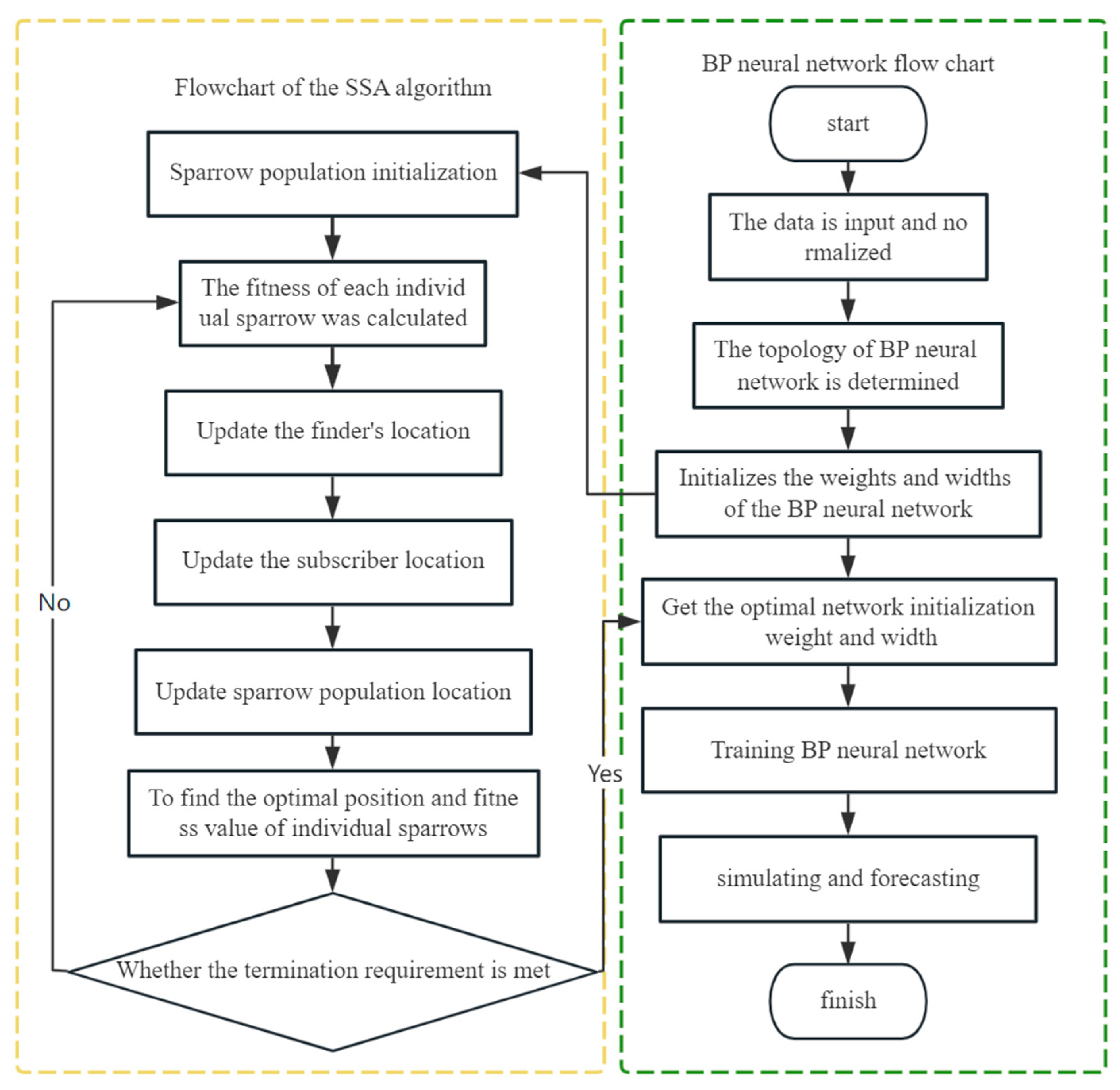
The process of optimizing the BP network via the sparrow search algorithm mainly consists of two parts: sparrow search algorithm optimization and neural network prediction. In order to optimize the sparrow search algorithm, we first determine the sparrow population. Because the weight and threshold are m × n-dimensional matrix, respectively, the vector exists in the BP neural network structure (net). In order to optimize each element, we first take out the elements, and then put them into the vector according to the order to complete the composition of the sparrow population. The length of each sparrow in the population is the sum of all connection weights and threshold lengths of the neural network. There are n neurons in the hidden layer, h neurons in the output layer, w is the weight between the input layer and the hidden layer, lw is the weight between the output layer and the hidden layer, b is the threshold of the hidden layer, and o is the threshold of the output layer. When the input layer is i, the length of the sparrow is I × n + n + n × h + h. The optimization process represented with a flow chart added via the sparrow search algorithm to optimize the BP neural network is shown in Figure 1.

The individual fitness value of the sparrow was calculated. The initial weight and threshold are used for network training, and the overall mean square error (MSE) of the training set and the test set is taken as the fitness function. The smaller the fitness function value is, the more accurate the training is. The sparrow position is gradually updated and iterated to find the global optimal solution, that is, the optimal sparrow individual. The optimal individual position of the output is used as the weight and threshold of the neural network for training and prediction.

4. Case Prediction

4.1. Model Evaluation Criteria

The root mean square error (RMSE), mean absolute error (MAE), and mean absolute percentage error (MAPE) are selected as the evaluation index of the model. The first performance index is the root mean square error (RMSE), which is used to measure the deviation between the predicted value and the actual value. The smaller the root mean square error, the higher the prediction accuracy. The second performance index is the mean absolute error (MAE), which is the average of the absolute error between the predicted value and the actual value, which can directly reflect the actual situation of the predicted error. The closer the value is to 0, the more accurate the prediction. The third performance indicator is the mean absolute percentage error (MAPE), which refers to the ratio of the absolute value of all predicted errors to the actual value. The closer the value is to 0, the more accurate the prediction.

4.2. Neural Network Hyperparameter Optimization

Taking a well (Well-1) in the Ordos Basin as an example, this paper introduces the super-parameter optimization process of activation function, training function, and hidden layers in a BP neural network, and then constructs the SSA-BP network model. Among them, the data of more than 600 days since the production of Well-1 are taken as a sample, and the predicted data accounts for 10%. The four nodes in the input layer of the neural network are cumulative production time, daily production time of the gas well, oil pressure, and casing pressure.

(1)

Optimization of activation function

The predicted values of the BP neural network under different activation functions are shown in

Table 1. Forecast error table under different activation functions.

Activation Function	Logsid	Tansig	Purelin
Mean absolute error (MAE)	1.2601	0.70203	1.2872
Mean square error (MSE)	1.6058	0.52161	1.7083
Root mean square error (RMSE)	1.2672	0.72223	1.307
Mean absolute percentage error (MAPE)	26.87%	14.93%	27.41%

. It can be seen that the hyperbolic tangent S-type transfer function (tansig) is the best for the input layer activation function, so the activation function is tansig.

(2)

Optimization of training function

When the activation function is tansig, the prediction accuracy of the BP network under different training functions is shown in

Table 2. Forecast error table under different training functions.

Training Function	Traingd	Trainrp	Trainbfg	Trainlm
Mean absolute error (MAE)	1.0102	2.2183	0.67071	0.44247
Mean square error (MSE)	1.0517	5.7882	0.46471	0.20631
Root mean square error (RMSE)	1.0255	2.4059	0.6817	0.45422
Mean absolute percentage error (MAPE)	21.59%	47.56%	14.33%	9.37%

; it can be seen that the prediction effect is the best when the training function is trainlm (Lmurm algorithm), so the training function is optimized for trainlm.

(3)

Optimization of the number of hidden layers and nodes

The single hidden layer BP neural network model and the double hidden layer neural network model are established, respectively. The number of hidden layer neuron nodes is adjusted using the following empirical formula.

$$hiddennum=\sqrt{m+n}+a$$

(4)

In the formula, m is the number of nodes in the input layer, n is the number of nodes in the output layer, and a is generally taken as an integer between 1 and 10.

The number of hidden layer neurons in the single hidden layer network model is 7. In the double hidden layer neural network model, the best number of nodes in the first hidden layer is 9, and the best number of nodes in the second hidden layer is 5. The prediction results of the model are shown in

Table 3. Forecast error table under different hidden layers.

Evaluation Criteria	Double Hidden Layer	Single Hidden Layer
Mean absolute error (MAE)	0.36743	0.70203
Mean square error (MSE)	0.14877	0.52161
Root mean square error (RMSE)	0.3857	0.72223
Mean absolute percentage error (MAPE)	7.77%	14.93%

, and the results show that the prediction effect of double hidden layers is better.

(4)

SSA-optimized BP neural network model

On this basis, SSA is used to optimize a single-layer BP neural network and double-layer BP neural network, respectively. The population size of the sparrow algorithm is set to 30, the maximum evolution algebra of population is 50, the proportion of discoverers is set to 70%, and the proportion of vigilant is set to 20%. The best sparrow individual is optimized with the sparrow search algorithm, which is used as the weight and threshold of the BP neural network. Results as shown in

Table 4. Forecast error table under different hidden layers after SSA optimization.

Evaluation Criteria.	SSA—Double Layer BP	SSA—Single Layer BP
Mean absolute error (MAE)	0.21993	0.17476
Mean square error (MSE)	0.06234	0.036954
Root mean square error (RMSE)	0.24968	0.19223
Mean absolute percentage error (MAPE)	4.60%	3.76%

; after the SSA optimization of weights and thresholds, the prediction effect of single hidden layer BP network model is better than that of double hidden layer model, and the double hidden layer model will appear to be over-fitting after optimization. Tight gas reservoirs account for more than half of unconventional natural gas resources in China and have a good development prospect. The efficient development of tight gas reservoirs has long-term strategic significance for ensuring energy supply and promoting social and economic development of our country. Due to the special geological characteristics and complex percolation mechanism, tight gas reservoirs are different from conventional gas reservoirs with poor reservoir physical properties, low natural productivity, rapid production decline, and poor production stability, and they usually require horizontal wells and hydraulic fracturing to achieve industrial gas flow. Therefore, it is of great theoretical and practical significance to study the basic seepage theory of different well types of tight gas reservoirs and reveal the influence of various gas well and formation parameters on the development of tight gas reservoirs. This is important in order to accurately grasp the production performance of gas wells and guide the reasonable development of tight gas reservoirs.

Using the single-layer BP model optimized with the sparrow search algorithm and the model without the sparrow search algorithm, the prediction effect of gas well productivity is shown in Figure 2. From Figure 2b, we can see that the network model optimized without the sparrow search algorithm has a poor fitting result in the training stage, and the predicted value of the model in the learning stage is generally lower than the real production value. This is because the selection of weights and thresholds of the model without SSA optimization is random; even if other super parameters of this model have been optimized, it is still difficult to use directly. The model optimized with the sparrow algorithm is obviously better in both the fitting effect of the training section and the test results of the test section (as shown in Figure 2b).

4.3. Comparative Analysis of Prediction Results

In order to further verify the practicability and stability of the SSA-BP neural network built in this paper, the SSA-BP neural network, HongYuan model [20], and Arps model [16] are used to predict productivity based on the actual production data of 20 tight gas wells in the Ordos Basin. The average prediction days are 49.75 days when the forecast accounts for 10%, and the average absolute mean percentage error predicted with the SSA-BP model is 3.97%. The average absolute mean percentage error predicted with the HongYuan model is 33.04%. The average absolute mean percentage error predicted with the Arps model is 22.94%. When the forecast ratio is 20%, the average prediction days are 99.5 days, and the average absolute mean percentage error predicted with the SSA-BP model is 20.16%, indicating that the long-term prediction effect is poor. The average prediction days are 49.75 days when the forecast accounts for 10%, and the average absolute mean percentage error predicted with SSA-BP model is 3.97%. The average absolute mean percentage error predicted with the HongYuan model is 33.04%. The unsteady seepage flow model of the horizontal well in tight gas reservoir is established, and the Pedrosa substitution and regular perturbation theory combined with the Laplace transform, orthogonal transform, and Green’s function theory are applied to solve the model. Additionally, the pressure solution and constant pressure production solution of horizontal well are obtained. The flow stages of uniform medium pressure dynamic and production decline curve can be divided into the pure wellbore accumulation effect stage, transitional flow stage after wellbore accumulation, early vertical radial flow stage, middle linear flow stage, and late system quasi-radial flow stage. The flow stages of the dual medium pressure dynamics and production decline curves can be divided into the pure wellbore accumulation effect stage, transitional flow stage after wellbore accumulation, early vertical radial flow stage, early linear flow stage in fracture system, middle radial flow stage in fracture system, cross-flow stage in matrix system to fracture system, and late quasi-radial flow stage in system. The unsteady seepage flow model of fractured horizontal wells in tight gas reservoirs was established, and the linear sum solution expression was derived by applying Pedrosa substitution, regular perturbation theory, Laplace transform, and Green’s function theory. Then, the pressure solution and constant pressure production solution of fractured horizontal wells were obtained with a discrete analysis of fractured fractures. Hence, the flow stages of uniform medium pressure dynamics and production decline curves can be divided into the pure wellbore accumulation effect stage, transition flow stage after wellbore accumulation perpendicular to the fracturing fracture in the early linear flow stage, near the fracturing fracture in the middle stage of the system linear flow stage perpendicular to the horizontal wellbore, and the late system quasi-radial flow stage. The flow stages of the dual medium pressure dynamics and production decline curves can be divided into the pure wellbore reservoir effect stage, transitional flow stage after concurrent reservoir, fracture linear flow stage, fracture radial flow stage, natural fracture linear flow stage, natural fracture radial flow stage, matrix system to fracture system cross-flow stage, and late total system pseudo-radial flow stage.

5. Conclusions

(1)

This paper optimizes the BP neural network based on the sparrow search algorithm. Aiming at the optimization of the trasig activation function, trainlm training function, and single-layer BP neural network for tight gas wells in the Ordos Basin, the parameters of the sparrow search algorithm are also mentioned, which realizes the automatic optimization of a neural network’s weight and threshold, and avoids the tedious parameter adjustment process of a conventional neural network.

(2)

The production of 20 tight gas wells in the Ordos Basin is predicted by using the SSA-BP neural network, HongYuan model, and Arps model. The results show that the average absolute mean percentage error of the SSA-BP neural network is only 3.97%, the error of the HongYuan model is 33.04%, and the error of the Arps model is 22.94%. It shows that the model established in this paper has high prediction accuracy and can effectively predict the production of tight gas wells.

(3)

The prediction results of the SSA-BP neural network under different proportions of prediction data are compared and analyzed. The average error is 3.97% when the proportion of prediction data is 10%, and the average error is 20.16% when the proportion of prediction data is 20%. The prediction accuracy of the model decreases with the increase in the proportion of prediction data.

References

- Warren, J.E.; Root, P.J. The Behavior of Naturally Fractured Reservoirs. Soc. Pet. Eng. J. 1963, 3, 245–255. [Google Scholar] [CrossRef]
- Guo, G.; Evans, R.D. Pressure-Transient Behavior and Inflow Performance of Horizontal Wells Intersecting Discrete Fractures. In Proceedings of the SPE Annual Technical Conference and Exhibition, Houston, TX, USA, 3–6 October 1993; Paper SPE. p. 26446. [Google Scholar]
- Horne, R.N.; Temeng, K.O. Relative Productivities and Pressure Transient Modeling of Horizontal Wells with Multiple Fractrues. In Proceedings of the SPE Middle East Oil and Gas Show and Conference, Manama, Bahrain, 12–15 March 1995; Paper SPE. p. 29891. [Google Scholar]
- Lian, P.; Cheng, L.; Cao, R.; Huang, S. Unsteady model of coupling between horizontal wellbore and reservoir in low permeability reservoir. Comput. Phys. 2010, 27, 203–210. [Google Scholar]
- Larsen, L.; Hegre, T.M. Pressure transient analysis of multifractured horizontal wells. In Proceedings of the SPE Annual Technical Conference and Exhibition, New Orleans, LA, USA, 25–28 September 1994. [Google Scholar]
- Raghavan, R.S.; Chen, C.C.; Agarwal, B. An analysis of horizontal wells intercepted by multiple fractures. SPE J. 1997, 2, 235–245. [Google Scholar] [CrossRef]
- Chen, C.C.; Rajagopal, R. A multiply-fractured horizontal well in a rectangular drainage region. SPE J. 1997, 2, 455–465. [Google Scholar] [CrossRef]
- Ozkan, E.; Brown, M.; Raghavan, R.; Kazemi, H. Comparison of fractured horizontal-well performance in conventional and unconventional reservoirs. In Proceedings of the SPE Western Regional Meeting, San Jose, CA, USA, 24–26 March 2009. [Google Scholar]
- Yao, J.; Liu, P.; Wu, M. Well test analysis of fractured horizontal well in fractured reservoir. J. China Univ. Pet. 2013, 37, 107–113. [Google Scholar]
- Su, Y.; Wang, W.; Zhou, S.; Li, X.; Mu, L.; Lu, M. Trilinear flow model and fracture arrangement of volume-fractured horizontal well. Sheng Guanglong Oil Gas Geol. 2014, 35, 435–440. [Google Scholar]
- Ren, Z.; Wang, X.; Cui, S.; Yang, X.; Yang, Q.; Bi, G. Semi-analytical percolation model of volume fracturing horizontal well in tight reservoir. Fault Block Oil Gas Fields 2018, 25, 488–492. [Google Scholar]
- Ren, Z.; Wu, X.; He, X.; Li, J.; Zuo, Y.; Lou, E. Unsteady pressure model of inclined fractured horizontal well in anisotropic reservoir. Fault Block Oil Gas Field 2017, 24, 74–78. [Google Scholar]
- Tang, S. Research on Productivity Prediction of Fractured Horizontal Wells in Tight Gas Reservoirs Based on Time Series Method. Master’s Thesis, Xi’an Shiyou University, Xi’an, China, 2023. [Google Scholar]
- Bai, H.; Feng, T.; Du, K.; Wang, Q. Gas well production allocation method based on BP neural network. Chin. Sci. Technol. Pap. 2023, 18, 1000–1006. [Google Scholar]
- Arps, J.J. Analysis of Decline Curves. Trans. AIME 1945, 160, 228–247. [Google Scholar] [CrossRef]
- Ilk, D.; Perego, A.D.; Rushing, J.A.; Blasingame, T.A. Hyperbolic Decline in Tight Gas Sands-Understanding the Origin and Implications for Reserve Estimates Using Arps’ Decline Curves. In Proceedings of the SPE Annual Technical Conference and Exhibition, Denver, CO, USA, 21–24 September 2008. Paper SPE116731. [Google Scholar]
- Valkó, P.P.; Lee, W.J. A better way to forecast production from unconventional gas wells. In Proceedings of the SPE Annual Technical Conference and Exhibition, Florence, Italy, 20–22 September 2010; pp. 19–22, Paper SPE 134231. [Google Scholar]
- Duong, A.N. Rate-decline analysis for fracture-dominated shale reservoirs. SPE Reserv. Eval. Eng. 2011, 14, 377. [Google Scholar] [CrossRef]
- Yuan, H.; Soar, L.; Packer, R.; Bhuiyan, M.; Xu, J. A Case Study to Evaluate Shale Oil Production Performance Models with Actual Well Production Data. In Proceedings of the SPE Unconventional Resources Technology Conference, Denver, CO, USA, 12–14 August 2013. Paper SPE 1582234. [Google Scholar]
- Ni, H.; Wang, W.; Luo, S. Application of artificial neural network in oil production prediction. J. Shaanxi Inst. Technol. (Nat. Sci. Ed.) 2008, 21, 37–40. [Google Scholar]
- Li, C.; Tan, M.; Zhang, K. Study on oil well production prediction based on improved BP neural network. Sci. Technol. Eng. Process 2011, 11, 7766–7769. [Google Scholar]
- Ma, L.; Li, D.; Guo, H.; Li, W. Application of optimizing BP neural network based on genetic algorithm in crude oil production prediction: Taking BED test area of Daqing Oilfield as an example. Pract. Underst. Math. 2015, 45, 117–128. [Google Scholar]
- Xue, J.; Shen, B. A novel swarm intelligence optimization approach: Sparrow search algorithm. Syst. Sci. Control Eng. Open Access J. 2020, 8, 22–34. [Google Scholar] [CrossRef]