1. Introduction
The global demand for energy has been steadily increasing over the last few decades, leading to substantial growth in electricity production worldwide [
1]. Traditionally, conventional fossil fuels have served as the primary energy source for electricity generation. However, the sustainability of these traditional fossil fuel resources is now uncertain due to their rapid depletion [
2]. Moreover, the combustion of fossil fuels is a major contributor to greenhouse gas emissions, exacerbating severe global warming and posing a threat to the planet’s health [
1,
3].
In response to these challenges, there has been a significant shift in focus from fossil fuels to renewable energy sources (RESs) for electricity generation. This transition involves harnessing solar energy, wind energy, tidal energy, and biomass energy [
4,
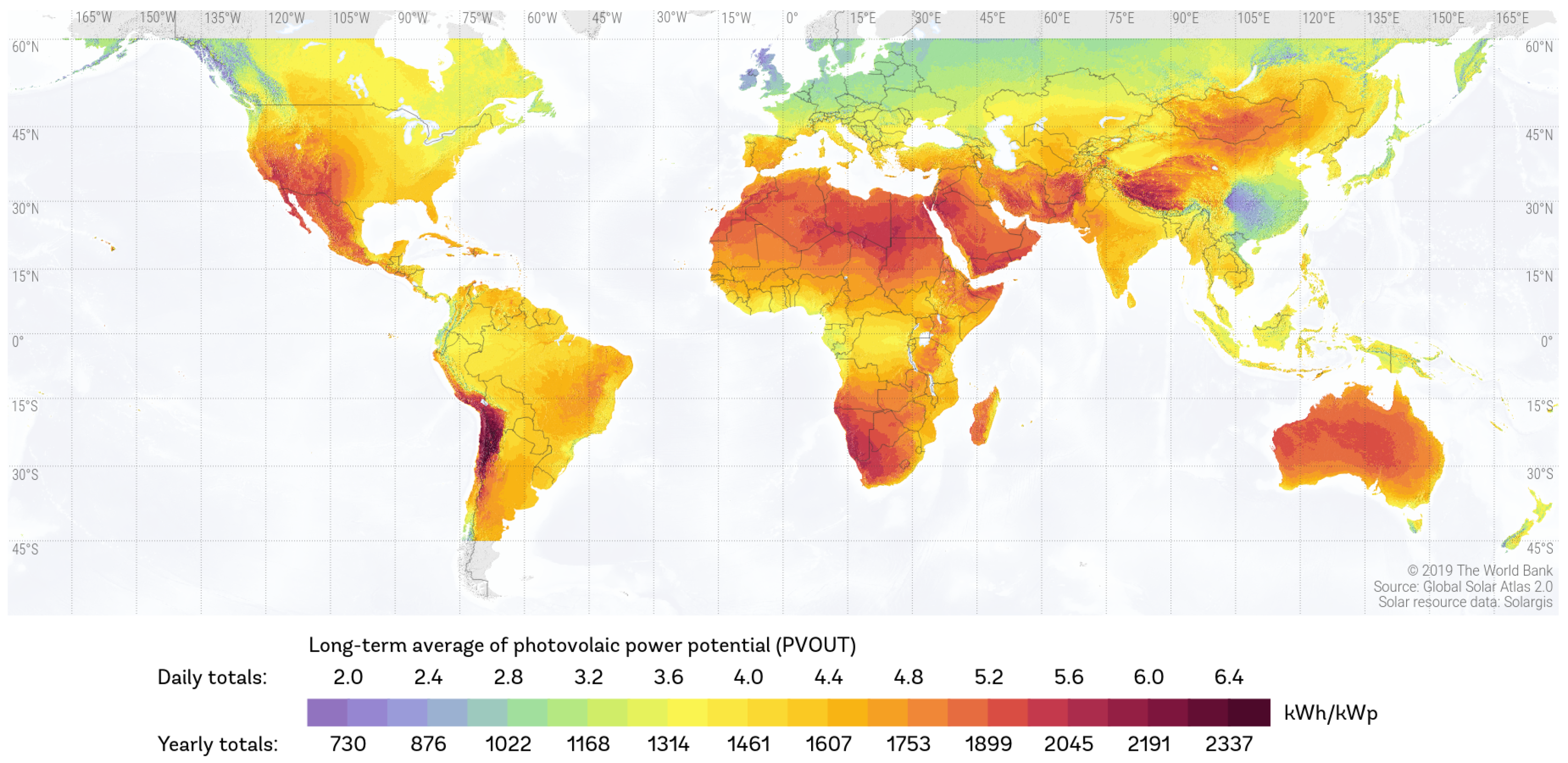
5]. In the context of growing energy development, the incorporation of renewable energy sources (RES) into contemporary power systems is increasingly reliant on hydrogen. Among the various RESs, solar energy stands out as the most widespread and promising resource for cleaner power generation. The Earth’s surface receives average solar radiation of approximately 1367 W/m
2, capable of generating a staggering 1.8 × 10
11 MW annually [
6]. This immense and pervasive energy supply is more than sufficient to effortlessly meet the world’s energy needs. The distribution of solar potential, as illustrated in
Figure 1, showcases enormous opportunities to harness solar energy on Earth.
The International Energy Agency (IEA) recognizes photovoltaics (PV) as one of the fastest-growing and most cost-effective renewable energy sources. Currently, PV forecasting research is considered a central focus among the major areas of prediction analytics. The production of PV power is highly influenced by meteorological variables, including solar radiation, clouds, humidity, pressure, temperature, etc. The inherently intermittent nature of these factors renders PV power production unpredictable, thereby impacting grid stability and the cost-effectiveness of power system operation [
7]. Therefore, the accurate prediction of PV power output is crucial to eliminate these uncertainties and fluctuations.
Forecasting PV power on an hourly to day-ahead basis offers numerous advantages, including optimized power dispatching, cost efficiency, and a dependable power supply. Accurate PV power prediction contributes to appropriate power dispatching, cost-effectiveness, and a reliable power supply. With precise forecasting, companies can avoid penalties, schedule supply offerings to the market as efficiently as possible, and enhance revenues [
8,
9]. Additionally, accurate forecasting can be used to make decisions regarding unit commitment, reserve needs, and maintenance planning to achieve the lowest possible operating costs. Considering these factors, accurate PV forecasting has been acknowledged as one of the major issues in power systems [
10].
Solar power forecasting can be categorized into physical, statistical, and machine-learning models. Numerous methods have been developed using both physical models and numerical approaches. Numerical weather prediction (NWP) is established based on structural and physical hypotheses [
11]. The chaotic nature of weather patterns and atmospheric uncertainties makes NWP computationally challenging and necessitates a greater operating cost. Additionally, these models must be developed for specific locations. The foundation of statistical models is the use of conventional regressive mathematical models like linear regression (LR) and autoregressive integrated moving average (ARIMA) models. Since LR models linearly map the target power and inputs, they are unable to effectively depict the nonlinear relationship between solar power’s input characteristics and outputs. Furthermore, the accuracy of these models declines as the forecasting horizon lengthens. To resolve these difficulties, several machine learning (ML) techniques have been developed.
Artificial neural networks (ANNs) and support vector machines (SVMS) are the most common ML models with strong nonlinear approximation capabilities [
12]. Since the 1980s, researchers have increasingly used ANNs. ANNs have gained popularity among researchers over statistical models due to a higher degree of accuracy and the nonlinearity of meteorological data. The most frequently used ANNs include the multilayer perceptron (MLP), feed-forward neural networks (FFNNs), radial basis neural networks (RBNNs), recurrent neural networks (RNNs), backpropagation neural networks (BPNNs), general regression neural network (GRNNs), and adaptive neuro-fuzzy interface systems (ANFISs) [
13]. A good comparison can be found in the work of Donnelly et al., which utilized Gaussian process (GP) models to emulate a hydraulic inundation model, enabling real-time flood depth predictions with uncertainty quantification [
14]. Their framework accurately reproduces water depths and the extent of inundation, surpassing a neural network-based emulator and offering significant computational speedups compared to the original simulator.
MLP is a type of supervised feed-forward ANN with one or more layers between its input and output layers. These layers, sometimes known as hidden layers, can be adjusted to fit the difficulty of a problem. FFNN is a less sophisticated ANN architecture in which information simply passes from the input layer to the output layer [
15]. On the other hand, an RBNN is considered a two-layer ANN, and the learning process can be divided into two distinct stages based on the weights of the synaptic connections [
16]. It performs well but requires time for the learning process. An RNN is effective at learning various computational structures and intricate interactions, making it a suitable tool for forecasting time-series data.
According to Yona et al., forecasting errors are significantly reduced with an RNN compared to an FFNN [
17]. BPNNs have garnered considerable attention among other ANN-related techniques due to their superior non-linear mapping function. An LSTM model, incorporating a clearness index method and k-means classification of the weather, has been introduced to enhance prediction accuracy on overcast days [
18]. Furthermore, a framework for partial daily pattern prediction (PDPP) has recently been proposed to improve time correction modification (TCM) in the LSTM-RNN model [
19]. However, the primary drawbacks of ANNs are overfitting and the substantial amount of data needed for training, increasing the complexity of implementation and costs in reality.
Support vector regressors are a type of machine learning model that can establish nonlinear relationships. Solar power forecasts have been conducted using support vector regression (SVR), considering various weather factors such as cloud cover and sun exposure [
20]. A hybrid technique combining genetic algorithms and an SVM has been developed to enhance accuracy compared to a simplified SVM [
21]. However, these models rely on the predetermined nonlinear mapping and parameters, making it challenging to fully comprehend the underlying nonlinear relationship between the inputs and the intended values [
22,
23].
In the present study, various research gaps were identified. These gaps encompass the need for a deeper understanding of the GPR model’s ability to capture underlying patterns when faced with noisy or outlier-laden data. Additionally, the manual tweaking of hyperparameters in the Bayesian optimizer, recognized as a time-intensive process, constitutes another area for exploration. It presents a methodical approach to applying Bayes’s theorem in order to update observed data with the prior understanding [
24,
25]. The study also suggests investigating the model’s adaptability to diverse time intervals and delving into the evaluation of objective functions in the presence of noise. To overcome these challenges, this study contributes to the following areas.
Enhanced Forecasting Accuracy: The proposed GPR model with Bayesian optimization demonstrates a significant enhancement (98% and 90%) in forecasting accuracy compared to alternative models like the feed-forward neural network and ANN. This highlights a substantial contribution to improving prediction outcomes.
Robustness and Flexibility: The integration of GPR with Bayesian optimization contributes to the model’s robustness and flexibility, especially in handling noisy and limited data. This adaptability ensures that the model remains relevant and useful in evolving environments.
Time and Resource Savings: Bayesian optimization is noted for its efficiency in systematically exploring the hyperparameter space, leading to potential time and resource savings. This contribution is particularly relevant in scenarios involving complex models and large data sets.
Handling Multivariate Analysis: The suitability of GPR for multivariate analysis is highlighted, showcasing its effectiveness in handling many input variables. This contribution is essential for addressing the complexities of associations between predictor variables and the target variable, such as in solar energy forecasting.
The subsequent sections of this paper are presented as follows: A literature review is provided in
Section 2; Data and data preparation are described in
Section 3 and
Section 4, respectively; An overview of the Bayesian optimizer is discussed in
Section 5. The proposed methodology is presented in
Section 6. Results and analysis with a comparison are discussed in
Section 7 and
Section 8 summarizes the conclusions and future work.
Figure 1.
World solar resources map [
26].
Figure 1.
World solar resources map [
26].
2. Literature Review
There are many forecasting algorithms presented in the literature on solar power forecasting. Dhillon et al. [
27] compared three models (feed-forward neural networks, backpropagation neural networks, and model-averaged neural networks) for forecasting solar energy in the field of precision agriculture to predict power for wireless sensor networks (WSNs). The model was developed using data from NREL’s (the National Renewable Laboratory’s) four-month period. Eight variables, including pressure, temperature, relative humidity, the dew point, wind speed, the hour of the day, the zenith angle, and historical solar intensity readings, were utilized to predict GHI for the next 24 h. The outcome showed that a feed-forward neural network provided the best result with the least memory needed (20 KBytes), and the values of the RMSE and the coefficient of correlation (
) were, respectively, 98.052 and 56.61. Elizabeth et al. [
2] proposed a unique multi-step CNN-stacked LSTM model with a dropout layer for the prediction of short-term solar irradiance and POA irradiance. The actual solar data were obtained from the Abu Dhabi-based Sweihan Photovoltaic Independent Power Project. The proposed model offered the best RMSE and
values of 0.36 and 0.98 for solar irradiance prediction and 61.24 with
0.96 for POA prediction, which also showed better performance compared to ML techniques such as LR, SVR, and ANNs with the same data set. To confirm the suggested architecture’s robustness, noise-injected data were also tested.
Khan et al. [
28] suggested that the most effective forecasting model for PV power output is recurrent neural networks. The data were provided from Quaid-e-Azam Solar Park in Bahawalpur, Pakistan, a 100 MW solar power plant. The study concluded that the bidirectional long short-term memory (LSTM) RNN framework outperformed the SARIMA model under all weather conditions (sunny, cloudy, rainy, partially cloudy, dusty, and foggy), particularly under cloudy weather conditions where the root mean square error (RMSE) was found to be the lowest at 0.0025,
was at 0.99, and the coefficient of variation of the root mean square error (CV-RMSE) was observed at 0.0095%. C.-H. Liu et al. [
13] proposed an ML methodology architecture based on LSTM and MLP with different train data set sizes from two PV sites, KHH (Kaohsiung) and MFU (Thailand), respectively. The result of the machine learning operations for data processing, model fitting, cross-validation, metrics evaluation, and hyperparameters tweaking demonstrated that the suggested simplified LSTM model performed better than the MLP model. The average RMSE was 0.512, which is highly encouraging and suggests that the proposed technique and architecture will work well for applications that require short-term solar power forecasting.
Vanderstar et al. [
29] proposed a method to anticipate two-hour-ahead solar irradiance levels using real-time solar irradiance measured both locally and at distant monitoring stations using an ANN at a site in Northwestern Alberta, Canada. The results of this study show that it is possible to use as few as five remote monitoring stations to achieve near-peak forecasting accuracy from the algorithm and that it is preferable to give the remote monitoring sites adequate geospatial separation around the target site, rather than clustering the sites in the strictly upwind directions. The RMSE was 10.8%, which is a comparatively low value.
Taoufik et al. [
30] proposed a solar energy predictor for communicating sensors or SEPCS. This prediction model makes short-term predictions about future energy availability based on historical energy observations. The authors used a database that identified the evolution of solar radiation over the course of a year to evaluate the performance of the suggested algorithm. Then, a performance comparison revealed that the SEPCS predictor greatly outperformed the most advanced energy predictors by lowering the average prediction error from 28 to 6.5%.
Zang et al. [
31] introduced two brand-new deep convolutional neural networks (CNNs), namely the Residual Network (ResNet) and the Dense Convolutional Network (DenseNet), as the main forecasting models. To build input feature maps for the two novel CNNs, a data preprocessing method involving historical PV power series, meteorological components, and numerical weather prediction was proposed. A meta-learning strategy based on a multi-loss-function network was introduced to train the two deep networks, ensuring high robustness of the extracted convolutional features with superb nonlinear representation abilities consisting of more than ten layers. The point forecasting mean absolute errors (MAEs) of the hybrid ResNet and DenseNet were 0.152 kW and 0.180 kW, respectively, according to a case study using a 5 kW capacity PV array. The coverage error rate of the two models in probabilistic forecasting was less than 5%, notably with the error rate of ResNet being less than 1%.
Perveen et al. [
32] used fuzzy logic and neural networks to construct their short-term PV power forecasting technique using a 15-year data set across India. Regression models and intelligent models were compared using statistical measures. The suggested model was used to forecast short-term PV power under a variety of climatic circumstances. The Adaptive Neuro-Fuzzy Inference System (ANFIS) model outperformed other models, according to simulation findings, for PV power forecasting. The greatest root mean square error (RMSE) for the suggested model was 0.5% on foggy days.
Ahmed et al. [
33] conducted a statistical comparison among seven brain models to ascertain the global solar radiation (GSR) in Qena, Egypt. In contrast to other models, the study showed that the artificial neural network (ANN) model produced good outcomes. Comparing models and assessing the importance of the anticipated data are both possible using the test of the mean values of the mean bias error (MBE), RMSE, mean percentage error (MPE), Nash and Sutcliffe efficiency (NSE), and
. The hydraulic system’s calibration criteria included the NSE metric, which provides a better comparative outcome.
Asl et al. [
34] introduced solar energy prediction in Dezful, Iran (positioned at 32.1648° N and 48.25° E) using a linear transferable Levenberg–Marquardt (LM) method based on a multi-layer perceptron neural network (MPL NN) and taking the input parameters as the relative humidity, the daily mean air temperature, evaporation, the soil temperature, the day of the year, daylight hours, and the wind speed. The MPL has three neurons in the first hidden layer and two in the second hidden layer with the sigmoid transferred function, which produces the best prediction outcomes. The findings of the testing data showed that the mean absolute percentage error (MAPE) equaled 6.08%, while
equaled 99.03%, and the training data showed that the mean square error (MSE) equaled 0.0042 and the standard error of estimate (SEE) equaled 5.9278, which is suitable for estimating global solar radiation (GSR).
DURRANI et al. [
35] proposed an irradiance forecasting system based on multiple feed-forward neural networks for predicting the PV yield. Five years’ worth of historical meteorological data were used to train the proposed irradiance forecast model’s neural networks. For Stuttgart, the mean absolute percentage inaccuracy of the global horizontal irradiance forecast was 3.4% on sunny days and 23% on gloomy days. Sunlight, cloudiness, and temperature have a greater impact on the Global Horizontal Irradiance (GHI) neural network forecast model than other inputs. The research concluded that this system’s PV power forecast surpassed that of the PV persistence power forecast model.
Al-Shamisi et al. [
36] used the artificial neural network (ANN), multi-layer perceptron (MPL), and radial basis function (RBF) methodologies with the input parameters of sunshine hours, the maximum temperature, the mean relative humidity, and the mean wind speed to perform a research study in the UAE’s Al-Ain city (located at 24.1302° N and 55.8023° E). A 3-year sample of data (2005–2007) was used for testing, while the statistical values for the 10-year period (1995–2004) used to train the network were
, the root mean square error (RMSE), and the mean bias error (MBE). The findings of 11 models with varied input layer parameters demonstrated that, in the majority of circumstances, the RBF technique was superior to the MPL technique.
Wang et al. [
37] introduced a brand-new hybrid model with adaptive learning for forecasting solar intensity. It is an online forecasting technique, and as data volumes rise over time, the system’s effectiveness gets better. The UMASS Trace Repository data set, which captures solar intensity in watts/m
2, and meteorological data regarding four weather parameters (temperature, humidity, the dew point, wind speed, and precipitation), was used to test the suggested technique. The authors claimed that, after six months, the average monthly RMSE fell from 28.38 to 14.72 W/m
2.
Jensona et al. [
38] worked with two data sets: solar radiation data (SoDa) and the National Center for Environmental Predictions (NCEP) to predict the average daily solar irradiance using two models (a radial basis function network (RBFN) and a backpropagation neural network (BPN)). Data from two years were used to train the network, while data from one year were utilized to test it. For the two data sets, 3.12 MJ/m
2 and 3.212 MJ/m
2, respectively, the RMSE values were shown to be lower for BPN.
Manjili et al. [
39] established an adaptive system for day-ahead solar intensity forecasting using data from NREL. The proposed approach was distinctive in that it combined statistical and artificial intelligence techniques. Time, temperature, relative humidity, zenith angle, azimuth angle, total cloud cover, opaque cloud cover, and pressure were the eight weather characteristics that were fed into the model. The method’s root mean square error (RMSE) was determined to be 149.29 W/m
2.
Zhang et al. [
40] presented different deep convolutional neural networks (CNNs) using high-resolution weather forecast data, investigating various temporal and geographical connectivities to capture the cloud movement pattern and its impact on forecasting solar energy generation for solar farms. It was able to lower the error rate from the persistent model’s 21% to 15.1% from the support vector regression (SVR) models and 11.8% from the convolutional neural networks compared to the state-of-the-art forecast error rate. Due to the use of high-resolution weather data in the training data set, the research found that deep learning models performed better in predicting solar energy generation than the earlier physical models.
Haixiang et al. [
41] proposed the hybrid method of variational mode decomposition (VMD) and a deep convolutional neural network (CNN) with multiple input factors, which was capable of enhancing the accuracy of short-term PV power forecasting. Compared to other 1D VMD-based forecasting approaches, the model’s prediction accuracy was higher because it was trained on correlations in both hours and days. When developing new CNN models, transfer learning is crucial. The study came to the conclusion that deep learning models beat conventional physical models when it comes to predicting solar energy outputs.
Lee et al. [
42] proposed a novel deep neural network that can be trained to estimate the amount of solar energy that would be produced the next day using time series data gathered from photovoltaic inverters and national weather centers. The study refers to integrating two CNNs with filters of various sizes in order to effectively identify local short-term characteristics and efficiently capture long-term features. With roughly estimated weather data, the suggested method accurately predicts solar power and operates reliably without sophisticated preprocessing to weed out outliers. The network surpasses a number of conventional regressors as well as a cutting-edge deep neural network-based solar power prediction algorithm.
Table 1 summarizes insights from various works in the literature on key research aspects. It provided a vital foundation for our planned investigation by pointing out patterns and gaps in the literature. Recognizing fundamental limitations, it became our starting point for our research, shaping our contributions. Through this synthesis, we aimed to build upon existing knowledge and address identified gaps in the current state of research.
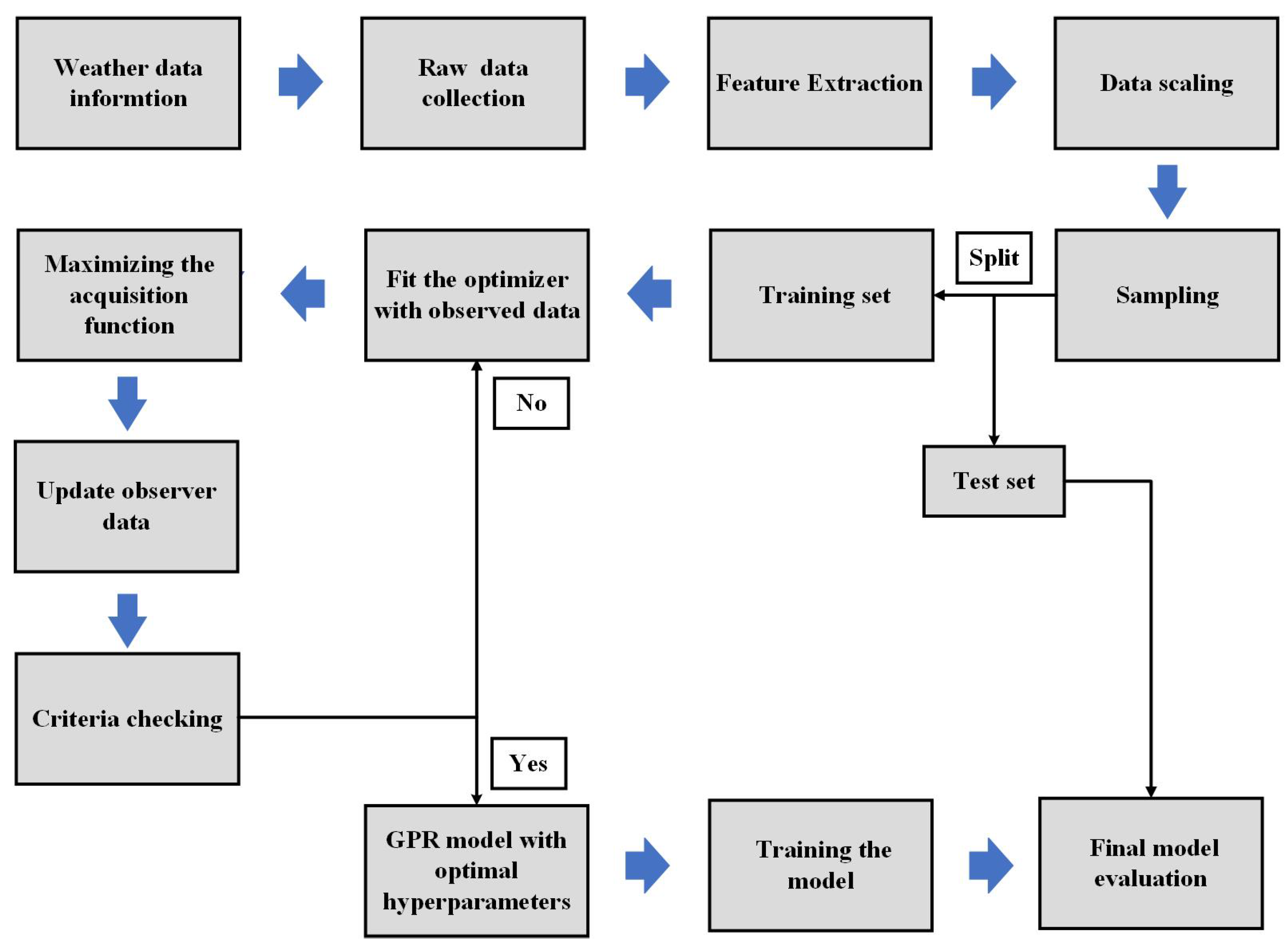
5. An Overview of Bayesian Optimizer
Hyperparameters play a crucial role in ML algorithms since they directly dictate the behavior of training algorithms and significantly impact the performance of the resulting models. Various techniques have been developed and successfully applied in specific domains, although their implementation often requires specialized knowledge and expert experience. In some cases, brute-force search methods are employed due to the complexity of the problem. Consequently, the development of an efficient hyperparameter optimization algorithm capable of optimizing any given machine learning method would greatly enhance the overall efficiency of the learning process. This research aims to establish a relationship between the performance of ML models and their respective hyperparameters through the utilization of Gaussian processes. By doing so, the problem of hyperparameter tuning can be abstracted as an optimization problem, and Bayesian optimization is employed to address it. Bayesian optimization operates on the principles of the Bayesian theorem, in which a prior distribution is established over the optimization function, and information from previous samples is used to update the posterior distribution of the function [
43]. A utility function is then employed to select the next sample point that maximizes the optimization function. It consists of three fundamental components: a search space that encompasses potential parameter samples, an objective function, and a surrogate. It constructs a probabilistic model of the objective function, utilizing this model to identify the most auspicious hyperparameters for assessment against the genuine objective function.
The above equation reflects the core concept of Bayesian optimization. Here,
A′ represents
x’s search space. The fundamental purpose of Bayesian optimization is to integrate the a priori distribution of the function
f(
x) with the empirical evidence in order to derive the posterior distribution of said function. Subsequently, this posterior information is utilized to identify the optimal location of the function
f(
x) based on a specified criterion. This criterion is enacted via a utility function, u, which is also known as the acquisition function.
The core idea of Bayesian optimization is deduced from Bayes’s theorem. For instance, if
V is the presented evidence data, the probability of posterior function
P(M|V) for model
M is equal to the product of the prior probability
P(M) and
P(V|M). Here,
P(V|M) explains how well the model explains the observed data, in which
(V) is the observing data for a given particular model,
M.For can be found optimizing the acquisition function u using function f. denotes the training data set consisting of samplings of function f. Then, observe the objective function . This process is repeated until either the maximum number of iterations is reached or the difference between the current value and the ideal value acquired thus far is less than a predetermined threshold. It can be noted that, compared to other optimization techniques, Bayesian optimization does not require the explicit definition of function f.
7. Result and Analysis
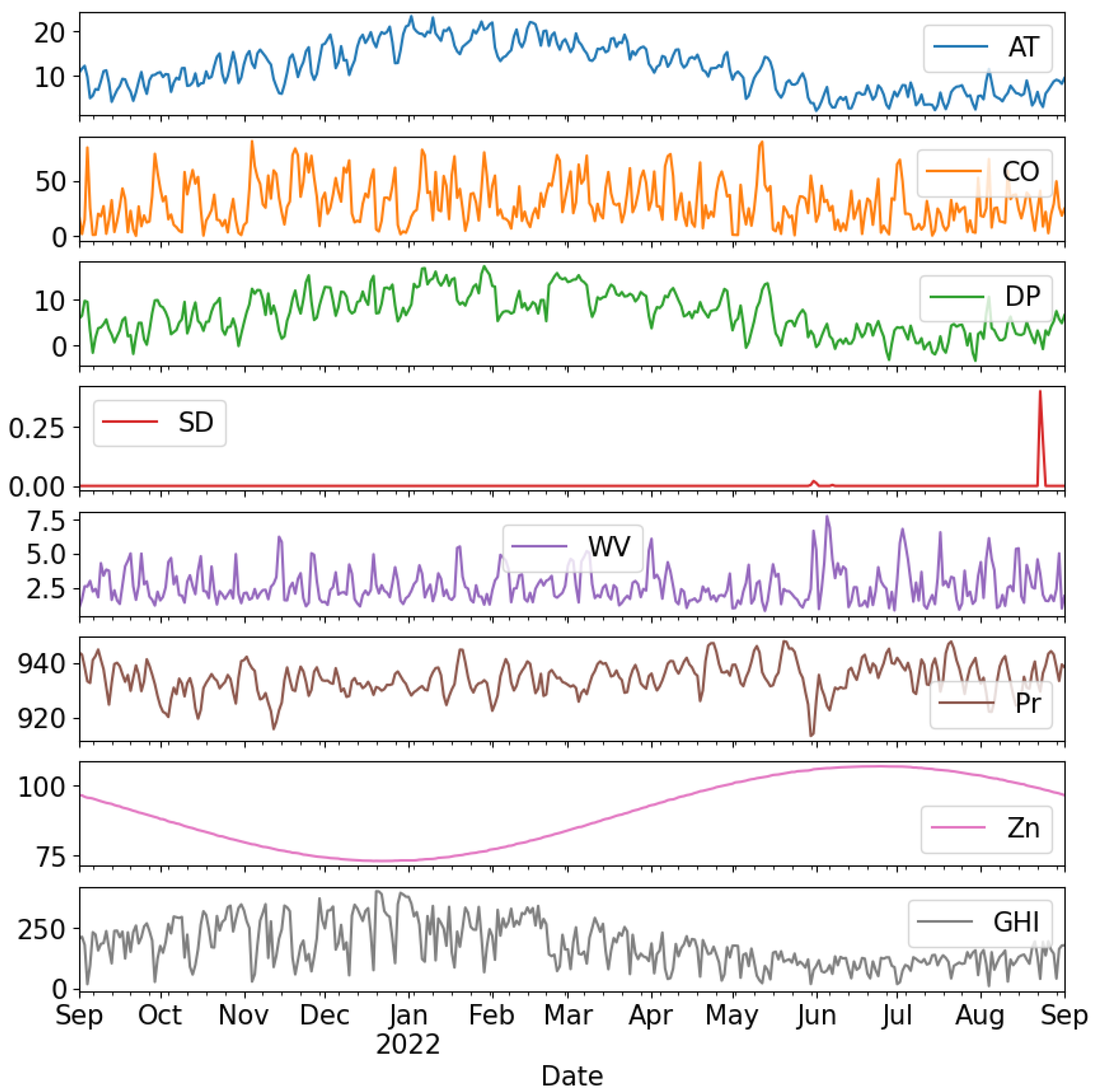
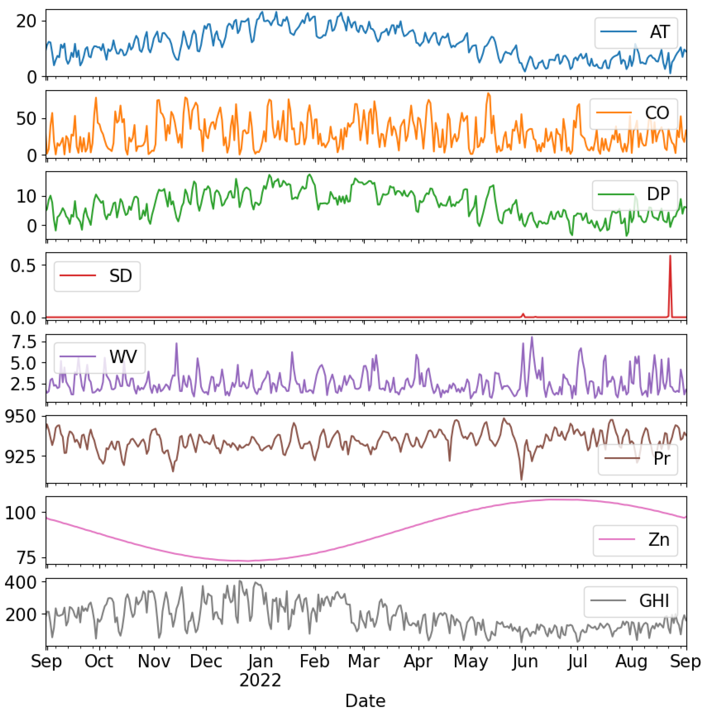
The primary objectives of this work were to analyze the performance of various ML-based forecasting techniques, such as LSTM, GPR, and a proposed GPR with a Bayesian optimizer, to predict the GHI. Moreover, some conventional machine learning models were also evaluated and compared with the proposed techniques. To assess the feasibility of this study, two different solar data sets with different sampling times from Canberra, Australia, provided by Solcast, were used. Forecasting performance was measured using various performance evaluation metrics. The data were divided into a percentages of 70–30 for the training set and the testing set. Simulations and programming were conducted in a Python environment using Google Colabratory.
7.1. Performance Evaluation Matrices
As discussed above, the following performance measuring metrics were used in this study to assess the performance of the forecasted model: the root mean square error (RMSE), mean square error (MSE), the determination of correlation coefficient (), and the mean absolute error (MAE). These metrics were considered to evaluate the model’s performance. Lower values of these metrics indicate better predictive results. In the following discussion, n represents the total number of samples, represents the actual values of forecasting variables, and represents the predicted solar power.
(a) Root mean square error (RMSE): The RMSE is the square root of the average of the squared differences between actual vs. predicted values:
(b) Coefficient of determination (
):
denotes the percentage of variance in actual values that can be explained using expected values. It has a scale from 0 to 1, with 1 indicating a perfect fit:
where
is the mean of actual solar power.
(c) Mean square error (MSE): It is the average of the squared differences between the predicted and actual values:
(d) Mean absolute error (MAE): The absolute value of the difference between the actual value and predicted values:
(e) Average absolute error (AAE): AAE calculates the average absolute difference between each predicted and actual value:
(f) Average biased error (ABE): ABE calculates the average difference between each predicted and actual value:
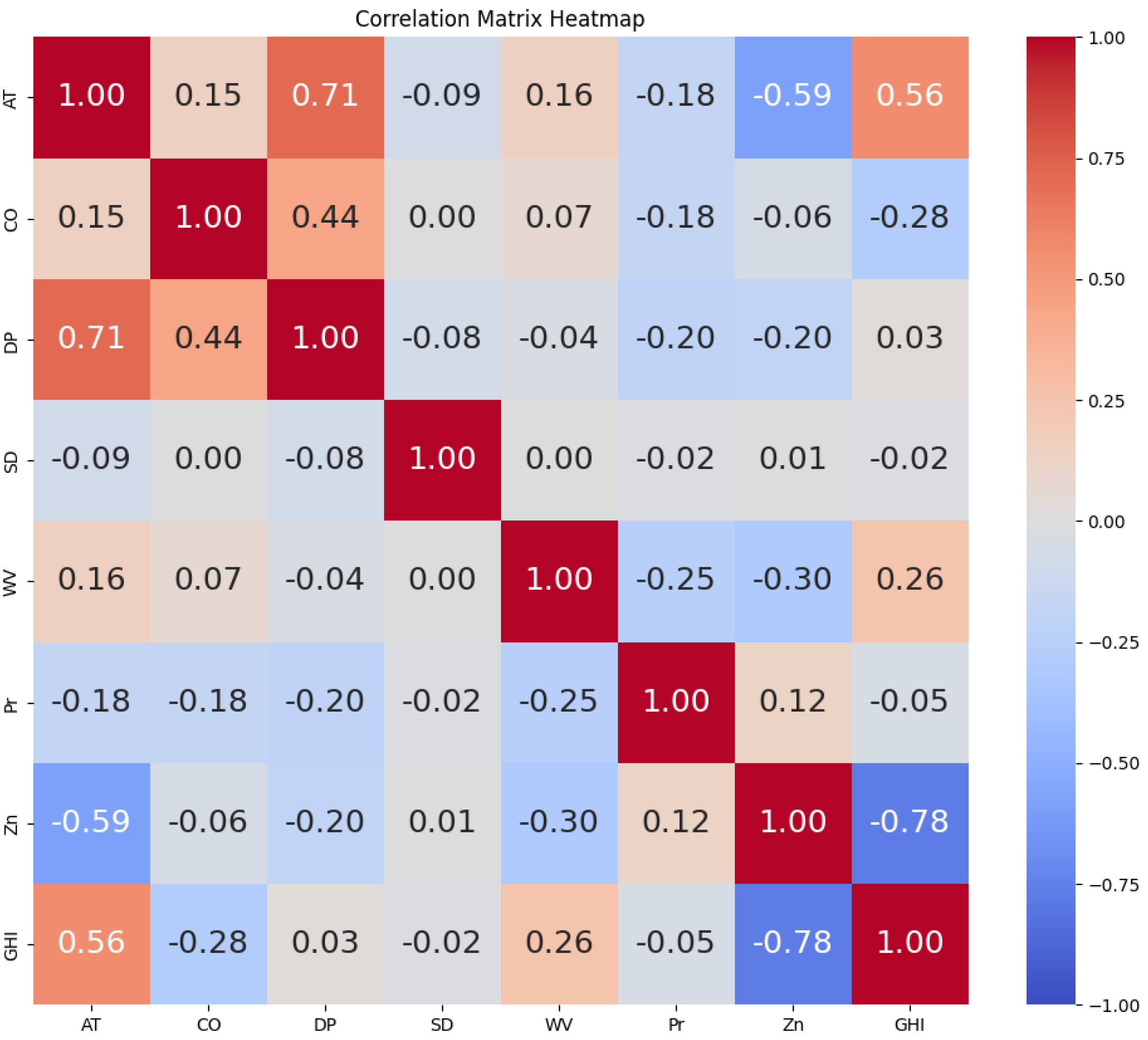
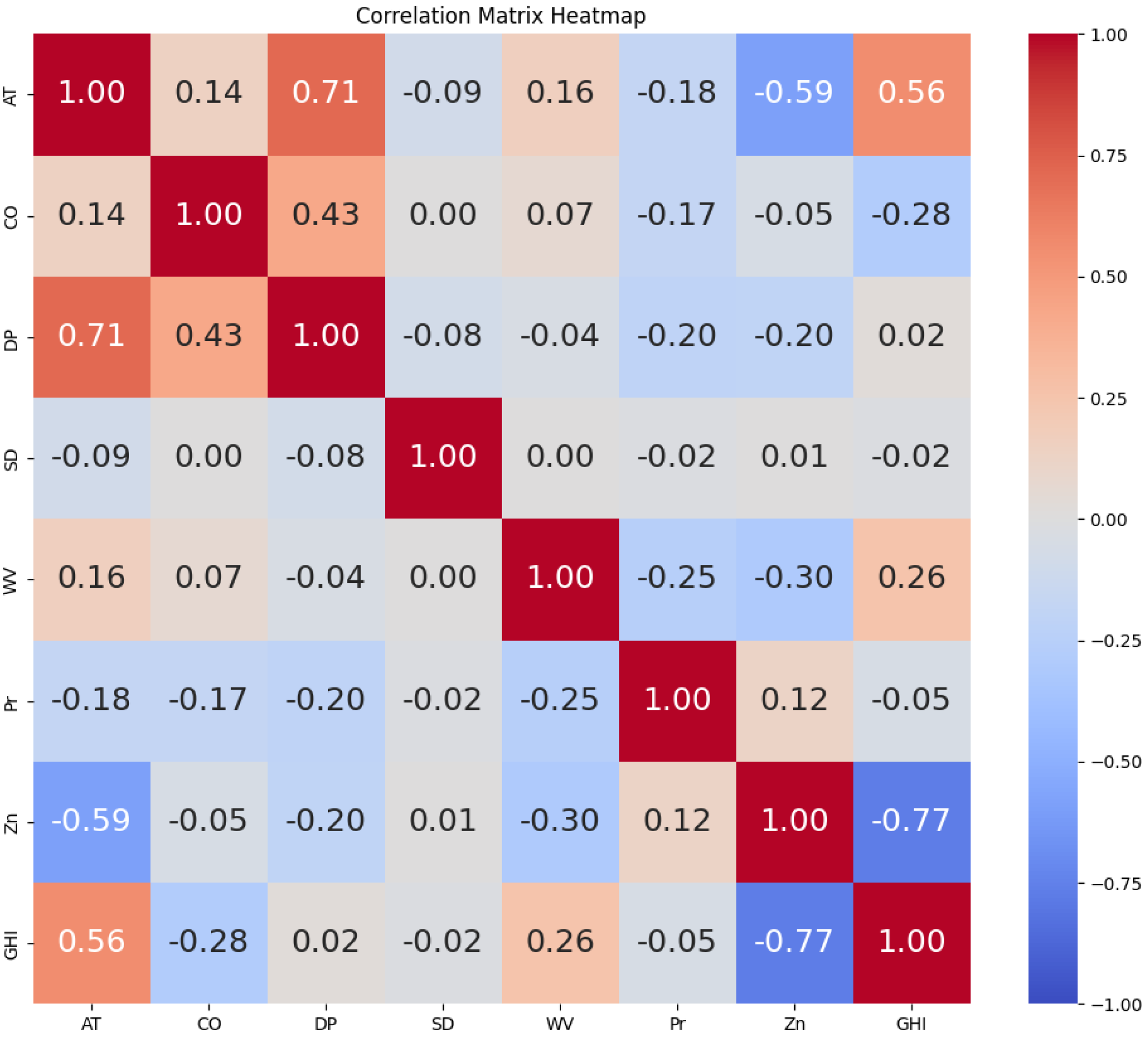
In this section, the collected solar irradiance data are used to test the performance of the proposed methodology. This study employed a multivariate analysis approach, utilizing two distinct data sets that exhibited varying time intervals between each sample. One of the experimental conditions involved a 60-min gap between each sample, whereas the other condition involved a 30-min interval. Under both conditions, we used four columns as input variables to estimate GHI. The comparison between the observed solar irradiance values and the anticipated values is illustrated in figures for seven different models: RF, MLP, SVR, regression, LSTM, GPR, and the suggested GPR with a Bayesian optimizer. It provides insight into the performance of all the methods discussed so far. The test performance accuracy and flexibility are discussed in
Table 2 using six error matrices (RMSE, MSE, MAE,
, AAE, and ABE), as described previously [
44,
45]. The value of the
closeness to 1 indicates a more accurate model. The RF, MLP, SVR, and regression models all performed well in terms of computing time, finishing their calculations in less than 60 s. On the other hand, the GPR model required a significantly longer processing time—roughly 368 s on average. In a comparable manner, the suggested model and LSTM model showed higher computing demands, averaging 406 and 476 s, respectively. The aforementioned results highlight the greater computational load linked to GPR, LSTM, and the proposed model in contrast to RF, MLP, SVR, and conventional regression techniques. From
Table 2, it can be seen that the GPR model, LSTM model, and GPR with a Bayesian optimizer outperformed all the other models. The GPR model for the 60-min interval performed the prediction task with the following error metrics: RMSE = 1.80, MSE = 3.24, MAE = 1.06,
= 0.97, AAE = 0.279%, and ABE = 0.018%. And for the 30-min interval, the obtained error metrics were as follows: RMSE = 1.89, MSE = 3.57, MAE = 1.13,
= 0.96, AAE = 0.576%, and ABE = −0.549%. However, the LSTM architecture performed better than GPR for both time intervals with the following error metrics: RMSE = 1.28, MSE = 1.64, MAE = 0.94,
= 0.99, AAE = 0.706%, and ABE = −0.509% for the 60-min interval and RMSE = 1.17, MSE = 1.37, MAE = 1.15,
= 0.99, AAE = 0.619%, and ABE = −0.615% for the 30-min interval. Lastly, it can be observed that the proposed GPR with a Bayesian optimizer model outperformed other previously stated deep learning and ML models for all performance matrices. The performance results are noted as RMSE = 1.09, MSE = 1.18, MAE = 0.49, and
= 0.99 for the 60-min interval, and for the 30-min interval, the obtained performance metrics were RMSE = 1.12, MSE = 1.25, MAE = 1.25, and
= 0.99. The advantages of GPR, LSTM, and the suggested model exceeded the disadvantages even though their computing times were longer. On the other hand, even if certain models have quicker computation times, their poor efficiency makes them inappropriate for practical usage. This emphasizes the trade-off between predicted accuracy and computing efficiency, with the latter being more crucial when choosing a model.
It can be shown that, of the seven models utilized under both the 30-min interval and the 60-min interval circumstances, GPR with a Bayesian optimizer achieved the best performance measure scores. The performance metrics of each tested model are presented in
Table 2, and the used model parameters and optimal values are shown in
Table 3. The best-performing hyperparameters for LSTM and GPR were chosen through manual testing. On the other hand, a Bayesian optimizer was employed to find the optimal parameters for our proposed model. A predefined range was provided to the Bayesian optimizer to explore it in order to identify the optimal hyperparameters. The optimizer successfully suggested the optimal hyperparameters to optimize model performance. This approach improved the predictive accuracy and automated hyperparameter selection.
7.2. Comparative Analysis
Here, a comprehensive analysis is carried out on each model that underwent testing. Furthermore, the outcomes derived from our data sets are shown. Each graph in this section consists of the first 100 samples that were obtained from our test data.
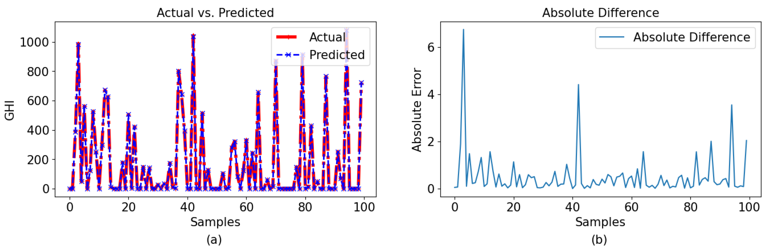
The figures indicate that the GPR model achieved comparable performance for both data sets depicted in
Figure 9a for a 60-min interval and
Figure 10a for a 30-min period. Despite being the least efficient among the three models, GPR exhibited acceptable performance in terms of usability. Due to the minimal difference between the actual and anticipated data, identifying any distinctions in the plots became challenging. The difference between the observed and forecasted values is shown in
Figure 9b and
Figure 10b, representing the 60-min and 30-min intervals, respectively. While the majority of the observed data points exhibited differences of less than 2 for 60-min intervals and 1.5 for 30-min intervals, it is worth noting that a significant number of samples displayed larger disparities. Some of them almost achieved as high a difference as 5 (30 min) and 3 (60 min).
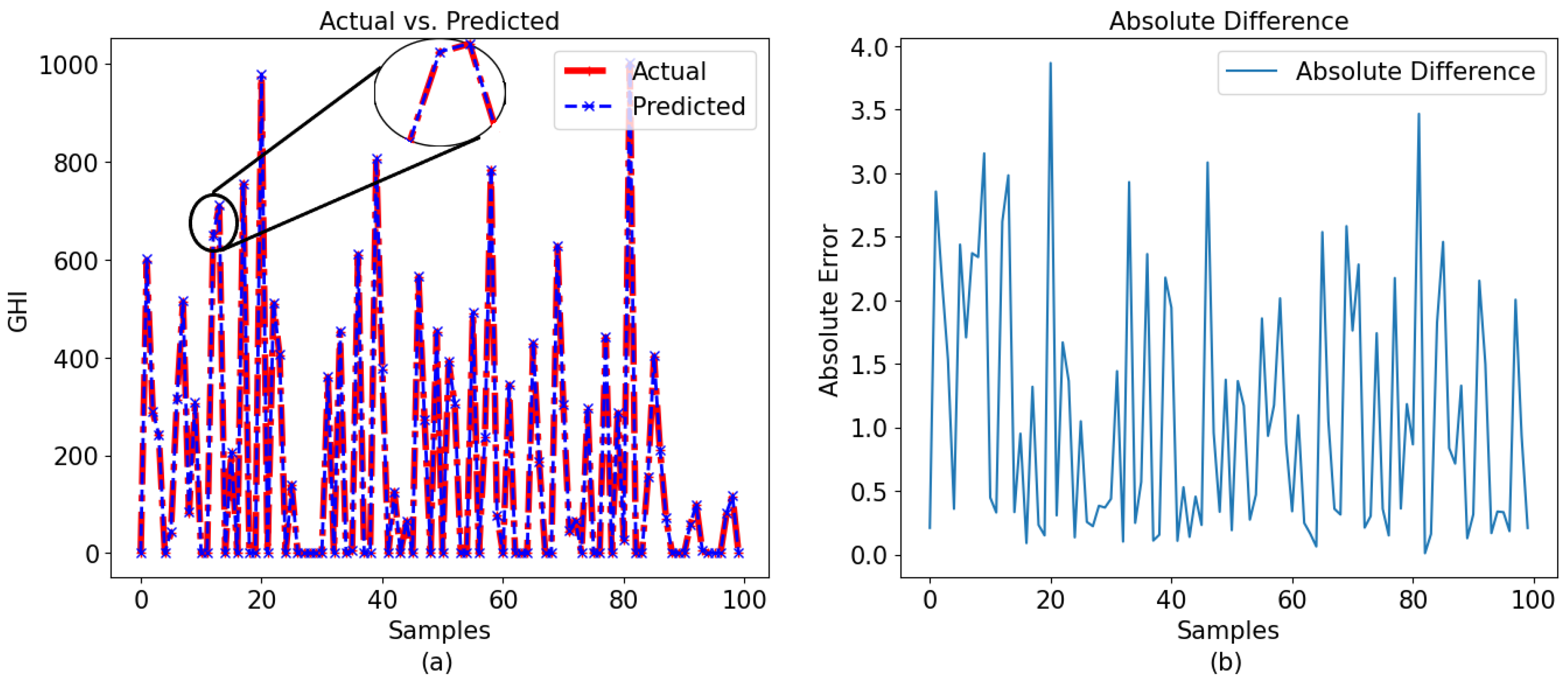
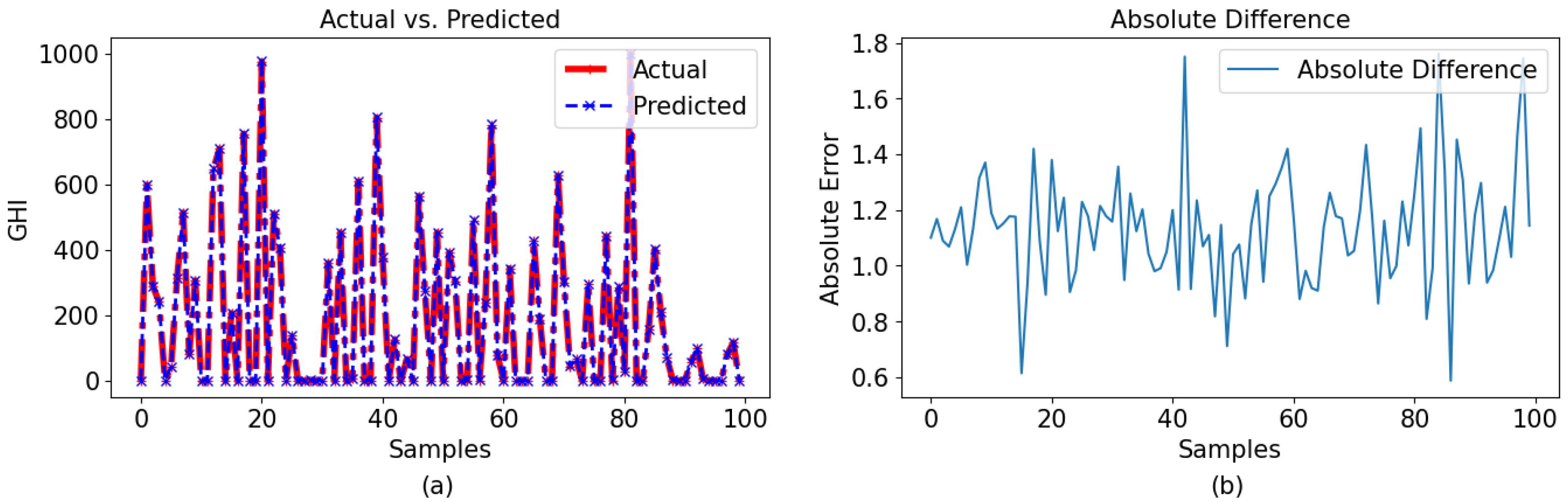
The similarity between the LSTM model and the GPR model was also noted. The LSTM model exhibited superior performance compared to the GPR model, with an
score of 0.99 in both instances. This demonstrates that the model performed flawlessly. The data seen and anticipated for various time intervals are depicted in
Figure 11a and
Figure 12a. In a similar manner, the distinctions between the observed and anticipated values are graphically shown for each sample in
Figure 11b and
Figure 12b.
In
Figure 11b, it is observed that, even though the LSTM model kept the difference low for the 60-min-interval data set, it failed to maintain the same performance for the 30-min-interval data set.
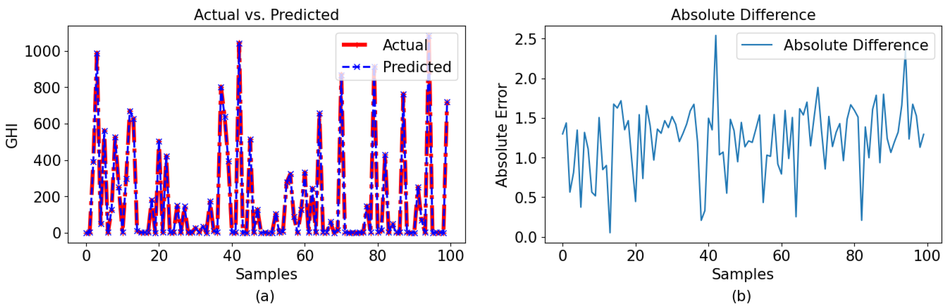
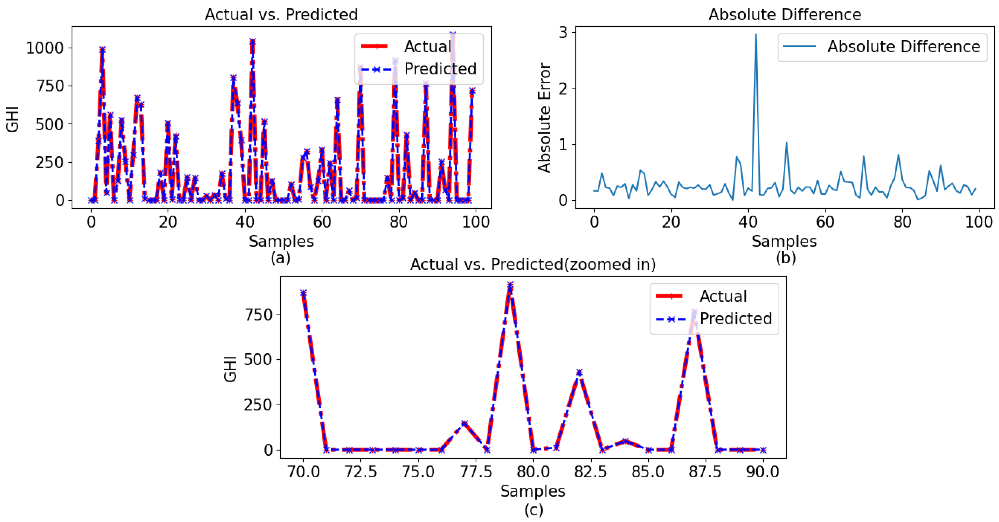
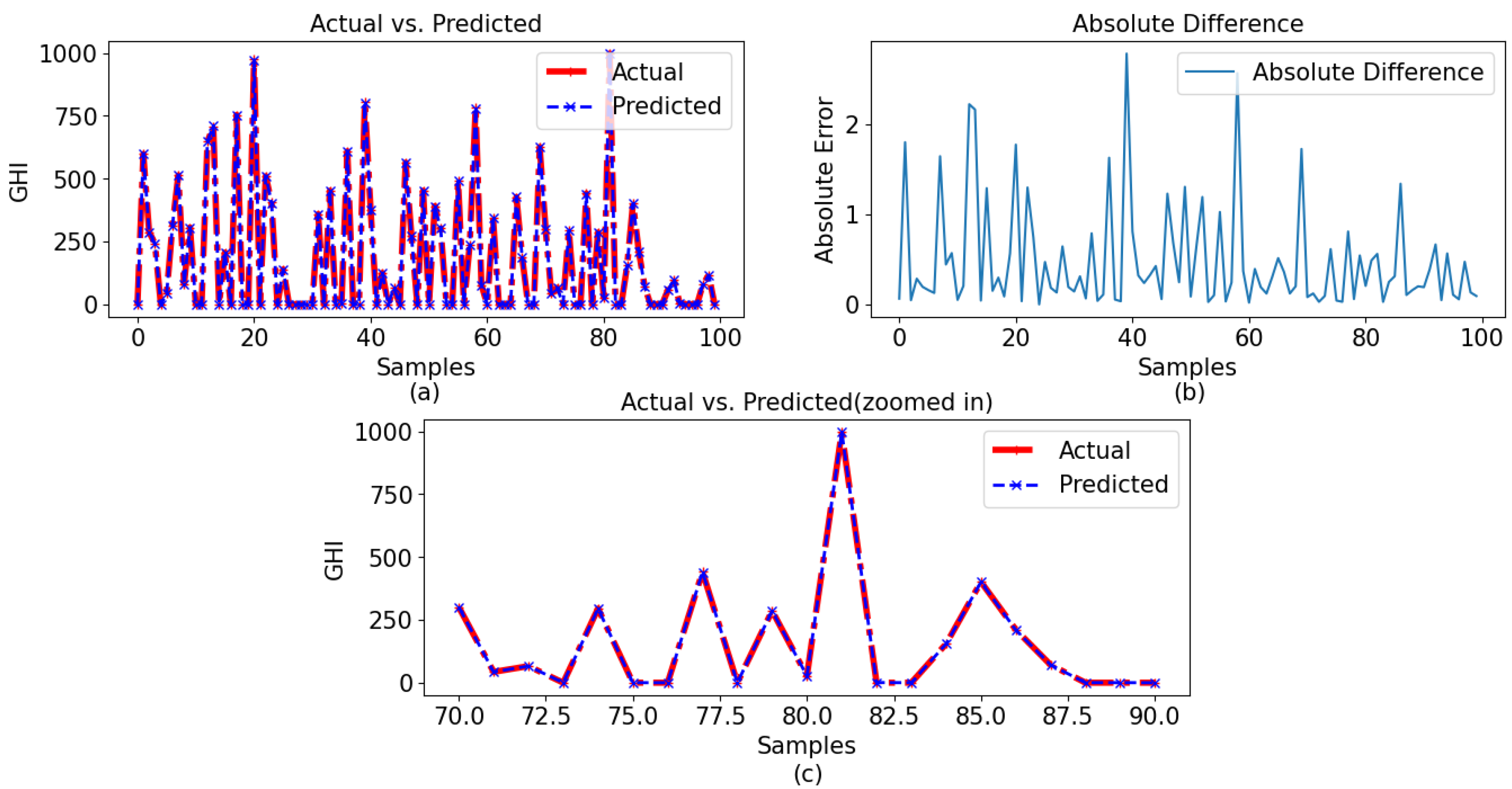
The GPR model with a Bayesian optimizer demonstrated superior performance compared to the other two models, which is clearly indicated in the graphical representations. The comparison between the observed and predicted results for the 60-min and 30-min intervals using GPR with a Bayesian optimizer is illustrated in
Figure 13a and
Figure 14a, respectively. Given the model’s impressive performance metrics, the figures presented in
Figure 13b and
Figure 14b illustrate the differences between the actual and predicted values for data sets with 60-min and 30-min intervals, respectively. In these figures, it can be observed that the model predicted very close values to the observed data. Here, it is also noticeable that the model worked better for the 60-min-interval data set compared to the 30-min interval data set.
Figure 13c and
Figure 14c present the zoomed-in version of the observed and predicted values for data sets with 60-min and 30-min intervals, respectively.
Here, the proposed methodology is compared with other models from the literature review, as detailed in
Table 3.
7.3. Discussions
The comparative advantage of GPR with Bayesian optimization over alternative neural network models, such as long short-term memory (LSTM) and other used models in the context of this forecasting task, can be related to a number of crucial variables. Bayesian optimization is a highly effective method for optimizing hyperparameters, particularly in the context of GPR models. This approach addresses the natural challenge of tuning hyperparameters in neural networks that possess a large number of such parameters. Additionally, the built-in characteristics of GPR, such as its ability to resist overfitting and provide uncertainty estimates, contribute to its robustness as a suitable option for forecasting applications. Moreover, the capability of GPR to effectively handle multivariate data, along with the systematic method of Bayesian optimization, significantly contributes to its effectiveness in this particular situation. The selection between GPR and neural networks is dependent upon the unique attributes of the job, the quantity of the data set, and the modeling prerequisites. In this regard, GPR presents itself as a persuasive alternative for accurate prediction, and in our case, it outperformed neural network models like LSTM.
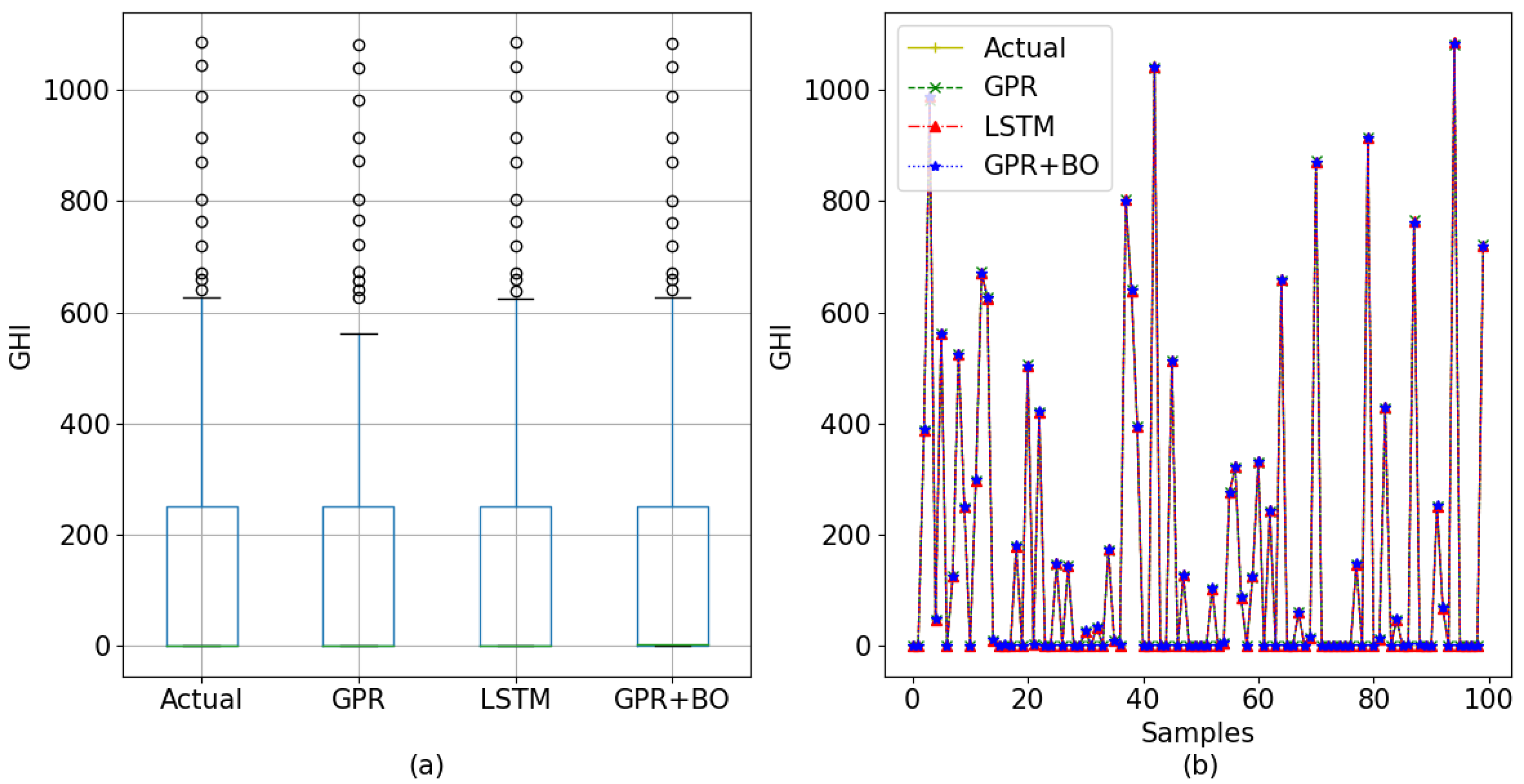
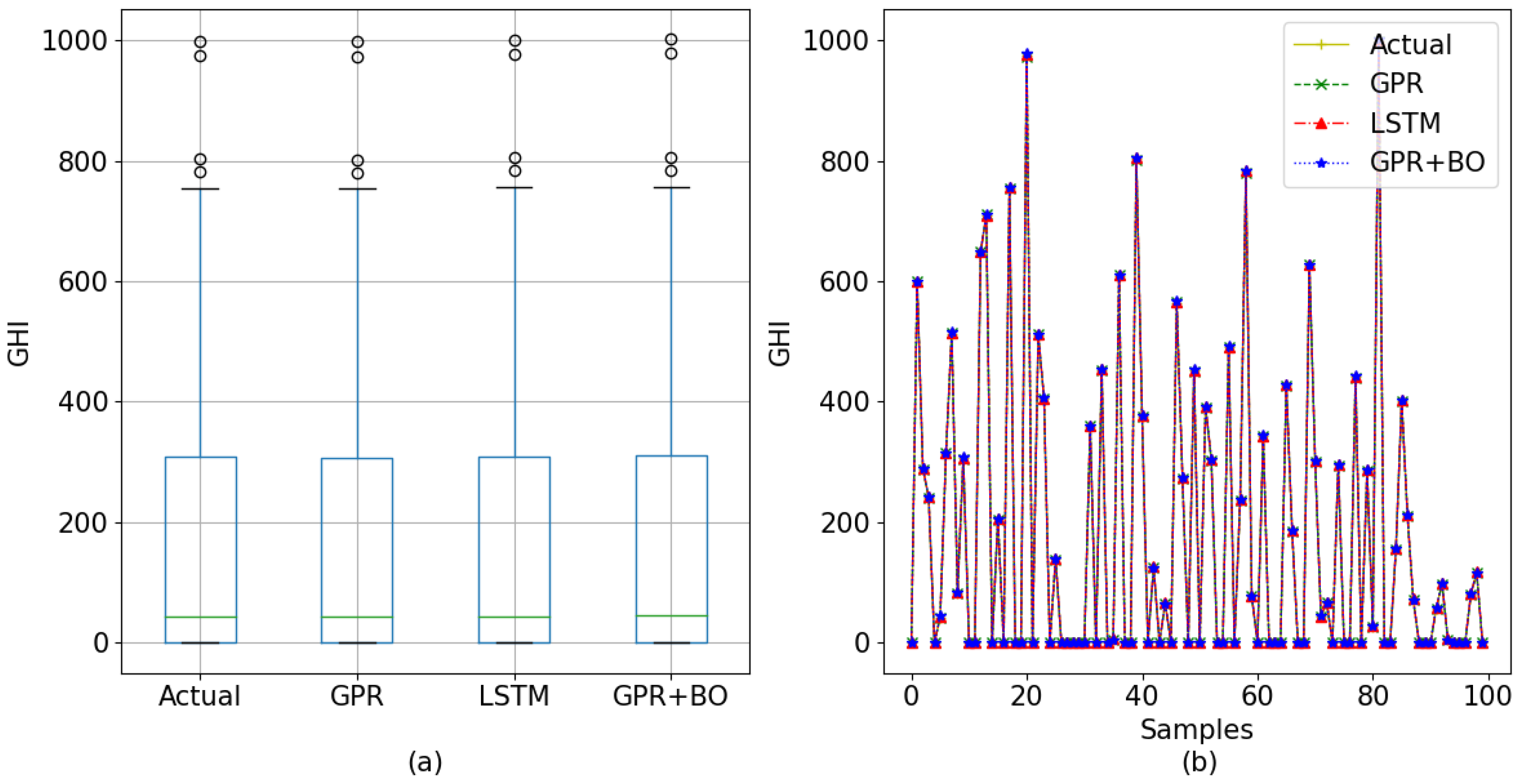
In
Figure 15 and
Figure 16, all three models’ prediction and the actual data are displayed utilizing line charts for 60-min interval data and 30-min interval data, respectively. To understand the actual value and predicted value of the models, a box plot of 60-min-interval data and 30-min-interval data is also included in the figures. Here, for the box plot, all the test data and their corresponding predicted data were used.
7.3.1. Gaussian Process Regression (GPR)
The GPR model is a model based on probability that presumes a Gaussian process to describe the connection between input and output data. The present work employed GPR with the utilization of the RBF kernel, which includes hyperparameters such as the length scale and alpha. The initial configuration for GPR entailed the selection of the RBF kernel with certain hyperparameters, namely a length scale of 1 and an alpha value of 0.01. The number of optimizer restarts (five) was selected to ensure that the model underwent optimization iterations in order to refine the hyperparameters.
The strength resides in its capacity to effectively represent complex linkages and uncertainties. The selection of the kernel and hyperparameters has a significant impact on the model’s ability to accurately fit the given data and effectively generalize to unseen samples. However, when considering the used data sets, it was observed that the link between the inputs and outputs was intricate, resulting in difficulties for the GPR model in accurately capturing it.
Another crucial aspect to consider is the process of hyperparameter tweaking. The performance of the GPR model is heavily influenced by its hyperparameters. When the Bayesian optimization process is not employed to tune the GPR model, it may not be optimized with the most suitable hyperparameters. Consequently, this can result in inferior performance metrics compared to the other three models that were tested. The GPR model requires effective feature engineering; yet, in our particular scenario, the data exhibited complexity, and the inputs shown limited the correlation with the output. Despite the model’s somewhat lower performance among the three, it nonetheless exhibited favorable performance metrics, indicating its usability.
7.3.2. Long Short-Term Memory (LSTM) Networks
LSTM is a recurrent neural network (RNN) that is well suited to managing sequential data. As our data set contained time-series data, LSTM effectively incorporated these dependencies, which may not have been possible for the other models. LSTM is a deep learning model that can automatically acquire hierarchical, complex features from data. It can model complex relationships between input characteristics and the objective variable. As a probabilistic model, GPR may not be able to capture such complex patterns. LSTM can simultaneously learn feature representations and temporal dependencies, which is advantageous when the input–output relationships are not expressly known and must be learned from the data. In addition, LSTM allows for parameter tuning during training, which improves model performance. LSTM can acquire relevant features automatically from the data, reducing the need for manual feature engineering. In coping with our complex data sets, this was a significant benefit. Because of these benefits, LSTM outperformed GPR and demonstrated superior performance metrics. The result is notable when observed in the plots shown in the previous section.
7.3.3. GPR with Bayesian Optimizer
GPR with a Bayesian optimizer performed the best among the three models used for analysis, while GPR performed marginally worse than LSTM and the proposed model. The Bayesian optimizer is the deciding factor in this case. The results can be seen in the case of both data sets in the observed and predicted data given below for the 60-min interval and the 30-min interval, respectively, in
Figure 15 and
Figure 16.
Bayesian optimization represents a sophisticated and effective approach to systematically investigating the hyperparameter space of ML models. In contrast to computationally expensive methods such as brute force, grid search, or random search, Bayesian optimization employs a proactive strategy by constantly selecting hyperparameter combinations that are more likely to produce improved outcomes. The previously discussed efficiency has the potential to result in substantial time and resource savings, particularly in situations involving complex models and large data sets. It also allows the model to adapt to the specific characteristics of the data. The method begins by establishing an initial collection of hyperparameters and afterwards iteratively improving them to correspond with the observed performance of the model. The capacity to adapt is of the highest priority when working with data sets that exhibit diverse time intervals, as it enables the model to flexibly change its behavior in order to accurately capture the underlying patterns. Bayesian optimization automates the process of hyperparameter tuning. It intelligently chooses the next set of hyperparameters to evaluate based on past observations, guided by an acquisition function. This automation simplifies the model development process and reduces the need for manual trial-and-error tuning.
GPR is a highly suitable method for conducting multivariate analysis due to its ability to successfully handle many input variables. In the present study, the input factors were demonstrative of a complex association between the predictor variables and the target variable, which is the GHI. GPR is particularly suited to collecting data on complex and non-linear interactions like these. The model is probabilistic in nature, so it includes both predictable predictions and the ability to measure the level of uncertainty associated with these predictions. The ability to evaluate the certainty of a model’s predictions is of significant importance in the context of forecasting work. The utilization of Bayesian optimization, when combined with GPR, enables the optimization of hyperparameters by taking into account both the accuracy of predictions and the associated uncertainty. This approach ultimately results in the development of robust models. The intrinsic smoothing capabilities of GPR contribute to its robustness against overfitting. The attribute of robustness holds significant importance in the field of forecasting, as highly complex models have a tendency to exhibit poor performance when applied to data that have not been previously seen. The integration of Bayesian optimization can provide an additional means of tackling the problem of overfitting by simplifying the selection of hyperparameters that achieve a balance between the complexity of the model and its ability to accurately predict outcomes.
In summary, the integration of GPR with Bayesian optimization presents numerous benefits for the problem of prediction. The algorithm effectively examines the hyperparameter space, adjusts to diverse data patterns, facilitates multivariate analysis, estimates uncertainty, and exhibits robust performance. These qualities make it an ideal contender for handling complex and ever-changing information, such as that encountered in solar forecasting.
8. Conclusions and Future Work
This research has introduced a robust approach to predicting solar energy variables using the GPR model with a Bayesian optimizer. The proposed methodology achieved a significant improvement of 98% and 90%, respectively, in forecasting accuracy compared to the feed-forward neural network and ANN models, which were considered alternative models. A key advantage of integrating GPR with a Bayesian optimizer lies in its capacity to handle noisy and limited data.
The Bayesian optimizer’s active search for informative samples, guided by uncertainty estimates from the GPR model, enhances the exploitation of available data while mitigating noise effects. This dynamic approach results in improved model convergence and accuracy, offering robustness and adaptability to changing environments. The flexibility to update the GPR model with additional data ensures its relevance and usefulness as the underlying system evolves, particularly in the context of time-varying objective functions, for which sequential optimization can provide optimal solutions.
Future studies in the field of forecasting offer several promising avenues. One potential direction involves delving into hyper-parameter optimization and real-time data integration, exploring the handling capacity of noisy objective functions that present substantial opportunities for further exploration. Additionally, the application of these forecasting techniques in real-world scenarios, such as precision agriculture, could be a fruitful area for in-depth discussion. These possibilities pave the way for future research and advancements in the field.


 ,
, 


