
Thermal Characteristics of Spindle System Based on the Comprehensive Effect of Multiple Nonlinear Time-Varying Factors


Abstract
1. Introduction
2. Establishment of the Nonlinear Time-Varying Thermal Characteristics Model
3. Construction of Models for Nonlinear Time-Varying Factors inside and outside the System
3.1. Time-Varying Factors of System Heat Source
3.2. Time-Varying Factors of Heat Dissipation outside the System
3.3. Time-Varying Factors of Internal Cooling inside the System
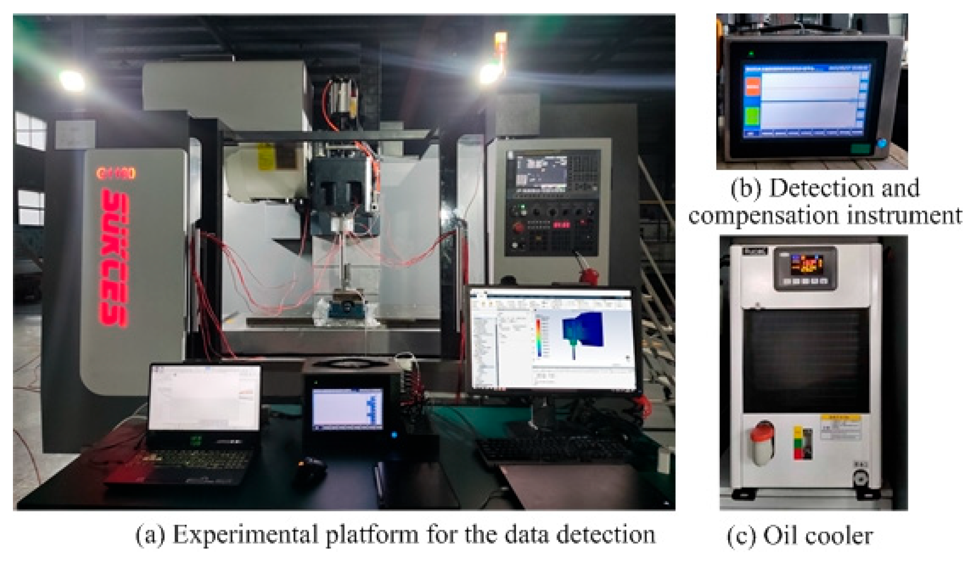
4. Experimental Platform Construction and Data Detection
5. The Solution of Thermal Characteristics Based on Multiple Time-Varying Factors
6. Analysis of Solution Results
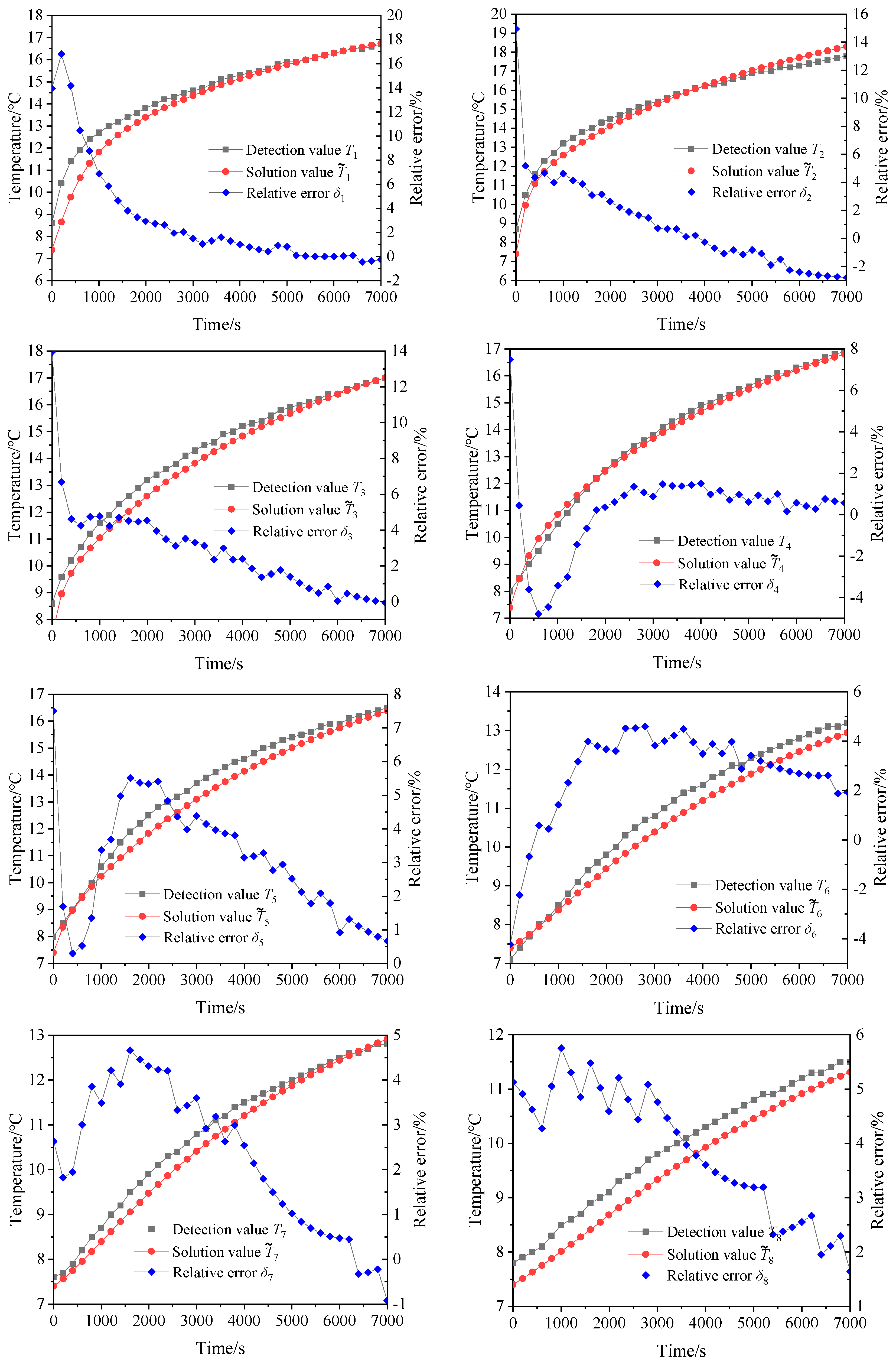
6.1. Temperature Analysis of Spindle System
6.2. Axial Displacement of the Spindle
7. Comparison of Thermal Characteristics Solution with Non Time-Varying Factors
8. Conclusions
Author Contributions
Funding
Data Availability Statement
Conflicts of Interest
References
- Liu, W.; Zhang, S.; Lin, J.; Xia, Y.; Wang, J.; Sun, Y. Advancements in accuracy decline mechanisms and accuracy retention approaches of CNC machine tools: A review. Int. J. Adv. Manuf. Technol. 2022, 121, 7087–7115. [Google Scholar] [CrossRef]
- Hu, X.; Zhao, Q.; Yang, Y.; Wan, S.; Sun, Y.; Hong, J. Accuracy analysis for machine tool spindles considering full parallel connections and form errors based on skin model shapes. J. Comput. Des. Eng. 2023, 10, 1970–1987. [Google Scholar] [CrossRef]
- Abele, E.; Altintas, Y.; Brecher, C. Machine tool spindle units. CIRP Ann.—Manuf. Technol. 2010, 59, 781–802. [Google Scholar] [CrossRef]
- Li, Y.; Zhao, W.; Lan, S.; Ni, J.; Wu, W.; Lu, B. A review on spindle thermal error compensation in machine tools. Int. J. Mach. Tools Manuf. 2015, 95, 20–38. [Google Scholar] [CrossRef]
- Mayr, J.; Jedrzejewski, J.; Uhlmann, E.; Donmez, M.A.; Knapp, W.; Härtig, F.; Wendt, K.; Moriwaki, T.; Shore, P.; Schmitt, R.; et al. Thermal issues in machine tools. CIRP Ann.—Manuf. Technol. 2012, 61, 771–791. [Google Scholar] [CrossRef]
- Lee, J.; Kim, D.-H.; Lee, C.-M. A study on the thermal characteristics and experiments of High-Speed spindle for machine tools. Int. J. Precis. Eng. Manuf. 2015, 16, 293–299. [Google Scholar] [CrossRef]
- Raja, V.P.; Moorthy, R.S. Prediction of Temperature Distribution of the Spindle System by Proposed Finite Volume and Element Method. Arab. J. Sci. Eng. 2019, 44, 5779–5785. [Google Scholar] [CrossRef]
- Mare, M.; Horej, O.; Nykodym, P. An Indicative Model Considering Part of the Thermo-Mechanical Behaviour of a Large Grinding Machine. In Proceedings of the 3rd International Conference on Thermal Issues in Machine Tools (ICTIMT2023): Lecture Notes in Production Engineering (LNPE), Dresden, Germany, 21–23 March 2023; Springer Nature: Cham, Switzerland, 2023; Volume F1165, pp. 54–66. [Google Scholar]
- Kaftan, P.; Mayr, J.; Wegener, K. Thermal Compensation of Sudden Working Space Condition Changes in Swiss-Type Lathe Machining. In Proceedings of the 3rd International Conference on Thermal Issues in Machine Tools (ICTIMT2023): Lecture Notes in Production Engineering (LNPE), Dresden, Germany, 21–23 March 2023; Springer Nature: Cham, Switzerland, 2023; Volume F1165, pp. 15–27. [Google Scholar]
- Than, V.T.; Huang, J.H. Nonlinear thermal effects on high-speed spindle bearings subjected to preload. Tribol. Int. 2016, 96, 361–372. [Google Scholar] [CrossRef]
- Liu, J.; Ma, C.; Wang, S.; Wang, S.; Yang, B.; Shi, H. Thermal-structure interaction characteristics of a high-speed spindle-bearing system. Int. J. Mach. Tools Manuf. 2019, 137, 42–57. [Google Scholar] [CrossRef]
- Xiang, S.T.; Yao, X.D.; Du, Z.C.; Yang, J.G. Dynamic linearization modeling approach for spindle thermal errors of machine tools. Mechatronics 2018, 53, 215–228. [Google Scholar] [CrossRef]
- Wu, L.; Tan, Q.C. Thermal Characteristic Analysis and Experimental Study of a Spindle-Bearing System. Entropy 2016, 18, 271. [Google Scholar] [CrossRef]
- Brecher, C.; Dehn, M.; Neus, S. A Data-Based Model of the Thermo-Elastic TCP Error Using the Encoder Difference and Neural Networks. In Proceedings of the 3rd International Conference on Thermal Issues in Machine Tools (ICTIMT2023): Lecture Notes in Production Engineering (LNPE), Dresden, Germany, 21–23 March 2023; Springer Nature: Cham, Switzerland, 2023; Volume F1165, pp. 119–131. [Google Scholar]
- Wenkler, E.; Steiert, C.; Boos, E.; Ihlenfeldt, S. Analysing the Impact of Process Dependent Thermal Loads on the Prediction Accuracy of Thermal Effects in Machine Tool Components. In Proceedings of the 3rd International Conference on Thermal Issues in Machine Tools (ICTIMT2023): Lecture Notes in Production Engineering (LNPE), Dresden, Germany, 21–23 March 2023; Springer Nature: Cham, Switzerland, 2023; Volume F1165, pp. 99–115. [Google Scholar]
- Ouyang, X.-L.; Xu, R.-N.; Jiang, P.-X. Three-equation local thermal non-equilibrium model for transient heat transfer in porous media: The internal thermal conduction effect in the solid phase. Int. J. Heat Mass Transf. 2017, 115, 1113–1124. [Google Scholar] [CrossRef]
- Wang, L.; Li, Y.; Marignetti, F.; Boglietti, A. Coupled Fluid-Solid Heat Transfer of A Gas and Liquid Cooling PMSM Including Rotor Rotation. IEEE Trans. Energy Convers. 2022, 37, 443–453. [Google Scholar] [CrossRef]
- Kang, C.M.; Zhao, C.Y.; Zhang, J.Q. Thermal behavior analysis and experimental study on the vertical machining center spindle. Trans. Can. Soc. Mech. Eng. 2020, 44, 344–351. [Google Scholar] [CrossRef]
- Kosarac, A.; Cep, R.; Trochta, M.; Knezev, M.; Zivkovic, A.; Mladjenovic, C.; Antic, A. Thermal Behavior Modeling Based on BP Neural Network in Keras Framework for Motorized Machine Tool Spindles. Materials 2022, 15, 7782. [Google Scholar] [CrossRef] [PubMed]
- Xu, C.; Zhang, J.F.; Wu, Z.J.; Yu, D.W.; Feng, P.F. Dynamic modeling and parameters identification of a spindle-holder taper joint. Int. J. Adv. Manuf. Technol. 2013, 67, 1517–1525. [Google Scholar] [CrossRef]
- Li, Y.; Zhang, Y.; Zhao, Y.; Shi, X. Thermal-mechanical coupling calculation method for deformation error of motorized spindle of machine tool. Eng. Fail. Anal. 2021, 128, 105597. [Google Scholar] [CrossRef]
- Zhang, J.F.; Feng, P.F.; Chen, C.; Yu, D.W.; Wu, Z.J. A method for thermal performance modeling and simulation of machine tools. Int. J. Adv. Manuf. Technol. 2013, 68, 1517–1527. [Google Scholar] [CrossRef]
- Basse, N.T. An Algebraic Non-Equilibrium Turbulence Model of the High Reynolds Number Transition Region. Water 2023, 15, 3234. [Google Scholar] [CrossRef]
- Chen, C. Study on Analysis and Optimization for Thermal Performance of Vertical Machining Center; Tsinghua University: Beijing, China, 2011. [Google Scholar]
- Zhu, K.; Shi, X.; Gao, J.; Li, F. Thermal Characteristics Analysis for a Motorized Spindle with Shaft Core Cooling Based on Numerical Simulation and Experimental Research. Hsi-An Chiao Tung Ta Hsueh/J. Xi’an Jiaotong Univ. 2018, 52, 40–47. [Google Scholar]
- Shi, X.; Kang, Y.; Fan, L.; Gao, J. Thermo-structural coupling calculation method for permanent magnetic synchronous motorized spindle. Huazhong Keji Daxue Xuebao (Ziran Kexue Ban)/J. Huazhong Univ. Sci. Technol. (Nat. Sci. Ed.) 2017, 45, 50–54, 60. [Google Scholar]
- Li, Z.; Liu, H.; Wu, Z. Thermal Characteristics of Motorized Spindle Under Contact Thermal Resistance and Thermally Induced Load. Modul. Mach. Tool Autom. Manuf. Tech. 2023, 6, 114–118. [Google Scholar]
- Pei, X.; Zhang, A.; Li, H.; Liu, M. Thermal deformation analysis of machine tool spindle system and experimental research. Mach. Des. Manuf. 2022, 6, 286–289, 294. [Google Scholar]
- Chen, X.; Quan, Y. Modern Practical Machine Tool Design Manual; China Machine Press: Beijing, China, 2006. [Google Scholar]
- Cui, L.; Zhang, D.; Gao, W.; Qi, X.; Shen, Y. Thermal errors simulation and modeling of motorized spindle. In Proceedings of the 2010 International Conference on Advances in Materials and Manufacturing Processes, ICAMMP 2010, Shenzhen, China, 6–8 November 2010; Trans Tech Publications: Stafa, Switzerland, 2011; Volume 154–155, pp. 1305–1309. [Google Scholar]
- Yin, Y.; Shi, D.; Fairchild, A.J. The Effect of Model Size on the Root Mean Square Error of Approximation (RMSEA): The Nonnormal Case. Struct. Equ. Model. 2023, 30, 378–392. [Google Scholar] [CrossRef]
- Bar-Gera, H. The Target Parameter of Adjusted R-Squared in Fixed-Design Experiments. Am. Stat. 2017, 71, 112–119. [Google Scholar] [CrossRef]
- Zhang, X.M.; Ren, Z.P.; Mei, F.M. Heat Transfer, 5th ed.; China Architecture & Building Press: Beijing, China, 2007; pp. 325–326. [Google Scholar]


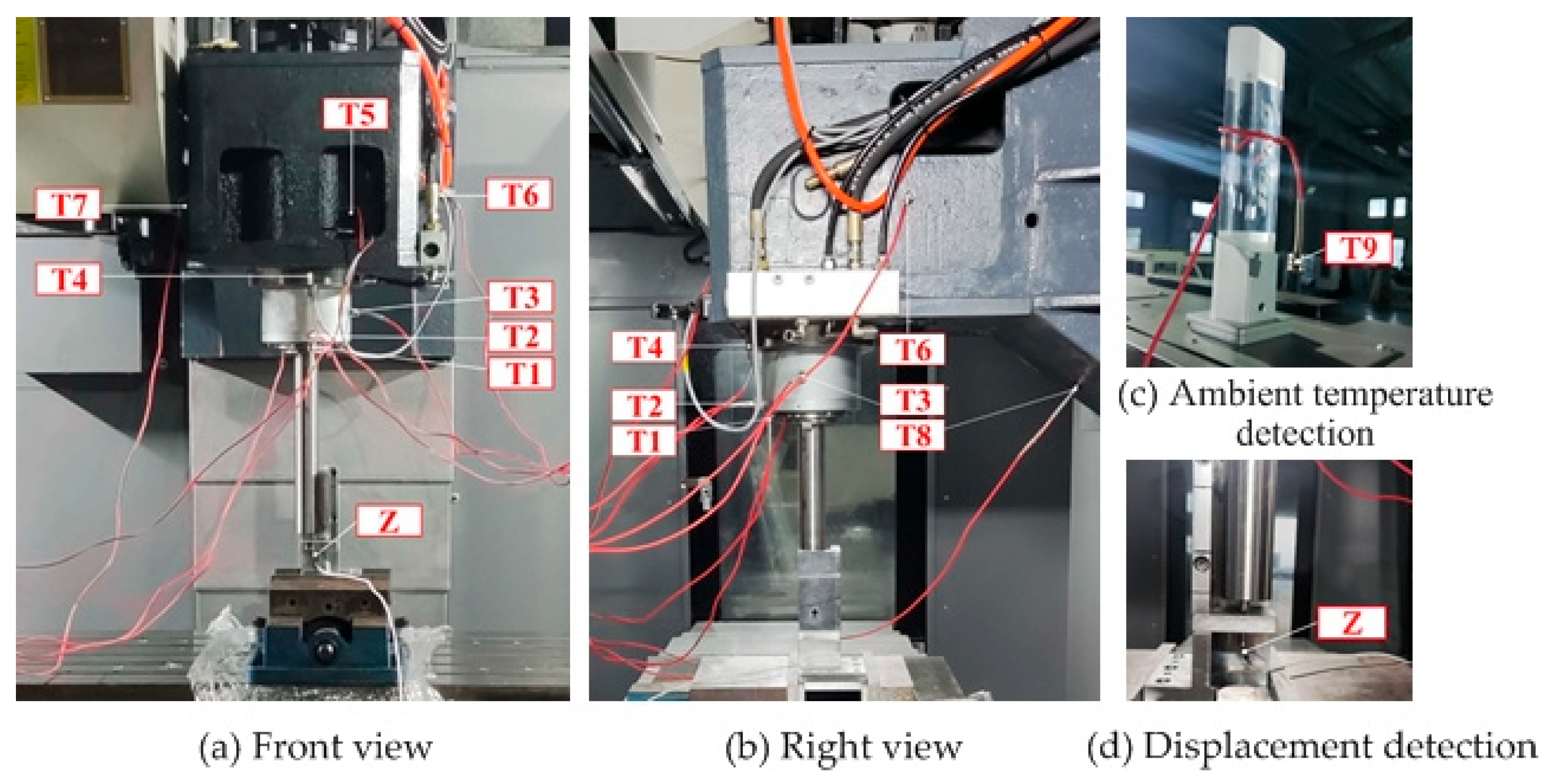
| Sensor Type | Sensor Position | Sensor Number |
|---|---|---|
| Temperature sensor | spindle end | T1, T2 |
| spindle bearings | T3 | |
| flange | T4 | |
| spindle body | T5 | |
| both sides of the spindle box | T6, T7 | |
| spindle box support plate | T8 | |
| ambient temperature | T9 | |
| Displacement sensor | inspection rod end | Z |
| Function | RMSE | R-Square |
|---|---|---|
| 0.9948 | 0.05874 | |
| 0.9997 | 0.04025 |
| Parameter | ρair | μair | Prair | λair |
|---|---|---|---|---|
| Sensitivity/% | 0.69 | 0.49 | 0.01 | 0.87 |
Disclaimer/Publisher’s Note: The statements, opinions and data contained in all publications are solely those of the individual author(s) and contributor(s) and not of MDPI and/or the editor(s). MDPI and/or the editor(s) disclaim responsibility for any injury to people or property resulting from any ideas, methods, instructions or products referred to in the content. |
© 2024 by the authors. Licensee MDPI, Basel, Switzerland. This article is an open access article distributed under the terms and conditions of the Creative Commons Attribution (CC BY) license (https://creativecommons.org/licenses/by/4.0/).
Share and Cite
Lin, X.; Deng, X.; Zheng, J.; Yao, X.; Shen, H. Thermal Characteristics of Spindle System Based on the Comprehensive Effect of Multiple Nonlinear Time-Varying Factors. Processes 2024, 12, 423. https://doi.org/10.3390/pr12020423
Lin X, Deng X, Zheng J, Yao X, Shen H. Thermal Characteristics of Spindle System Based on the Comprehensive Effect of Multiple Nonlinear Time-Varying Factors. Processes. 2024; 12(2):423. https://doi.org/10.3390/pr12020423
Chicago/Turabian StyleLin, Xiaoliang, Xiaolei Deng, Junjian Zheng, Xinhua Yao, and Hongyao Shen. 2024. "Thermal Characteristics of Spindle System Based on the Comprehensive Effect of Multiple Nonlinear Time-Varying Factors" Processes 12, no. 2: 423. https://doi.org/10.3390/pr12020423
APA StyleLin, X., Deng, X., Zheng, J., Yao, X., & Shen, H. (2024). Thermal Characteristics of Spindle System Based on the Comprehensive Effect of Multiple Nonlinear Time-Varying Factors. Processes, 12(2), 423. https://doi.org/10.3390/pr12020423