
An Improved Prediction Method for Failure Probability of Natural Gas Pipeline Based on Multi-Layer Bayesian Network


 ,
,  ,
,
Abstract
:1. Introduction
2. Bayesian Network Model of Gas Pipeline Failure Probability
3. Construction of the Bayesian Network Structure
- (1)
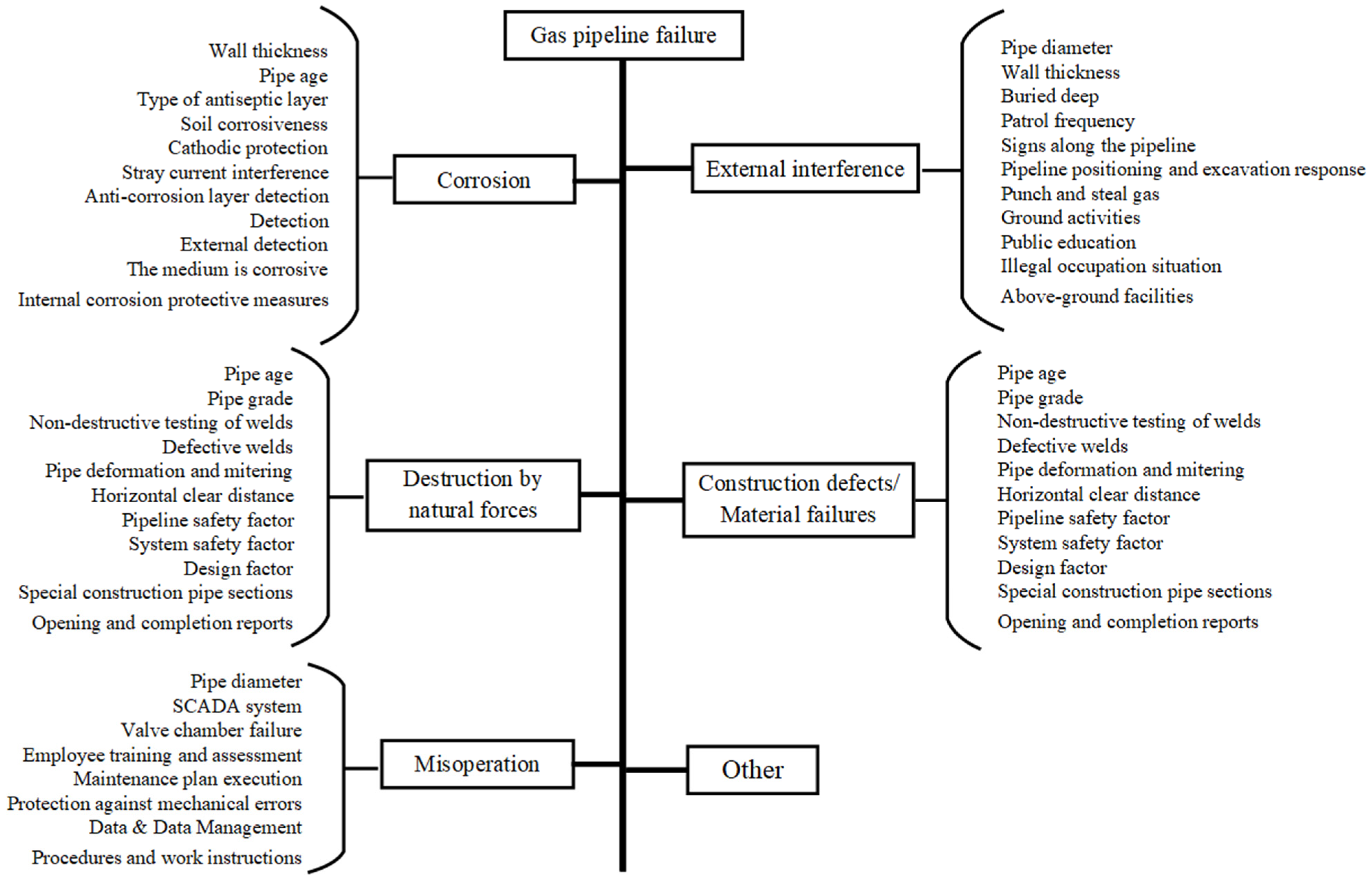
- In the failure factor tree map, the pipeline failure is mapped to the subnode, the failure causes are mapped to the intermediate node, and the impact factors are mapped to the parent nodes, and each node is labeled;
- (2)
- The function relationship in the failure factor dendrogram is mapped to the directed edge in the Bayesian network;
- (3)
- The state of the influencing factor is the prior probability of the node in the Bayesian network, and the function relationship between the nodes is the conditional probability of the edges in the Bayesian network.
4. Determination of Bayesian Network Parameters
4.1. Solution Procedure
- (1)
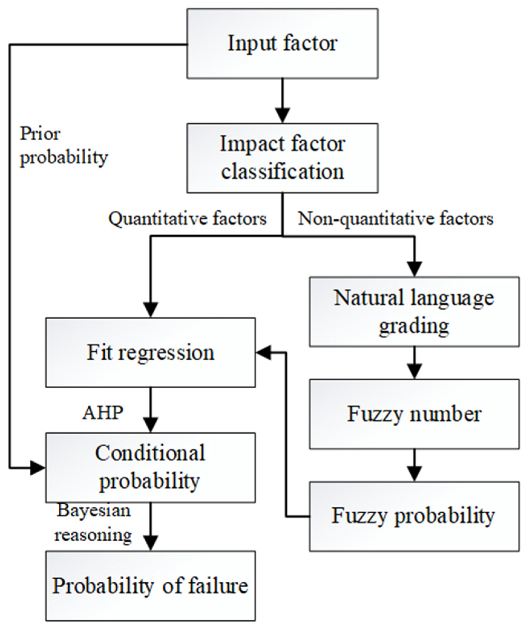
- Categorical impact factors: According to the nature of the impact factors and the difficulty of quantification, 51 impact factors were classified. Pipe diameter, wall thickness, buried depth, pipe age, anticorrosion layer type, and pipeline steel grade were the quantitative factors, which can directly quantify the function relationship between this factor and pipeline failure frequency, and the rest were nonquantitative factors.
- (2)
- The functional relationship between the impact factors and the pipeline failure frequency was quantified. For quantitative factors, the factors were fit as a function of the pipeline failure frequency; for nonquantitative factors, we referred to the relevant standard manuals [26,27,28,29,30] and the literature to divide the evaluation criteria of the impact factor and establish the membership function correspondence between the grade evaluation criteria and the fuzzy number [31]. We then converted the fuzzy number into fuzzy probability through Equations (2) and (3) and fit the function relationship between the fuzzy number and the fuzzy probability.
- (3)
- The conditional probabilities were calculated. The optimal fitting function was filtered, the median value of the fitting function was calculated, the median value judgment matrix was constructed, the maximum eigenvalue and the corresponding eigenvector of the matrix were calculated, and the conditional probability of the directed edge from the parent node to the subnode was calculated.
- (4)
- The pipeline prior probability was calculated. According to the pipeline parameters and the surrounding environment of the pipeline, the failure probability of the corresponding influencing factor in the parent node was calculated according to the optimal fitting function in step (2), which is the prior probability.
- (1)
- Based on a five-level natural language expression scale, namely “excellent”, “good”, “medium”, “poor” and “inferior”, the corresponding evaluation grades were “I”, “II”, “III”, “IV”, and “V”.
- (2)
- The quantization level was an ambiguous number. A link was established between rank and triangular fuzzy numbers [31,32], with grade I corresponding to 0.1, grade II corresponding to 0.3, grade III corresponding to 0.5, grade IV corresponding to 0.7, and grade V corresponding to 0.9. The fuzzy number was converted into fuzzy probability using Equations (2) and (3), and Table 1 shows the results after the transformation.
- (3)
- Fitting function relationships involved taking the fuzzy number as the independent variable and the fuzzy probability as the dependent variable; then, the function relationship between the fuzzy number and the fuzzy probability was fitted. Figure 6 shows the fuzzy probability corresponding to the fuzzy number of the interval [0, 1].
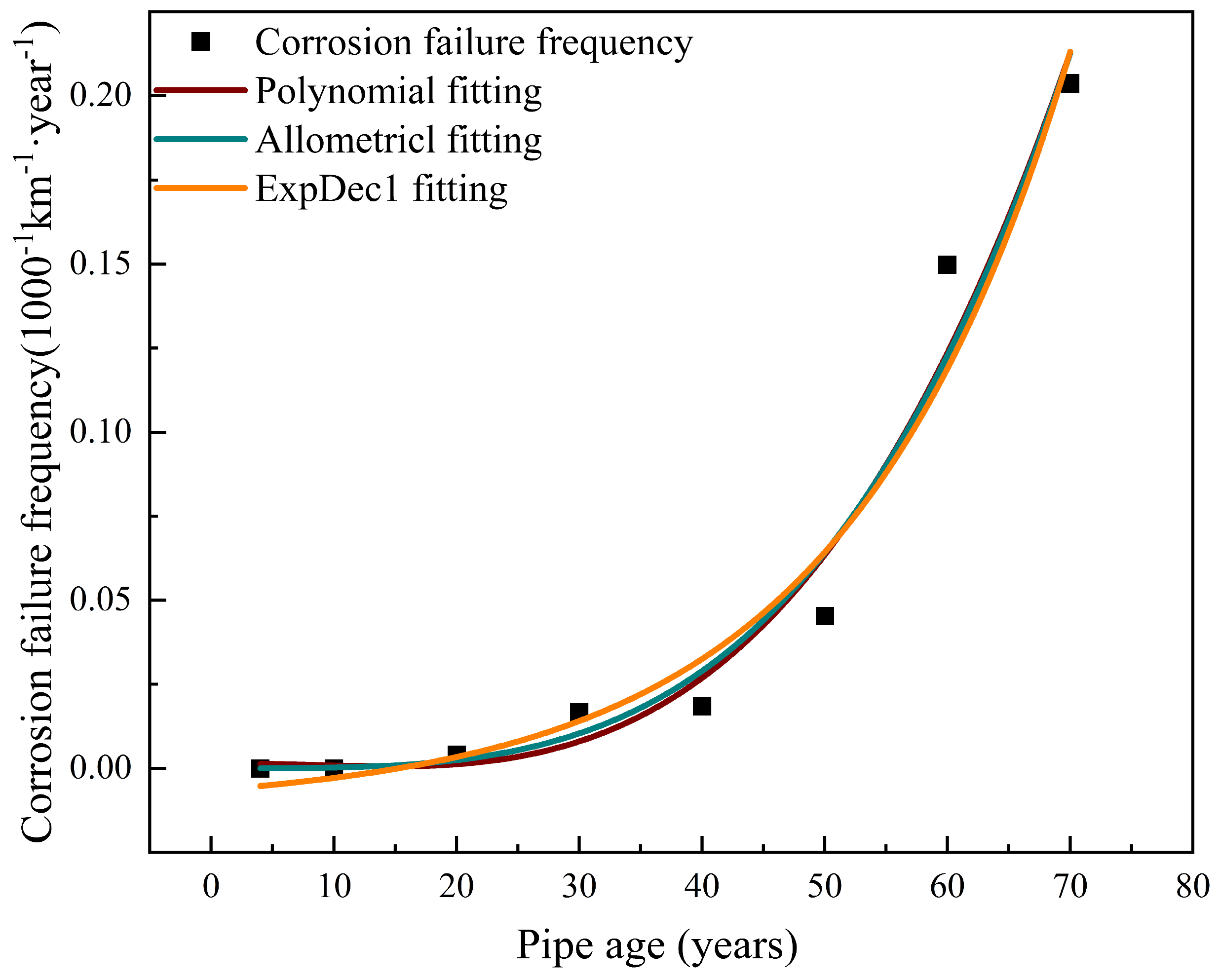
- (4)
- Based on the fitting results of the function relationship, the optimal fitting function was screened after a comprehensive analysis of the function characteristics, the rationality of the fitting function, and the goodness of fit (Table 2). Due to the discrete relationship between the steel grade and the type of anticorrosion layer and the failure frequency, it cannot be expressed by the fitting function, and the corresponding relationship between the influencing factor and the failure probability is shown in Table 3 and Table 4.
4.2. Calculation of Conditional Probabilities
- (1)
- The median value of the fitting function is calculated according to the integral median value theorem (Equation (4)).
- (2)
- A judgment matrix of the median value is constructed. If the node has n parent nodes, an n × n square matrix is established first, which is the judgment matrix. The values in row i, and column j in the matrix indicate the importance of the ith evaluation index relative to the jth evaluation index, as shown in Table 5.
- (3)
- The maximum eigenvalue λmax and the corresponding eigenvector ω of each judgment matrix are solved. The maximum eigenvalue λmax of the corrosion judgment matrix is 11, and the eigenvector ω is shown in Equation (5).
- (4)
- A consistency test is performed, and the judgment matrix is adjusted. According to the consistency ratio of the judgment matrix, the CR test judges whether the contradiction degree of the matrix is reasonable, and if the CR < 0.1, the consistency of the matrix is considered acceptable; otherwise, the matrix needs to be adjusted. Equations (6) and (7) are the formulas for testing the consistency of the matrix [33].
- (5)
- Assuming that the features are independent of each other, and the conditional probabilities between the features are also independent of each other in the case of a given category, Equation (8) is the conditional probability formula for calculating multiple parent nodes:
5. Examples of Application
6. Prior Probability
7. Bayesian Network Analysis
8. Conclusions
- (1)
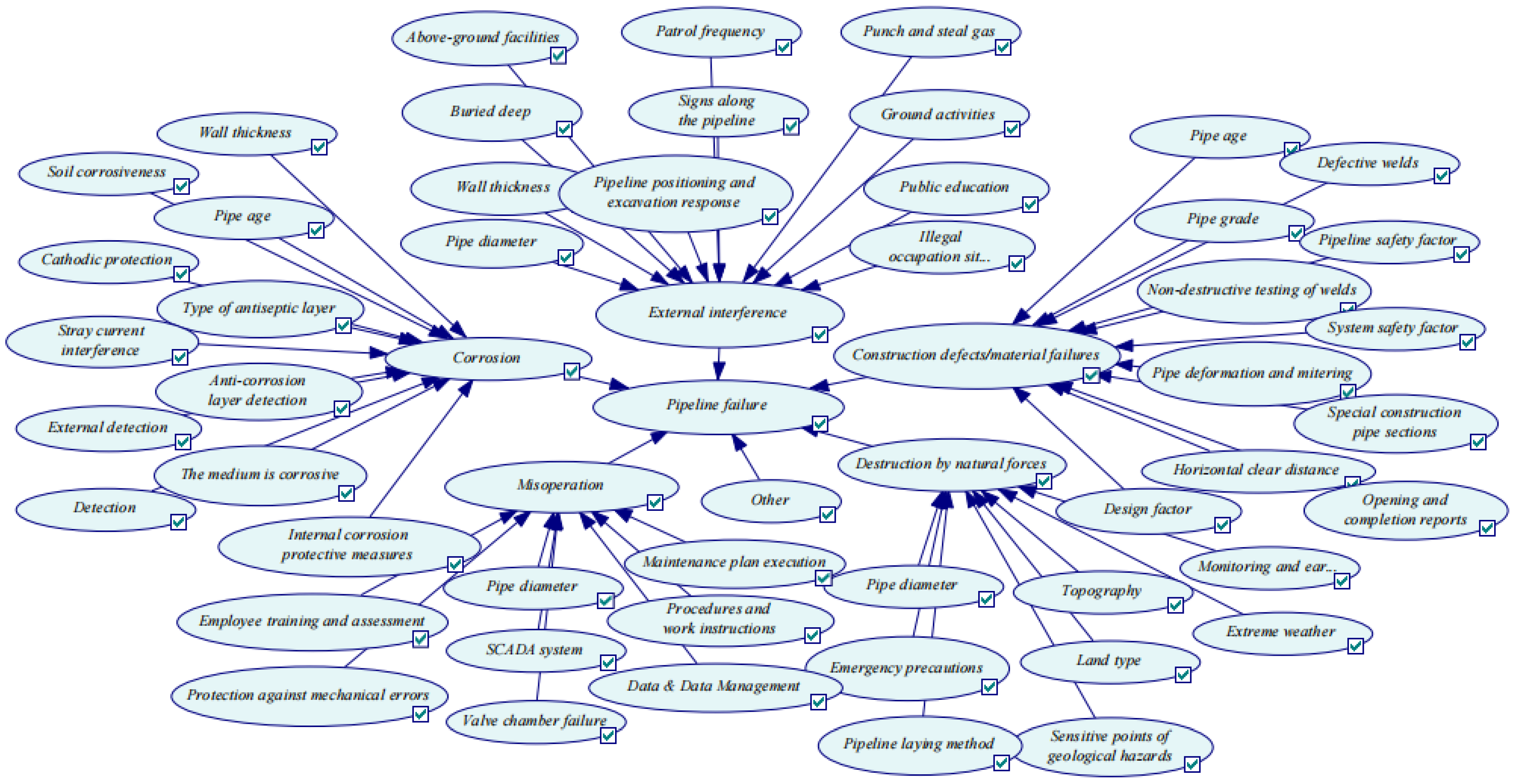
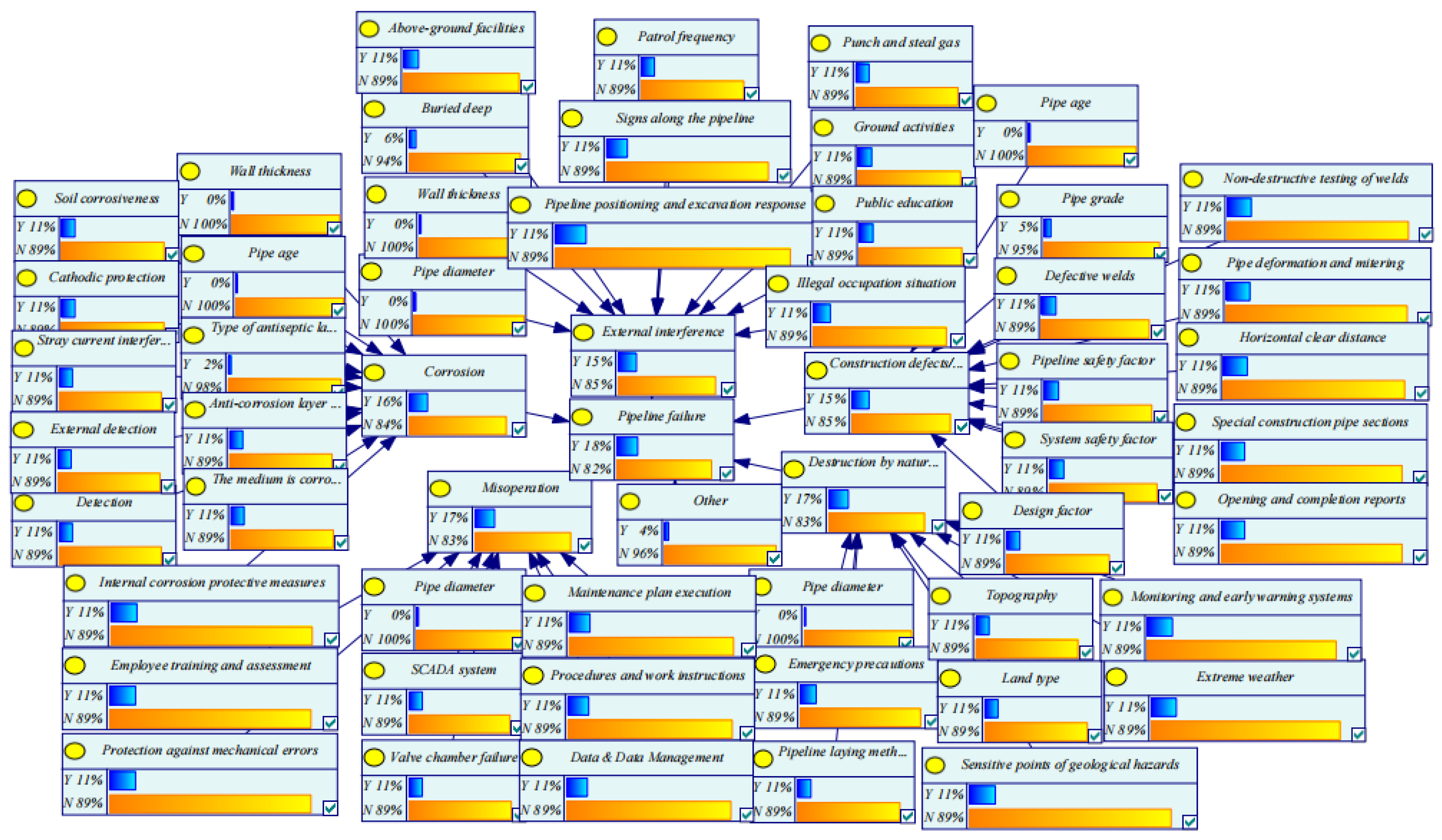
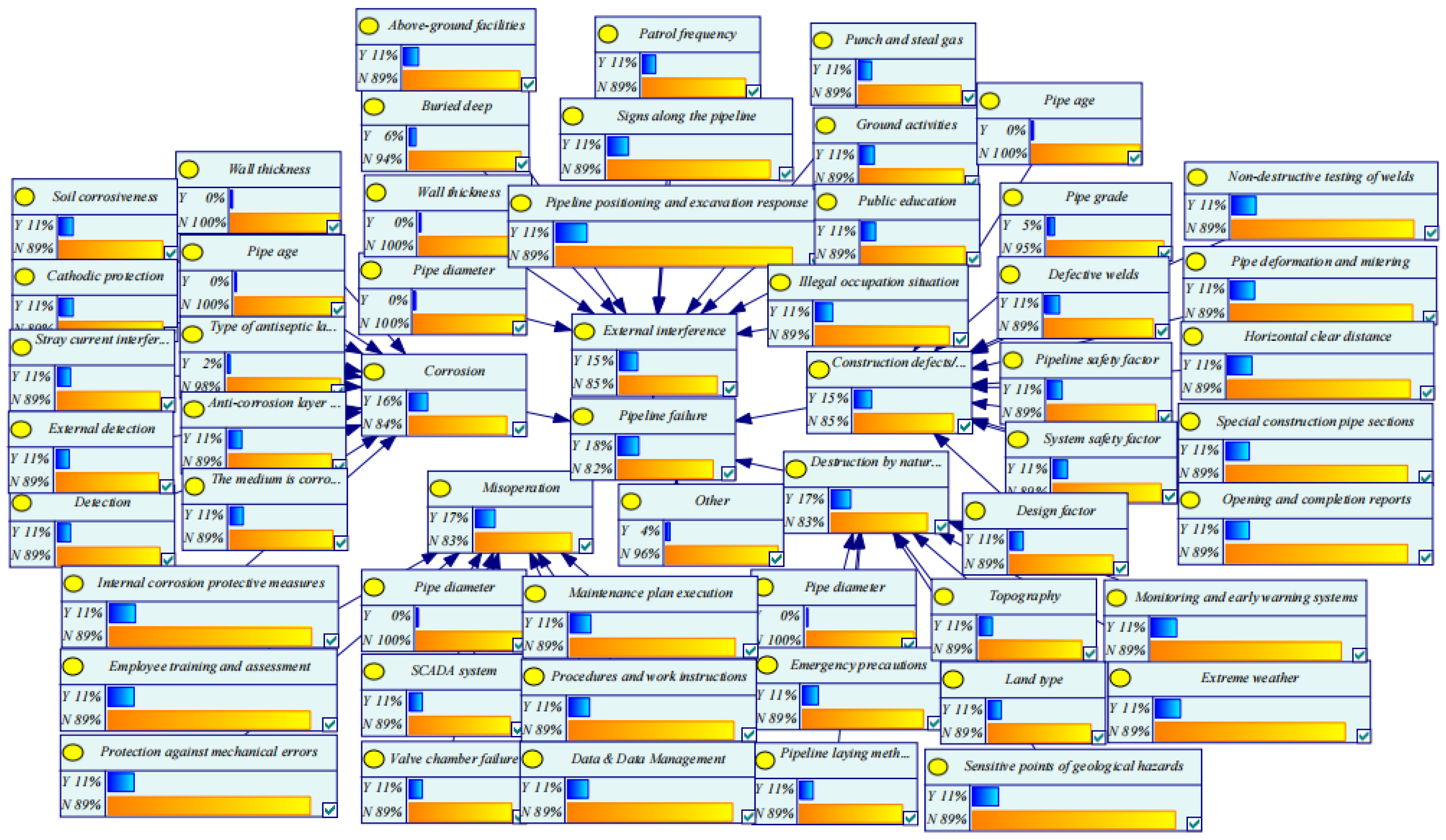
- According to the correspondence between the failure factor tree map and the Bayesian network, a three-layer Bayesian network topology model from the static failure factor tree map to the dynamic “pipeline failure–failure cause–influencing factor” was constructed with the pipeline as the subnode of the network, the type of pipeline failure as the intermediate node, and the factor affecting the pipeline failure as the parent node.
- (2)
- The optimal fitting function between the influencing factor and the pipeline failure frequency was screened, the median value of the fitting function integral was proposed as the data basis, and the conditional probability of the directed edge of the network was calculated by constructing the judgment matrix of the median value and solving the maximum eigenvalue and eigenvector of the matrix.
- (3)
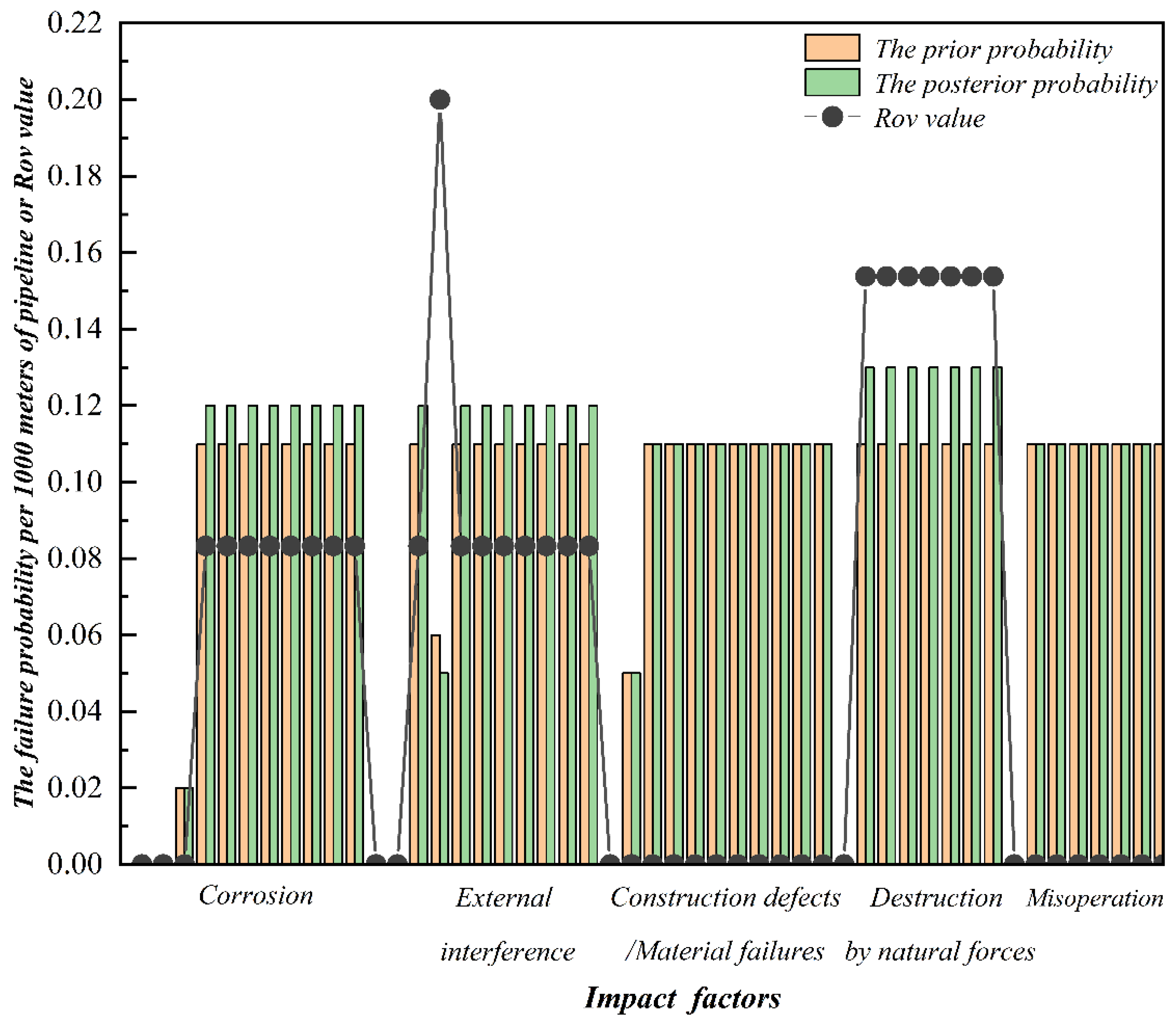
- In the Bayesian network model, the prior probability of the pipeline was calculated by inputting the fuzzy number of pipeline parameters and pipeline operation and maintenance information into the optimal fitting function. Forward reasoning involves calculating the likelihood of pipeline failure, and reverse reasoning highlights the significance of the impact factor of pipeline failure and offers reference data for key protections and precise positioning of pipeline-related departments.
- (1)
- The applicability and uncertainty of failure data samples from PHMSA and EGIG about other pipelines;
- (2)
- The challenge of integrating failure data for a pipeline that has missing data for a certain period, specifically, how to incorporate these data into the existing method.
Author Contributions
Funding
Data Availability Statement
Conflicts of Interest
References
- BBC. What Caused the Blast That Destroyed a Girls’ School—BBC News 2020. Available online: https://www.bbc.co.uk/news/video_and_audio/headlines/54208394/lagos-inferno-what-caused-the-blast-that-destroyed-a-nigerian-girls-school (accessed on 14 October 2020).
- Carlson, L.C.; Rogers, T.T.; Kamara, T.B.; Rybarczyk, M.M.; Leow, J.J.; Kirsch, T.D.; Kushner, A.L. Petroleum pipeline explosions in sub-Saharan Africa: A comprehensive systematic review of the academic and lay literature. Burns 2015, 41, 497–501. [Google Scholar] [CrossRef]
- Wu, W.; Li, Y.; Cheng, G.; Zhang, H.; Kang, J. Dynamic safety assessment of oil and gas pipeline containing internal corrosion defect using probability theory and possibility theory. Eng. Fail. Anal. 2019, 98, 156–166. [Google Scholar] [CrossRef]
- Hassan, S.; Wang, J.; Kontovas, C.; Bashir, M. An assessment of causes and failure likelihood of cross-country pipelines under uncertainty using Bayesian networks. Reliab. Eng. Syst. Saf. 2022, 218, 108171. [Google Scholar] [CrossRef]
- Shan, K.; Shuai, J.; Xu, K.; Zheng, W. Failure probability assessment of gas transmission pipelines based on historical failure-related data and modification factors. J. Nat. Gas Sci. Eng. 2018, 52, 356–366. [Google Scholar] [CrossRef]
- Vianello, C.; Maschio, G. Quantitative risk assessment of the Italian gas distribution network. J. Loss Prev. Process Ind. 2014, 32, 5–17. [Google Scholar] [CrossRef]
- Xiang, W.; Zhou, W. Bayesian network model for predicting probability of third-party damage to underground pipelines and learning model parameters from incomplete datasets. Reliab. Eng. Syst. Saf. 2021, 205, 107262. [Google Scholar] [CrossRef]
- Witek, M. Gas transmission pipeline failure probability estimation and defect repairs activities based on in-line inspection data. Eng. Fail. Anal. 2016, 70, 255–272. [Google Scholar] [CrossRef]
- Ferdous, R.; Khan, F.; Sadiq, R.; Amyotte, P.; Veitch, B. Analyzing system safety and risks under uncertainty using a bow-tie diagram: An innovative approach. Process Saf. Environ. Prot. 2013, 91, 1–18. [Google Scholar] [CrossRef]
- Khakzad, N.; Khan, F.; Amyotte, P. Safety analysis in process facilities: Comparison of fault tree and Bayesian network approaches. Reliab. Eng. Syst. Saf. 2011, 96, 925–932. [Google Scholar] [CrossRef]
- Badida, Y. Risk evaluation of oil and natural gas pipelines due to natural hazards using fuzzy fault tree analysis. J. Nat. Gas Sci. Eng. 2019, 66, 284–292. [Google Scholar] [CrossRef]
- Zarei, E.; Azadeh, A.; Khakzad, N.; Aliabadi, M.M.; Mohammadfam, I. Dynamic safety assessment of natural gas stations using Bayesian network. J. Hazard. Mater. 2017, 321, 830–840. [Google Scholar] [CrossRef]
- Hong, B.; Shao, B.; Guo, J.; Fu, J.; Li, C.; Zhu, B. Dynamic Bayesian network risk probability evolution for third-party damage of natural gas pipelines. Appl. Energy 2023, 333, 120620. [Google Scholar] [CrossRef]
- Yin, B.; Li, B.; Liu, G.; Wang, Z.; Sun, B. Quantitative risk analysis of offshore well blowout using Bayesian network. Saf. Sci. 2021, 135, 105080. [Google Scholar] [CrossRef]
- Wang, Q.; Li, C. Evaluating risk propagation in renewable energy incidents using ontology-based Bayesian networks extracted from news reports. Int. J. Green Energy 2021, 19, 1290–1305. [Google Scholar] [CrossRef]
- Carless, T.S.; Redus, K.; Dryden, R. Estimating nuclear proliferation and security risks in emerging markets using Bayesian Belief Networks. Energy Pol. 2021, 159, 112549. [Google Scholar] [CrossRef]
- Li, F.; Wang, W.; Dubljevic, S.; Khan, F.; Xu, J.; Yi, J. Analysis on accident-causing factors of urban buried gas pipeline network by combining DEMATEL, ISM and BN methods. J. Loss Prev. Process Ind. 2019, 61, 49–57. [Google Scholar] [CrossRef]
- Fakhravar, D.; Khakzad, N.; Reniers, G.; Cozzani, V. Security vulnerability assessment of gas pipeline using Bayesian network. In Proceedings of the 27th European Safety and Reliability Conference, ESREL 2017, Portorož, Slovenia, 18–22 June 2017. [Google Scholar]
- Wu, J.; Zhou, R.; Xu, S.; Wu, Z. Probabilistic analysis of natural gas pipeline network accident based on Bayesian network. J. Loss Prev. Process Ind. 2017, 46, 126–136. [Google Scholar] [CrossRef]
- Chin, K.-S.; Tang, D.-W.; Yang, J.-B.; Wong, S.Y.; Wang, H. Assessing new product development project risk by Bayesian network with a systematic probability generation methodology. Expert Syst. Appl. 2009, 36, 9879–9890. [Google Scholar] [CrossRef]
- Zhao, M. About the Bayes formula and its practical application. Sci. Technol. Innov. 2023, 18, 0067-04. [Google Scholar]
- Li, X.H.; Guo, M.; Zhu, H. Quantitative risk analysis on leakage failure of submarine oil and gas pipelines using Bayesian network. Process Saf. Environ. Prot. 2016, 103 Pt A, 163–173. [Google Scholar] [CrossRef]
- Cui, Y.; Quddus, N.; Mashuga, C.V. Bayesian Network and Game Theory Risk Assessment Model for Third-Party Damage to Oil and Gas Pipelines. Process Saf. Environ. Prot. 2020, 134, 178–188. [Google Scholar] [CrossRef]
- European Gas Pipeline Incident Report Group. 11th Report of the European Gas Pipeline Incident Group 1970–2019; EGIGL: Putten, The Netherlands, 2019; pp. 1–56. [Google Scholar]
- Feng, X.; Jiang, J.; Wang, W. Gas pipeline failure evaluation method based on a NoisyOR gate Bayesian network. J. Loss Prev. Process Ind. 2020, 66, 104175. [Google Scholar] [CrossRef]
- Ke, S.; Jian, S. Statistical analyses of incidents on oil and gas pipelines based on comparing different pipeline incident databases. In Proceedings of the ASME 2017 Pressure Vessels and Piping Conference, Waikoloa, HI, USA, 16–20 July 2017. [Google Scholar] [CrossRef]
- Muhlbauer, W.K. Pipeline Risk Management Manual: Ideas, Techniques, and Resources; Gulf Professional Publishing: Burlington, NJ, USA, 2004. [Google Scholar]
- SY/T 6891.1-2012; Oil & Gas Pipeline Risk Assessment Methods—Part 1: Semi-Quantitative Risk Assessment Method. Standards Press of China: Beijing, China, 2012.
- Det Norske Veritas. Recommended Practice DNV-RP-F107, Risk Assessment of Pipeline Protection; Det Norske Veritas: Oslo, Norway, 2019. [Google Scholar]
- SY/T 6828-2011; Technical Specification for Geological Hazards Risk Management of Oil and Gas Pipeline. Standards Press of China: Beijing, China, 2011.
- Onisawa, T. An approach to human reliability in man-machine systems using error possibility. Fuzzy Sets Syst. 1988, 27, 87–103. [Google Scholar] [CrossRef]
- Yuhua, D.; Datao, Y. Estimation of failure probability of oil and gas transmission pipelines by fuzzy fault tree analysis. J. Loss Prev. Process Ind. 2005, 18, 83–88. [Google Scholar] [CrossRef]
- Meng, X.; Chen, G.; Zhu, G.; Zhu, Y. Dynamic quantitative risk assessment of accidents induced by leakage on offshore platforms using DEMATEL-BN. Int. J. Nav. Archit. Ocean. Eng. 2018, 11, 22–32. [Google Scholar] [CrossRef]


| Impact Factor Rating | Fuzzy Number | Fuzzy Possibility (km−1·year−1) |
|---|---|---|
| I | 0.1 | 5.62 × 10⁻¹¹ |
| II | 0.3 | 2.88 × 10⁻⁷ |
| III | 0.5 | 1.17 × 10⁻⁵ |
| IV | 0.7 | 1.91 × 10⁻⁴ |
| V | 0.9 | 4.27 × 10⁻³ |
| Reason for Invalidation | Impact Factor | Judging Criteria | Optimal Fitting Function |
|---|---|---|---|
| Corrosion | Wall thickness | Fitting function | y = 9.23x−2.07 |
| Pipe age | Fitting function | y = 5.66 × 10−8x3.56 | |
| Type of antiseptic layer | Discrete relationships | / | |
| External interference | Pipe diameter | Fitting function | y = 2.66 × 10⁻³ + 0.99e−x/147.05 |
| Wall thickness | Fitting function | y = 8.68 × 10⁻⁴ + 5.82e−x/1.84 | |
| Buried deep | Fitting function | y = 5.71 × 10⁻² + 4.67e−x/22.67 | |
| Destruction by natural forces | Pipe diameter | Fitting function | y = 5.43 × 10−7x2.87 |
| Construction defects/material failures | Construction—Pipe age | Fitting function | y = 1.20 × 10−7x3.07 |
| Material—Pipe age | Fitting function | y = −7.38 × 10⁻³ + 0.066e−x/596.56 | |
| Pipe steel grade | Discrete relationships | / | |
| Misoperation | Pipe diameter | Fitting function | y = 127.90x−1.65 |
| Fuzzy number and fuzzy probability | y = −4.41 × 10⁻⁴ + 5.62 × 10⁻⁴ex/0.17 | ||
| Steel Grade | Failure Frequency (1000−1 km−1·year−1) |
|---|---|
| Grade A | 0.04221 |
| Grade B | 0.01587 |
| X42 | 0.01356 |
| X46 | 0.02583 |
| X52 | 0.02873 |
| X56 | 0.01392 |
| X60 | 0.00616 |
| X65 | 0.00409 |
| X70 and above | 0.04975 |
| Type of Antiseptic Layer | Failure Frequency (1000−1 km−1·year−1) |
| Coal tar | 0.04286 |
| Bitumen | 0.07 |
| Polyethylene | 0.00819 |
| Epoxy resin | 0.01959 |
| Other | 0.0855 |
| a11 | a12 | a13 | … | aij | |
|---|---|---|---|---|---|
| a11 | a11/a11 | a11/a12 | a11/a13 | … | a11/aij |
| a21 | a21/a11 | a21/a12 | a21/a13 | … | a21/aij |
| a31 | a31/a11 | a31/a12 | a31/a13 | … | a31/aij |
| … | … | … | … | … | … |
| aij | aij/a11 | aij/a12 | aij/a13 | … | aij/aij |
| n | 1 | 2 | 3 | 4 | 5 | 6 | 7 | 8 | 9 | 10 | 11 | 12 |
|---|---|---|---|---|---|---|---|---|---|---|---|---|
| RI | 0 | 0 | 0.52 | 0.89 | 1.12 | 1.26 | 1.36 | 1.41 | 1.46 | 1.49 | 1.52 | 1.54 |
| Corrosion | External Interference | Construction Defects/Material Failures | |||
|---|---|---|---|---|---|
| Impact Factor | Prior Probability (1000−1 km−1·Year−1) | Impact Factor | Prior Probability (1000−1 km−1·Year−1) | Impact Factor | Prior Probability (1000−1 km−1·Year−1) |
| Wall thickness | 9.47 × 10⁻⁴ | Pipe diameter | 2.91 × 10⁻³ | Pipe age | 2.72 × 10⁻⁴ |
| Pipe age | 2.07 × 10⁻⁴ | Wall thickness | 8.68 × 10⁻⁴ | Pipe grade | 4.98 × 10⁻² |
| Type of antiseptic layer | 1.96 × 10⁻² | Buried deep | 5.71 × 10⁻² | Non-destructive testing of welds | 1.13 × 10⁻¹ |
| Soil corrosiveness | 1.13 × 10⁻¹ | Patrol frequency | 1.13 × 10⁻¹ | Defective welds | 1.13 × 10⁻¹ |
| Cathodic protection | 1.13 × 10⁻¹ | Signs along the pipeline | 1.13 × 10⁻¹ | Pipe deformation and mitering | 1.13 × 10⁻¹ |
| Stray current interference | 1.13 × 10⁻¹ | Pipeline positioning and excavation response | 1.13 × 10⁻¹ | Horizontal clear distance | 1.13 × 10⁻¹ |
| Anticorrosion layer detection | 1.13 × 10⁻¹ | Punch and steal gas | 1.13 × 10⁻¹ | Pipeline safety factor | 1.13 × 10⁻¹ |
| Detection | 1.13 × 10⁻¹ | Ground activities | 1.13 × 10⁻¹ | System safety factor | 1.13 × 10⁻¹ |
| External detection | 1.13 × 10⁻¹ | Public Education | 1.13 × 10⁻¹ | Design factor | 1.13 × 10⁻¹ |
| The medium is corrosive | 1.13 × 10⁻¹ | Illegal occupation situation | 1.13 × 10⁻¹ | Special construction pipe sections | 1.13 × 10⁻¹ |
| Internal corrosion protective measures | 1.13 × 10⁻¹ | Above-ground facilities | 1.13 × 10⁻¹ | Opening and completion reports | 1.13 × 10⁻¹ |
| Destruction by Natural Forces | Misoperation | ||
|---|---|---|---|
| Impact Factor | Prior Probability (1000−1 km−1·year−1) | Impact Factor | Prior Probability (1000−1 km−1·year−1) |
| Pipe diameter | 3.51 × 10⁻⁴ | Pipe diameter | 1.05 × 10⁻³ |
| Topography | 1.13 × 10⁻¹ | SCADA system | 1.13 × 10⁻¹ |
| Land type | 1.13 × 10⁻¹ | Valve chamber failure | 1.13 × 10⁻¹ |
| Sensitive points of geological hazards | 1.13 × 10⁻¹ | Employee training and assessment | 1.13 × 10⁻¹ |
| Pipeline laying method | 1.13 × 10⁻¹ | Maintenance plan execution | 1.13 × 10⁻¹ |
| Extreme weather | 1.13 × 10⁻¹ | Protection against mechanical errors | 1.13 × 10⁻¹ |
| Monitoring and early warning systems | 1.13 × 10⁻¹ | Data and Data Management | 1.13 × 10⁻¹ |
| Emergency precautions | 1.13 × 10⁻¹ | Procedures and work instructions | 1.13 × 10⁻¹ |
Disclaimer/Publisher’s Note: The statements, opinions and data contained in all publications are solely those of the individual author(s) and contributor(s) and not of MDPI and/or the editor(s). MDPI and/or the editor(s) disclaim responsibility for any injury to people or property resulting from any ideas, methods, instructions or products referred to in the content. |
© 2024 by the authors. Licensee MDPI, Basel, Switzerland. This article is an open access article distributed under the terms and conditions of the Creative Commons Attribution (CC BY) license (https://creativecommons.org/licenses/by/4.0/).
Share and Cite
Weng, Y.; Sun, X.; Yang, Y.; Tao, M.; Liu, X.; Zhang, H.; Zhang, Q. An Improved Prediction Method for Failure Probability of Natural Gas Pipeline Based on Multi-Layer Bayesian Network. Processes 2024, 12, 2930. https://doi.org/10.3390/pr12122930
Weng Y, Sun X, Yang Y, Tao M, Liu X, Zhang H, Zhang Q. An Improved Prediction Method for Failure Probability of Natural Gas Pipeline Based on Multi-Layer Bayesian Network. Processes. 2024; 12(12):2930. https://doi.org/10.3390/pr12122930
Chicago/Turabian StyleWeng, Yueyue, Xu Sun, Yufeng Yang, Mengmeng Tao, Xiaoben Liu, Hong Zhang, and Qiang Zhang. 2024. "An Improved Prediction Method for Failure Probability of Natural Gas Pipeline Based on Multi-Layer Bayesian Network" Processes 12, no. 12: 2930. https://doi.org/10.3390/pr12122930
APA StyleWeng, Y., Sun, X., Yang, Y., Tao, M., Liu, X., Zhang, H., & Zhang, Q. (2024). An Improved Prediction Method for Failure Probability of Natural Gas Pipeline Based on Multi-Layer Bayesian Network. Processes, 12(12), 2930. https://doi.org/10.3390/pr12122930