Observer Design for State and Parameter Estimation for Two-Time-Scale Nonlinear Systems

Abstract

The design and calculation of nonlinear observers for parameter estimation in multi-time-scale nonlinear systems present significant challenges due to the inherent complexity and stiffness of such systems. This study proposes a framework for designing observers for two-time-scale nonlinear systems, with the objective of overcoming the aforementioned challenges. The design procedure involves reducing the original two-time-scale nonlinear system to a lower-dimensional model that captures only the slow dynamics while approximating the fast states through the use of an algebraic slow motion invariant manifold function. Subsequently, an exponential observer can be devised for this reduced system, which is valid for both state and parameter estimation. By employing the output from the original system, this observer can be adapted for online state and parameter estimation for the detailed two-time-scale system. The challenges associated with estimating parameters in two-time-scale nonlinear systems, the complexities of designing observers for such systems, and the computational burden associated with computing observers for ill-conditioned systems can be effectively addressed through the application of this design framework. A rigorous error analysis validates the convergence of the proposed observer towards the states and parameters of the original system. The viability and necessity of this observer design framework are demonstrated through a numerical example and an anaerobic digestion process. This study presents a practical approach for state and parameter estimation with observers for two-time-scale nonlinear systems.

1. Introduction

In a multitude of practical applications, model parameters that are essential for understanding system behavior and for controlling the system may be unmeasurable or change due to varying conditions. While sensors can provide insights into these parameters, their utilization is frequently neither feasible nor cost-effective. It is therefore essential to update the system model parameters through estimation in order to ensure optimal performance and stability. Over the past few decades, a variety of parameter estimation methods have been investigated, including the least squares method [1,2,3], Kalman filter techniques [4,5], and observer-based parameter identification [6,7,8]. Among these, the observer-based parameter estimation approach transforms the traditional state reconstruction problem into an online parameter estimation problem, thereby providing stable, accurate parameter estimates and allowing for dynamic adjustments based on real-time system conditions. In recent years, both theoretical and applied research on state and parameter observers for nonlinear systems has received increasing attention [9,10,11,12]. Backi et al. [13] employed an extended Kalman filter and a Monte Carlo-inspired approach. This method is effective at estimating state and parameter values in an offline situation. Afri et al. [14] employed a nonlinear Luenberger observer method to estimate the system state and parameters. Liu et al. [15] integrate the results of sensitivity analysis and variable selection into the MHE framework to achieve simultaneous estimation of the system state and parameters. Yin et al. [12] utilize a distributed extended Kalman filter and distributed mobile time-domain estimation to simultaneously study the system state and parameters.

As the number of states and parameters in control systems continues to grow, it has become increasingly common for systems to exhibit the property of multiple time scales [16]. To illustrate, in chemical and biological engineering systems, significant differences in reaction dynamics may result in the emergence of dynamic systems comprising both fast and slow modes. This discrepancy renders the design of an observer that aligns with the dynamics of the corresponding time-scaled system a challenging task [17]. Furthermore, the stiffness of these systems presents a significant challenge in the development and calculation of observers. In practice, the stiffness of the model can give rise to ill-conditioned control problems and hinder the attainment of convergence in state estimation [18].

In order to address these challenges, a common strategy is to employ model reduction techniques [19,20,21,22,23,24,25,26,27,28] with the objective of simplifying the system. The goal is to ensure that the time scales of the state dynamics in the reduced-order system are consistent while maintaining as much of the original system’s characteristics as possible.

A review of the literature reveals a notable absence of studies that adequately address the problem of state and parameter estimation for two-time-scale systems. Hooshmand et al. [29] study multi-time-scale systems using singular regression methods, i.e., ignoring the dynamics of the fast states by choosing appropriately small parameters. Farza et al. [30] employ extended high-gain observers to estimate the states as well as some unknown parameters. However, the singular perturbation approach neglects the fast process dynamics and can generate non-vanishing errors that are higher-order functions of the small parameters, whose accuracy is contingent upon the small parameters. The high-gain observer considers only fast eigenvalues, which results in a system that is highly sensitive to the measurement noise when studying slow subsystems. It is noteworthy that the slow-motion invariant manifold method stands out as a significant approach within the context of model reduction techniques. This approach constrains the system dynamics to the slow invariant manifold, thereby ensuring exponential asymptotic convergence of the reduced-order model [31]. In our previous research [17], this approach has been employed to simplify the design of a state observer for two-time-scale systems, thereby enabling precise state estimation. Nevertheless, the estimation of unknown parameters has yet to be addressed.

This work proposes a state and parameter observer design framework for two-time-scale nonlinear systems. The slow-motion invariant manifold method is employed to simplify the system dynamics, thereby circumventing the aforementioned issues. The observer design method presented in this paper addresses the challenges of high stiffness in solving the parameter estimation problem for two-time-scale nonlinear systems, the complexity of designing observers for two-time-scale systems, and the complexities of calculations involved in designing observers for high-dimensional models. The effectiveness of this methodology is illustrated through a rigorous error convergence analysis and numerical and anaerobic digestion case studies, thereby demonstrating the necessity and viability of the proposed observer design approach.

The paper is organized as follows: Section 2 introduces the model reduction method via slow-motion invariant manifolds. Section 3 outlines the design methodology of the observer for two-time-scale systems. Section 4 demonstrates the application through numerical simulations and a case study of the anaerobic digestion process. Section 5 concludes by summarizing the findings.

2. Preliminaries

Consider a nonlinear autonomous system of general form:

$$\left\{\begin{array}{c}{\displaystyle \frac{d\mathit{x}}{dt}}=\mathit{f}(\mathit{x})\\ \mathit{y}=\mathit{h}(\mathit{x})\end{array}\right.$$

(1)

where $\mathit{x}\in {\mathit{R}}^n$ and $\mathit{y}\in {\mathit{R}}^m$ are the state and output variables, $\mathit{f}(\mathit{x}):{\mathit{R}}^n\to {\mathit{R}}^n$ and $\mathit{h}(\mathit{x}):{\mathit{R}}^n\to {\mathit{R}}^m$ are real analytic vector functions. Furthermore, the nonlinear system satisfies the following assumptions:

Assumption 1.

The origin is an equilibrium point of the nonlinear system (1). The system can be locally linearized at the origin with a Jacobian matrix of $\mathit{F}={\displaystyle \frac{\partial \mathit{f}}{\partial \mathit{x}}}(0)$ and all eigenvalues of F have negative real parts, which ensures that the system is locally asymptotically stable near the origin.

Assumption 2.

The nonlinear system (1) exhibits two distinct time scales, i.e., the eigenvalues of the Jacobian matrix F can be divided into a “fast” subset of cardinality l and a “slow” subset of cardinality d and n = d + l, where the absolute values of the real part of the “fast” eigenvalues are orders of magnitude larger than the absolute values of the real part of the “slow” eigenvalues.

Assumption 3.

The eigenvalues ${\lambda }_{\mathrm{s}i}(i=1\dots d)$ of the slow subset are not related to the eigenvalues ${\lambda }_{\mathrm{f}j}(j=1\dots l)$ of the fast subset through any of the following forms:

$${\displaystyle \sum _{i=1}^d{m}_i\cdot {\lambda }_{\mathrm{s}i}=}{\lambda }_{\mathrm{f}j},{\displaystyle \sum _{i=1}^d{m}_i>0},m_i\in N$$

(2)

Assumption 2 above indicates that the system under study is characterized by two-time scales. The local asymptotic stability and non-resonance requirements set forth in Assumption 1 and Assumption 3 are necessary for the existence of uniqueness of the slow invariant manifold solution. The aforementioned three assumptions are prerequisites for the application of the invariant manifold method to this nonlinear system for order reduction. The following section provides a brief overview of the invariant manifold model reduction method proposed by Kazantzis et al. [31].

In the case of the nonlinear system (1), the invariant manifold can be expressed as follows:

$$\mathrm{\Omega }=\{\mathit{x}\in {\mathit{R}}^n\mid \mathit{\psi }(\mathit{x})=0\}$$

(3)

where $\mathit{\psi }(\mathit{x}):{\mathit{R}}^n\to {\mathit{R}}^n$ represents a smooth map with $\mathit{\psi }(0)=0$. It is characterized by the property that if $\mathit{\psi }(\mathit{x}(0))\in \mathrm{\Omega }$ for any $\mathit{x}(0)$, then $\mathit{\psi }(\mathit{x}(t))\in \mathrm{\Omega }$ for any t > 0. This implies that if the trajectory is situated on an invariant manifold at t = 0, then at any time t > 0, the trajectory will continue to lie on the manifold, which is the invariance property of the invariant manifold. Furthermore, the invariant manifold should satisfy the invariance condition:

$${\displaystyle \frac{\partial \mathit{\psi }}{\partial \mathit{x}}}(\mathit{x})\cdot \mathit{f}(\mathit{x})=0,\forall \mathit{x}\in \mathrm{\Omega }$$

(4)

In a general two-time-scale system, time-scale separated state variables may not be explicitly present in the model. In order to specify the fast and slow states, the system can be linearized near the steady state and transformed into the block triangular rectangular form with the fast and slow mode separation by a coordinate transformation, and thereby the new state variables that locally correspond to the fast and slow modes can be obtained [18,32]. In the new coordinate system, the original system (1) can be expressed as follows:

$$\left\{\begin{array}{c}{\displaystyle \frac{d{\mathit{x}}_{\mathrm{s}}}{dt}}={\mathit{f}}_{\mathrm{s}}({\mathit{x}}_{\mathrm{s}},x_{\mathrm{f}})\\ {\displaystyle \frac{d{x}_{\mathrm{f}}}{dt}}=f_{\mathrm{f}}(x_{\mathrm{s}},x_{\mathrm{f}})\\ y=h^{\prime }(x_{\mathrm{s}},x_{\mathrm{f}})\end{array}\right.$$

(5)

where $x_{\mathrm{s}}\in R^{n_{\mathrm{s}}}$ and $x_{\mathrm{f}}\in R^{n_{\mathrm{f}}}$ represent state variables within the “slow” and “fast” subsystems, and $n=n_{\mathrm{s}}+n_{\mathrm{f}}$. Based on the aforementioned assumptions, $f_{\mathrm{s}}(x_{\mathrm{s}},x_{\mathrm{f}}):R^n\to R^{n_{\mathrm{s}}}$ and $f_{\mathrm{f}}(x_{\mathrm{s}},x_{\mathrm{f}}):R^n\to R^{n_{\mathrm{f}}}$ are real analytic vector functions that satisfy the following conditions: $f_{\mathrm{s}}(0,0)=0$, $f_{\mathrm{f}}(0,0)=0$, ${\displaystyle \frac{\partial f_{\mathrm{s}}}{\partial x_{\mathrm{f}}}}(0,0)=0$, and the order of magnitude of the eigenvalues of ${\displaystyle \frac{\partial f_{\mathrm{f}}}{\partial x_{\mathrm{f}}}}$ is significantly higher than the order of magnitude of the eigenvalues of ${\displaystyle \frac{\partial f_{\mathrm{s}}}{\partial x_{\mathrm{s}}}}$.

It has been proven that under the aforementioned assumptions, there exists a unique locally analytic slow-motion invariant manifold for this system:

$$\mathrm{\Omega }=\{(x_{\mathrm{s}},x_{\mathrm{f}})\in R^n\mid x_{\mathrm{f}}-\pi (x_{\mathrm{s}})=0\}$$

(6)

which satisfy the invariance condition:

$${\displaystyle \frac{\partial \pi }{\partial x_{\mathrm{s}}}}\cdot f_{\mathrm{s}}(x_{\mathrm{s}},\pi (x_{\mathrm{s}}))=f_{\mathrm{f}}(x_{\mathrm{s}},\pi (x_{\mathrm{s}}))$$

(7)

The slow-motion invariant manifold (6) of the system (5) exhibits the following property:

Lemma 1 [31].

There exists a neighborhood $U^0$ as well as positive real numbers k and $a_1$ near the origin if $(x_{\mathrm{s}}(t_0),x_{\mathrm{f}}(t_0))\in U^0$, then the following equation holds:

$${‖x_{\mathrm{f}}(t)-\pi (x_{\mathrm{s}}(t))‖}_2\le k{‖x_{\mathrm{f}}(t_0)-\pi (x_{\mathrm{s}}(t_0))‖}_2{e}^{-a_1\cdot (t-t_0)}$$

(8)

Moreover, the decay rate of the deviation error $z=x_{\mathrm{f}}-\pi (x_{\mathrm{s}})$ is determined by the eigenvalues of the fast subsystem Jacobian matrix $F_{\mathrm{f}}={\displaystyle \frac{\partial f_{\mathrm{f}}}{\partial x_{\mathrm{f}}}}(0,0)$.

According to Lemma 1, for a system with fast and slow modes, once the fast dynamics have decayed, all system trajectories converge towards the slow invariant manifold. In the event that the eigenvalues of the fast subsystem are orders of magnitude larger than those of the slow subsystem, it is reasonable to assume that the dynamics of the fast subsystem are instantaneous and that the fast state can be expressed as an algebraic function of slow states in the form of the invariant manifold (6).

With this methodology, the reduced-order model of the system (5) can be derived as follows:

$$\left\{\begin{array}{l}{\displaystyle \frac{d{\tilde{x}}_{\mathrm{s}}}{dt}}=f_{\mathrm{s}}({\tilde{x}}_{\mathrm{s}},{\tilde{x}}_{\mathrm{f}})=\tilde{f}({\tilde{x}}_{\mathrm{s}})\hfill \\ \tilde{y}=h^{\prime }({\tilde{x}}_{\mathrm{s}},{\tilde{x}}_{\mathrm{f}})=\tilde{h}({\tilde{x}}_{\mathrm{s}})\hfill \\ {\tilde{x}}_{\mathrm{f}}=\pi ({\tilde{x}}_{\mathrm{s}})\hfill \end{array}\right.$$

(9)

In order to differentiate the reduced-order model from the original system, $\tilde{x}$, $f(\tilde{x})$ and $h(\tilde{x})$ are employed to represent the state, state equation, and output equation, respectively.

It is important to note that the model reduction method involves solving systems of PDEs (7). Obtaining analytical solutions for complex nonlinear systems is often challenging or infeasible. Therefore, in order to apply this method, an asymptotic solution of the equations may be approximated by employing a truncated multivariate Taylor series around the origin or the perturbation analysis method [33]. That is, after functions and unknowns have been expanded by Taylor series or the small perturbation quantity is expanded by Taylor series up to a finite truncation order, the approximate solution can be obtained by equating the coefficients on both sides of the PDE.

3. Main Results

This section addresses the challenges associated with the design of observers for state and parameter estimation in two-time-scale nonlinear systems. These challenges include the complexity of designing observers and the difficulty in achieving convergence of the error dynamics due to the system’s high stiffness [34]. In order to address these challenges, a model reduction strategy based on the slow-motion invariant manifold is employed. The objective of this strategy is to reduce the system’s dimensionality and align the time scales of the reduced-order model. Based on this methodology, any exponential observer that is valid for state and parameter estimation of this reduced-order model is designed. With this observer applied to the original system, this procedure facilitates the estimation of state and parameter while avoiding the computational complexities associated with directly designing an observer for systems with two-time-scale dynamics. Furthermore, an error analysis demonstrates that the observer, based on the reduced-order model, exhibits exponential and asymptotic convergence to the actual states and parameters of the original system when measurements from the original system are employed for online estimation. This section provides an elaboration on the design procedure for the proposed reduced-order observer.

In contrast to the preceding system (1), this section begins with a general nonlinear system with unknown constant parameters:

$$\left\{\begin{array}{l}\dot{x}(t)=f(x(t),\mathit{\vartheta })\hfill \\ y(t)=h(x(t),\mathit{\vartheta })\hfill \\ x_0=x(t_0)\hfill \end{array}\right.$$

(10)

where $\mathit{\vartheta }\in R^p$ is an unknown vector of constant parameters; $f(x(t),\mathit{\vartheta }):R^{n+p}\to R^n$ and $h(x(t),\mathit{\vartheta }):R^{n+p}\to R^m$ are real analytic vector functions; $x_0$ is the initial state. It is expected that the system (10) complies with Assumptions 1–3, thereby exhibiting two-time-scale characteristics.

The fundamental concept of simultaneous state and parameter estimation using an observer is to consider the unknown parameter $\mathit{\vartheta }$ in the original system of Equation (10), as an additional state variable with zero dynamics. This effectively transforms the online state and parameter estimation problem into a pure state estimation problem. The augmented system model employed for observer design for the state and parameter is as follows:

$${{\mathrm{\Sigma }}^{\prime }}_{\mathrm{NL}}:\left\{\begin{array}{l}\dot{x}(t)=f(x(t),\mathit{\vartheta })\hfill \\ \dot{\mathit{\vartheta }}=0\hfill \\ y(t)=h(x(t),\mathit{\vartheta })\hfill \\ x_0=x(t_0)\hfill \end{array}\right.$$

(11)

To guarantee the feasibility of the estimation process, it is essential to assume that the system (11) satisfies the observability conditions [35]. With the augmented model (11), the state and parameters of the nonlinear system (10) can be estimated online through the application of an effective observer.

3.1. Model Reduction

By performing a suitable linear coordinate transformation of the system (10) in the vicinity of the steady state point [18], a system in the form of (5) can be obtained, where the states correspond to the local fast and slow modes are explicitly separated:

$$\left\{\begin{array}{l}{\displaystyle \frac{d{x}_{\mathrm{s}}}{dt}}=f_{\mathrm{s}}(x_{\mathrm{s}},x_{\mathrm{f}},\mathit{\vartheta })\hfill \\ {\displaystyle \frac{d{x}_{\mathrm{f}}}{dt}}=f_{\mathrm{f}}(x_{\mathrm{s}},x_{\mathrm{f}},\mathit{\vartheta })\hfill \\ y=h^{\prime }(x_{\mathrm{s}},x_{\mathrm{f}},\mathit{\vartheta })\hfill \end{array}\right.$$

(12)

For system (12), the slow motion invariant manifold method, as outlined in Section 2, is employed for the purpose of model reduction. At this point, the unknown parameter $\mathit{\vartheta }$ is constant and therefore does not need to be included as a state variable in the calculation. Based on the reduced order model for parameter identification, the extended state model of the form of (11) can be obtained as:

$$\left\{\begin{array}{l}{\displaystyle \frac{d{\tilde{x}}_{\mathrm{s}}}{dt}}=f_{\mathrm{s}}({\tilde{x}}_{\mathrm{s}},{\tilde{x}}_{\mathrm{f}},\mathit{\vartheta })=f_{\mathrm{s}}({\tilde{x}}_{\mathrm{s}},\pi ({\tilde{x}}_{\mathrm{s}},\mathit{\vartheta }),\mathit{\vartheta })=\tilde{f}({\tilde{x}}_{\mathrm{s}},\mathit{\vartheta })\hfill \\ {\displaystyle \frac{d\mathit{\vartheta }}{dt}}=0\hfill \\ {\tilde{x}}_{\mathrm{f}}=\pi ({\tilde{x}}_{\mathrm{s}},\mathit{\vartheta })\hfill \\ \tilde{y}=h^{\prime }({\tilde{x}}_{\mathrm{s}},{\tilde{x}}_{\mathrm{f}},\mathit{\vartheta })=h^{\prime }({\tilde{x}}_{\mathrm{s}},\pi ({\tilde{x}}_{\mathrm{s}},\mathit{\vartheta }),\mathit{\vartheta })=\tilde{h}({\tilde{x}}_{\mathrm{s}},\mathit{\vartheta })\hfill \end{array}\right.$$

(13)

3.2. Observer Design

This subsection presents a methodology for the design of an observer for state and parameter estimation based on the reduced-order model (13). It is important to note that this paper does not propose the design of a new type of observer. The proposed observer design framework is applicable to any observer that meets the specified conditions and is capable of effectively functioning on the reduced-order system (13) with the ability to make state and parameter estimations. In particular, the observer in question can be expressed as a standard identity observer form (14):

$$\dot{z}=f(z)+L(z)\cdot (y-h(z))$$

(14)

and has been demonstrated to be valid for the state and parameter estimation problem of the system (13) is considered. Consequently, this observer will necessarily satisfy Lemma 2, which is the requirement of an exponential observer, where $z\in R^z$ is the observer state vector, $L(z)$ is the observer gain.

Lemma 2 [36].

Given the system state $x(t)$, exponential observer state $z(t)$, there exist two neighborhoods $U^1\in R^n$ and $U\in R^n$ near the origin, if $z(t_0)-x(t_0)\in U^1$, then $z(t)-x(t)\in U,\forall t$, and there exist positive constants M and $a_2$ such that:

$$‖z(t)-x(t)‖\le M‖z(t_0)-x(t_0)‖\cdot e^{-a_2(t-t_0)}$$

(15)

In light of the reduced-order model (13), a new coordinate is introduced to denote the augmented state $x_{\mathrm{s}}^{\mathit{\vartheta }}={\left[\begin{array}{cc}{x}_{\mathrm{s}}& \mathit{\vartheta }\end{array}\right]}^{\prime },f_{\mathrm{s}}^{\mathit{\vartheta }}={\left[\begin{array}{cc}{f}_{\mathrm{s}}& 0\end{array}\right]}^{\prime }$. The reduced-order augmented system is thus represented in the form of (16):

$$\left\{\begin{array}{l}{\displaystyle \frac{d{\tilde{x}}_{\mathrm{s}}^{\vartheta }}{dt}}=f_{\mathrm{s}}^{\vartheta }({\tilde{x}}_{\mathrm{s}}^{\vartheta },{\tilde{x}}_{\mathrm{f}})=f_{\mathrm{s}}^{\vartheta }({\tilde{x}}_{\mathrm{s}}^{\vartheta },\pi ({\tilde{x}}_{\mathrm{s}}^{\vartheta }))=\tilde{f}({\tilde{x}}_{\mathrm{s}}^{\vartheta })\hfill \\ {\tilde{x}}_{\mathrm{f}}=\pi ({\tilde{x}}_{\mathrm{s}}^{\vartheta })\hfill \\ \tilde{y}=h^{\prime }({\tilde{x}}_{\mathrm{s}}^{\vartheta })=h^{\prime }({\tilde{x}}_{\mathrm{s}}^{\vartheta },\pi ({\tilde{x}}_{\mathrm{s}}^{\vartheta }))=\tilde{h}({\tilde{x}}_{\mathrm{s}}^{\vartheta })\hfill \end{array}\right.$$

(16)

In this way, the reduced-order system is constructed in accordance with the aforementioned conditions pertaining to the state and parameter observer. It is possible to construct an observer (for example, using an extended Kalman filter or a nonlinear Luenberger observer) based on this reduced-order system for the purposes of state and parameter estimation:

$$\left\{\begin{array}{l}{\displaystyle \frac{d{\widehat{\tilde{x}}}_{\mathrm{s}}^{\mathit{\vartheta }}}{dt}}=\tilde{f}({\widehat{\tilde{x}}}_{\mathrm{s}}^{\mathit{\vartheta }})+L({\widehat{\tilde{x}}}_{\mathrm{s}}^{\mathit{\vartheta }})(\tilde{y}-\tilde{h}({\widehat{\tilde{x}}}_{\mathrm{s}}^{\mathit{\vartheta }}))\hfill \\ {\widehat{\tilde{x}}}_{\mathrm{f}}=\pi ({\widehat{\tilde{x}}}_{\mathrm{s}}^{\mathit{\vartheta }})\hfill \end{array}\right.$$

(17)

where ${\widehat{\tilde{x}}}_{\mathrm{s}}^{\mathit{\vartheta }}$ is the vector of slow state and parameter estimate in the reduced-order model; ${\widehat{\tilde{x}}}_{\mathrm{f}}$ is the vector of fast state estimates; and $L({\widehat{\tilde{x}}}_{\mathrm{s}}^{\vartheta })$ is the observer gain.

The final step is to substitute the output $\tilde{y}$ of the reduced-order system in the observer (17) with the actual output $y$ of the original system (12). This results in a reduced-order observer for the original system, which can be expressed as follows:

$$\left\{\begin{array}{l}{\displaystyle \frac{d{\widehat{x}}_{\mathrm{s}}^{\mathit{\vartheta }}}{dt}}=\tilde{f}({\widehat{x}}_{\mathrm{s}}^{\mathit{\vartheta }})+L({\widehat{x}}_{\mathrm{s}}^{\mathit{\vartheta }})(y-\tilde{h}({\widehat{x}}_{\mathrm{s}}^{\mathit{\vartheta }}))\hfill \\ {\widehat{x}}_{\mathrm{f}}=\pi ({\widehat{x}}_{\mathrm{s}}^{\mathit{\vartheta }})\hfill \end{array}\right.$$

(18)

In summary, the procedure for designing a reduced-order observer, as illustrated in Figure 1, comprises three stages. The initial stage involves applying the slow-motion invariant manifold method to reduce the order of the system with two-time scales. The second stage entails designing effective state and parameter observers based on the reduced-order model. The final stage involves applying the designed observer to the original system, whereby the original system measurement value is employed as the output in the observer to obtain an estimate of the state and parameters of the original system.

The designed observer (17), which is a full-order observer for the reduced-order system (16), nevertheless constitutes a reduced-order observer for the original system (12) due to the fact that the dynamic estimation of the corresponding fast variables is not taken into account. It can be observed that the property of the exponential observer guarantees the exponential convergence of state and parameter estimation for the reduced-order model (16). However, when the observer (17) is applied to the original two-time-scale system, despite the fact that the actual output is used to provide dynamic correction for the observer, a crucial question remains: can the observer still provide an accurate estimate for the states and parameters of the original system? In order to address this question, an error analysis of the proposed observer method is presented, and Theorem 1 is provided.

Theorem 1.

Consider the observer (18), which is a valid exponential observer designed based on the reduced-order model system (16). There exists a neighborhood region $U$ near the origin such that, if $(x_{\mathrm{s}}^{\vartheta }(t_0),x_{\mathrm{f}}(t_0))\in U$, then the estimation error $e_{\mathrm{s}}(t)=x_{\mathrm{s}}^{\vartheta }-{\widehat{\tilde{x}}}_{\mathrm{s}}^{\vartheta }$ of the observer decays exponentially to 0 when $t\to \infty$, for the original model system (12).

Proof of Theorem 1.

$$e_{\mathrm{s}}(t)=x_{\mathrm{s}}^{\vartheta }-{\widehat{\tilde{x}}}_{\mathrm{s}}^{\vartheta }$$

$$\begin{array}{cc}\hfill {\displaystyle \frac{d{e}_{\mathrm{s}}}{dt}}(t)& ={\displaystyle \frac{d{x}_{\mathrm{s}}^{\mathit{\vartheta }}}{dt}}-{\displaystyle \frac{d{\widehat{\tilde{x}}}_{\mathrm{s}}^{\mathit{\vartheta }}}{dt}}\hfill \\ \hfill & =f_{\mathrm{s}}^{\mathit{\vartheta }}(x_{\mathrm{s}}^{\mathit{\vartheta }},x_{\mathrm{f}})-\tilde{f}({\widehat{\tilde{x}}}_{\mathrm{s}}^{\mathit{\vartheta }})-L({\widehat{\tilde{x}}}_{\mathrm{s}}^{\mathit{\vartheta }})\left[\tilde{h}({\tilde{x}}_{\mathrm{s}}^{\mathit{\vartheta }})-\tilde{h}({\widehat{\tilde{x}}}_{\mathrm{s}}^{\mathit{\vartheta }})\right]\hfill \\ \hfill & \begin{array}{l}=f_{\mathrm{s}}^{\mathit{\vartheta }}(x_{\mathrm{s}}^{\mathit{\vartheta }},x_{\mathrm{f}})-f_{\mathrm{s}}^{\mathit{\vartheta }}(x_{\mathrm{s}}^{\mathit{\vartheta }},\pi (x_{\mathrm{s}}^{\mathit{\vartheta }}))\\ +f_{\mathrm{s}}^{\mathit{\vartheta }}(x_{\mathrm{s}}^{\mathit{\vartheta }},\pi (x_{\mathrm{s}}^{\mathit{\vartheta }}))-\tilde{f}({\widehat{\tilde{x}}}_{\mathrm{s}}^{\mathit{\vartheta }})-L({\widehat{\tilde{x}}}_{\mathrm{s}}^{\mathit{\vartheta }})\left[\tilde{h}({\tilde{x}}_{\mathrm{s}}^{\mathit{\vartheta }})-\tilde{h}({\widehat{\tilde{x}}}_{\mathrm{s}}^{\mathit{\vartheta }})\right]\end{array}\hfill \\ \hfill & =f_{\mathrm{s}}^{\mathit{\vartheta }}(x_{\mathrm{s}}^{\mathit{\vartheta }},x_{\mathrm{f}})-f_{\mathrm{s}}^{\mathit{\vartheta }}(x_{\mathrm{s}}^{\mathit{\vartheta }},\pi (x_{\mathrm{s}}^{\mathit{\vartheta }}))+\tilde{f}({\tilde{x}}_{\mathrm{s}}^{\mathit{\vartheta }})-\tilde{f}({\widehat{\tilde{x}}}_{\mathrm{s}}^{\mathit{\vartheta }})-L({\widehat{\tilde{x}}}_{\mathrm{s}}^{\mathit{\vartheta }})\left[\tilde{h}({\tilde{x}}_{\mathrm{s}}^{\mathit{\vartheta }})-\tilde{h}({\widehat{\tilde{x}}}_{\mathrm{s}}^{\mathit{\vartheta }})\right]\hfill \end{array}$$

The estimated error can be obtained by integrating the above formula:

$$\begin{array}{cc}\hfill e_{\mathrm{s}}(t)& ={\displaystyle {\int }_{t_0}^t{f}_{\mathrm{s}}^{\mathit{\vartheta }}(x_{\mathrm{s}}^{\mathit{\vartheta }},x_{\mathrm{f}})-f_{\mathrm{s}}^{\mathit{\vartheta }}(x_{\mathrm{s}}^{\mathit{\vartheta }},\pi (x_{\mathrm{s}}^{\mathit{\vartheta }}))d\overline{t}}\hfill \\ \hfill & +{\displaystyle {\int }_{t_0}^t\tilde{f}({\tilde{x}}_{\mathrm{s}}^{\mathit{\vartheta }})-\tilde{f}({\widehat{\tilde{x}}}_{\mathrm{s}}^{\mathit{\vartheta }})-L({\widehat{\tilde{x}}}_{\mathrm{s}}^{\mathit{\vartheta }})\left[\tilde{h}({\tilde{x}}_{\mathrm{s}}^{\mathit{\vartheta }})-\tilde{h}({\widehat{\tilde{x}}}_{\mathrm{s}}^{\mathit{\vartheta }})\right]d\overline{t}}\hfill \\ \hfill & =e_1+e_2\hfill \end{array}$$

For $e_1$, denote $w(t)=x_{\mathrm{f}}(t)-\pi (x_{\mathrm{s}}^{\mathit{\vartheta }}(t))$. According to Lemma 1, there are positive integers $k_1$ and $a_1$ in the neighborhood $U^0$ of the origin such that:

$$‖w(t)‖=‖x_{\mathrm{f}}(t)-\pi (x_{\mathrm{s}}^{\mathit{\vartheta }}(t))‖\le k_1\cdot ‖x_{\mathrm{f}}(t_0)-\pi (x_{\mathrm{s}}^{\mathit{\vartheta }}(t_0))‖\cdot e^{-a_1\cdot (\overline{t}-t_0)}$$

Define $F(x_{\mathrm{s}}^{\mathit{\vartheta }},w)=f_{\mathrm{s}}^{\mathit{\vartheta }}(x_{\mathrm{s}}^{\mathit{\vartheta }},w+\pi (x_{\mathrm{s}}^{\mathit{\vartheta }}))$ such that there is

$$‖f_{\mathrm{s}}^{\mathit{\vartheta }}(x_{\mathrm{s}}^{\mathit{\vartheta }},x_{\mathrm{f}})-f_{\mathrm{s}}^{\mathit{\vartheta }}(x_{\mathrm{s}}^{\mathit{\vartheta }},\pi (x_{\mathrm{s}}^{\mathit{\vartheta }})‖=‖F(x_{\mathrm{s}}^{\mathit{\vartheta }},w)-F(x_{\mathrm{s}}^{\mathit{\vartheta }},0)‖$$

From the analyticity of the function $F(x_{\mathrm{s}}^{\mathit{\vartheta }},w)$ in the neighborhood of the origin, it can be concluded that there exist positive constants $L$, $L_1$, $k_1$, and $a_1$ in the neighborhood $U^1$ of the origin such that:

$$‖F(x_{\mathrm{s}}^{\mathit{\vartheta }},w)-F(x_{\mathrm{s}}^{\mathit{\vartheta }},0)‖<L\cdot ‖w‖\le L_1\cdot k_1\cdot ‖x_{\mathrm{f}}(t_0)-\pi (x_{\mathrm{s}}^{\mathit{\vartheta }}(t_0))‖\cdot e^{-a_1\cdot (\overline{t}-t_0)}$$

So:

$$\begin{array}{cc}\hfill e_1& ={\displaystyle {\int }_{t_0}^t{f}_{\mathrm{s}}^{\mathit{\vartheta }}(x_{\mathrm{s}}^{\mathit{\vartheta }},x_{\mathrm{f}})-f_{\mathrm{s}}^{\mathit{\vartheta }}(x_{\mathrm{s}}^{\mathit{\vartheta }},\mathit{\pi }(x_{\mathrm{s}}^{\mathit{\vartheta }}))d\overline{t}}\hfill \\ \hfill & \le L_1\cdot k_1\cdot ‖x_{\mathrm{f}}(t_0)-\mathit{\pi }(x_{\mathrm{s}}^{\mathit{\vartheta }}(t_0))‖\cdot {\displaystyle {\int }_{t_0}^t{e}^{-a_1\cdot (\overline{t}-t_0)}}d\overline{t}\hfill \\ \hfill & ={\displaystyle \frac{1}{a_1}}\cdot L_1\cdot k_1\cdot ‖x_{\mathrm{f}}(t_0)-\mathit{\pi }(x_{\mathrm{s}}^{\mathit{\vartheta }}(t_0))‖\cdot e^{-a_1\cdot (t-t_0)}\hfill \end{array}$$

In order to calculate $e_2$, it is first necessary to consider the observer that has been designed based on the reduced-order model (16). The estimation error can then be determined as follows:

$${\displaystyle \frac{d{e}_{\mathrm{r}}}{dt}}={\displaystyle \frac{d{\tilde{x}}_{\mathrm{s}}^{\mathit{\vartheta }}}{dt}}-{\displaystyle \frac{d{\widehat{\tilde{x}}}_{\mathrm{s}}^{\mathit{\vartheta }}}{dt}}=\left[\tilde{f}({\tilde{x}}_{\mathrm{s}}^{\mathit{\vartheta }})-\tilde{f}({\widehat{\tilde{x}}}_{\mathrm{s}}^{\mathit{\vartheta }})\right]-L({\widehat{\tilde{x}}}_{\mathrm{s}}^{\mathit{\vartheta }})\cdot \left[\tilde{h}({\tilde{x}}_{\mathrm{s}}^{\mathit{\vartheta }})-\tilde{h}({\widehat{\tilde{x}}}_{\mathrm{s}}^{\mathit{\vartheta }})\right]$$

According to Lemma 2, there exist positive integers $L_2$ and $a_2$ in the neighborhood $U^2$ near the origin such that the post-integration observer error is satisfied by the following equation:

$$e_{\mathrm{r}}={\displaystyle {\int }_{t_0}^t‖\tilde{f}({\tilde{x}}_{\mathrm{s}}^{\mathit{\vartheta }})-\tilde{f}({\widehat{\tilde{x}}}_{\mathrm{s}}^{\mathit{\vartheta }})-L({\widehat{\tilde{x}}}_{\mathrm{s}}^{\mathit{\vartheta }})\cdot \left[\tilde{h}({\tilde{x}}_{\mathrm{s}}^{\mathit{\vartheta }})-\tilde{h}({\widehat{\tilde{x}}}_{\mathrm{s}}^{\mathit{\vartheta }})\right]‖}d\overline{t}\le L_2\cdot ‖e(t_0)‖\cdot e^{-a_2\cdot (t-t_0)}$$

It is observed that $e_2$ and $e_{\mathrm{r}}$ are equivalent, then:

$$\begin{array}{cc}\hfill e_2& ={\displaystyle {\int }_{t_0}^t‖\tilde{f}({\tilde{x}}_{\mathrm{s}}^{\mathit{\vartheta }})-\tilde{f}({\widehat{\tilde{x}}}_{\mathrm{s}}^{\mathit{\vartheta }})-L({\widehat{\tilde{x}}}_{\mathrm{s}}^{\mathit{\vartheta }})\cdot \left[\tilde{h}({\tilde{x}}_{\mathrm{s}}^{\mathit{\vartheta }})-\tilde{h}({\widehat{\tilde{x}}}_{\mathrm{s}}^{\mathit{\vartheta }})\right]‖}d\overline{t}\hfill \\ \hfill & \le L_2\cdot ‖e(t_0)‖\cdot e^{-a_2\cdot (t-t_0)}\hfill \end{array}$$

Consequently, in the neighborhood $U=U^0\cap U^1\cap U^2$ of the origin,

$$\begin{array}{cc}\hfill e_{\mathrm{s}}& =e_1+e_2\hfill \\ \hfill & \le {\displaystyle \frac{1}{a_1}}\cdot L_1\cdot k_1\cdot ‖x_{\mathrm{f}}(t_0)-\mathit{\pi }(x_{\mathrm{s}}^{\mathit{\vartheta }}(t_0))‖\cdot e^{-a_1\cdot (t-t_0)}+L_2\cdot ‖e(t_0)‖\cdot e^{-a_2\cdot (t-t_0)}\hfill \\ \hfill & =\left[{\displaystyle \frac{1}{a_1}}\cdot L_1\cdot k_1\cdot ‖x_{\mathrm{f}}(t_0)-\mathit{\pi }(x_{\mathrm{s}}^{\mathit{\vartheta }}(t_0))‖+L_2\cdot ‖e(t_0)‖\cdot e^{-(a_2-a_1)\cdot (t-t_0)}\right]\cdot e^{-a_1\cdot (t-t_0)}\hfill \end{array}$$

Therefore, $e_{\mathrm{s}}(t)$ decays exponentially to 0 when $t\to \infty$.□

In summary, the observer designed based on the reduced-order model exhibits exponential convergence to the original system states and parameters.

4. Examples

In this section, a numerical system and an anaerobic digestion model will be used as illustrative examples to validate the proposed method and illustrate the challenges in the observer design for state and parameter estimation for two-time-scale systems.

As proven in Section 3.2, any exponential observer that conforms to the identity observer form of (14) and is valid for the reduced-order augmented system (16) can be adapted to the design procedure proposed in this paper. This section employs the exact error linearization-based nonlinear Luenberger observer design approach proposed by Kazantzis and Kravaris [37,38] for demonstration purposes, which is also known as the KKL observer.

The essence of KKL observer is to ensure that the resulting observer error can be described by linear dynamics with a prespecified rate of decay in curvilinear coordinates. It is a nonlinear Luenberger observer with state-dependent gains. For the general nonlinear system (1), it can be expressed as a full-order nonlinear identity observer as follows:

$$\dot{\widehat{x}}=f(\widehat{x})+{({\displaystyle \frac{\partial T(\widehat{x})}{\partial \widehat{x}}})}^{-1}b(y-h(\widehat{x})),$$

(19)

where $\widehat{x}$ is the state estimation vector, and $T(\widehat{x})$ is an invertible matrix. The solution of $T(\widehat{x})$ can be found by solving

$${\displaystyle \frac{\partial T(\widehat{x})}{\partial \widehat{x}}}f(\widehat{x})=AT(\widehat{x})+by,$$

(20)

where the design parameters A and b are two constant matrices of appropriate dimensions. It is required that A is a Hurwitz matrix, and $\{A,b\}$ is a controllable pair. The nonlinear observer gain in (19) can be defined as $L(x)={({\displaystyle \frac{\partial T(x)}{\partial (x)}})}^{-1}b$.

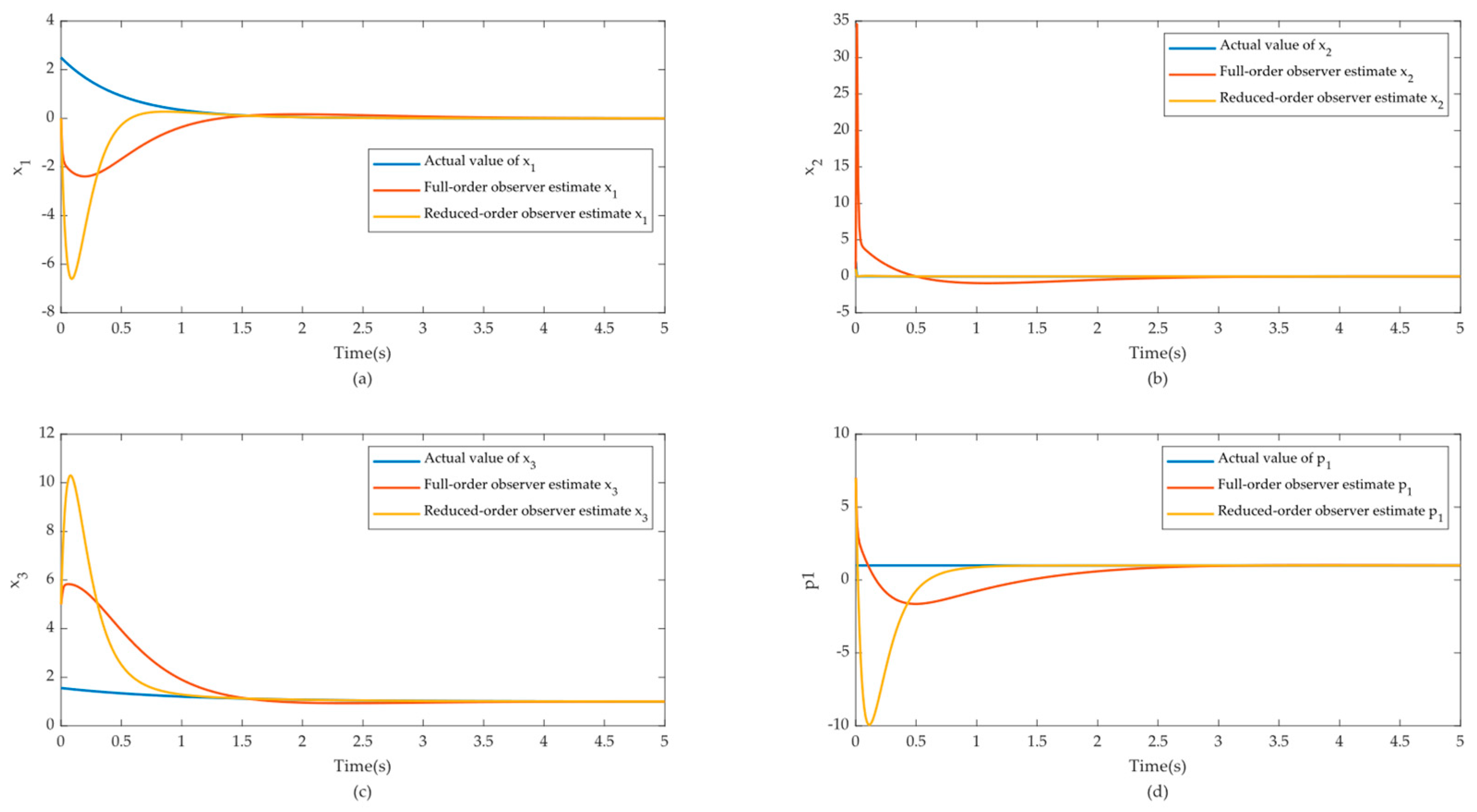
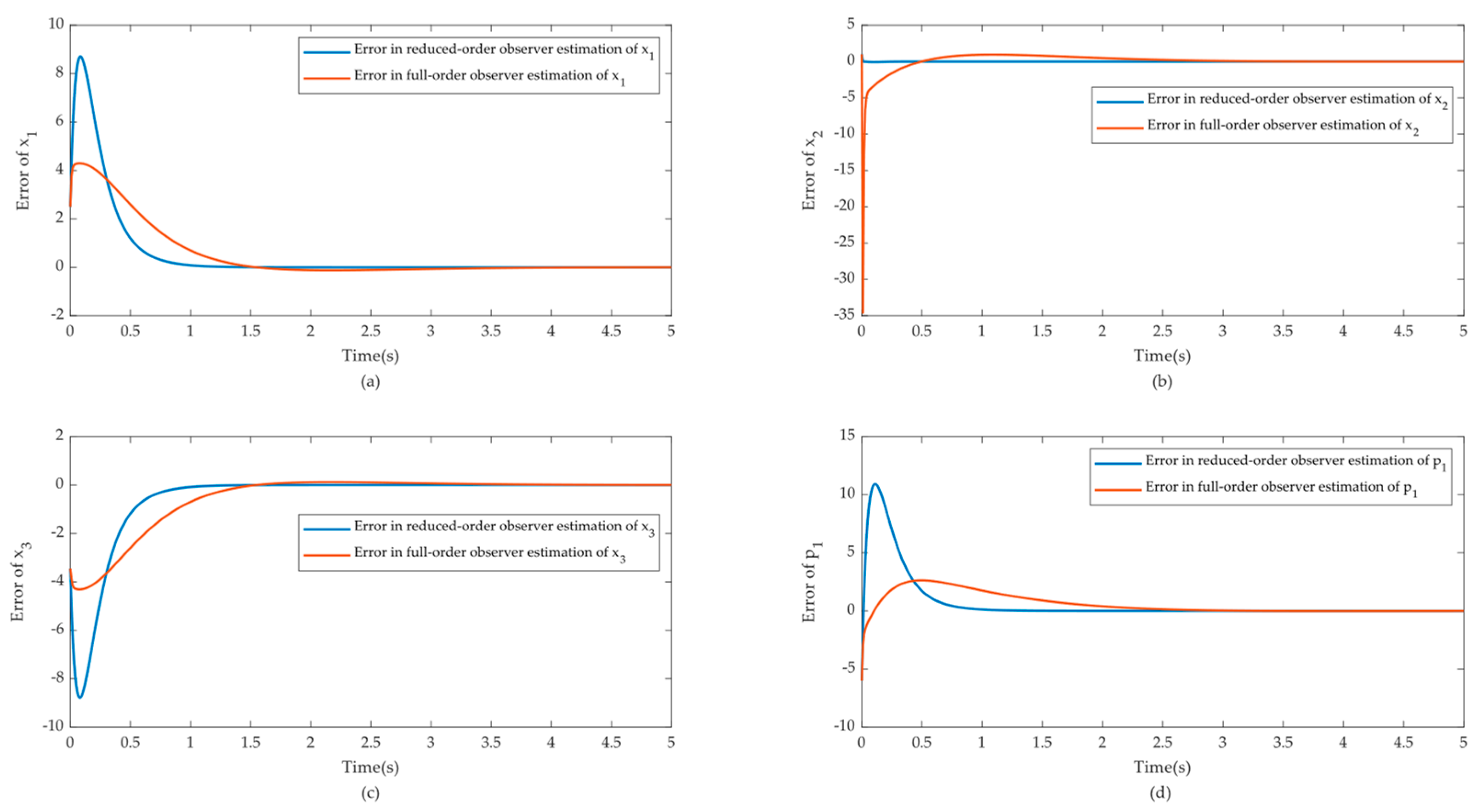
4.1. Numerical System

Consider the nonlinear numerical system:

$$\left\{\begin{array}{l}{\dot{x}}_1=-2x_1\hfill \\ {\dot{x}}_2=-1000x_2+p_1{x}_1\hfill \\ {\dot{x}}_3=x_2{x}_3-x_3+p_1\hfill \\ y=x_1+x_3\hfill \end{array}\right.$$

(21)

where $x_1$, $x_2$, $x_3$ are state variables and $p_1$ is system parameter.

The Lie derivative method [35] allows for the verification that the system is observable for all states and parameters. The steady state of the system is $\{0,0,p_1\}$ and its eigenvalues are $\{-2,-1000,-1\}$. It is observed that the system has two-time scales, and Assumptions 1–3 in Section 2 are satisfied after a suitable coordinate transformation. This section begins with the design of an observer for the original system (21) in order to illustrate the challenges of observer design for state and parameter estimation of nonlinear systems with two-time scales.

4.1.1. Observer Design Based on the Original System

Let the desired error dynamics eigenvalues be ${\lambda }_{\mathrm{f}}^{\mathrm{desired}}=-3000$, ${\lambda }_{\mathrm{s}}^{\mathrm{desired}}=\{-10,-5,-20\}$. As is common practice, the observer design parameter A can be selected arbitrarily, with the desired eigenvalues aligned on the diagonal. Similarly, the b matrix may be selected arbitrarily to ensure that the pair {A, b} is controllable.

Nevertheless, the design of an observer for this two-time-scale augmented system presents two significant challenges. Firstly, it is not straightforward to guarantee that the eigenvalues assigned to the observer align with the fast and slow modes of the system, thereby ensuring optimal performance of the error dynamics. In addition, the states and parameters estimation problem are more challenging due to the presence of calculation restrictions. The state-dependent observer gains are highly nonlinear, which make the solving process for the observer difficult to converge due to the stiffness. Therefore, the A and b matrices cannot be simply arbitrarily selected; they must be well designed. Following linearization and the implementation of a well-designed process [17], the matrices A and b are chosen as follows:

$$A=\left[\begin{array}{cccc}-653.48& 0& -651.48& 0\\ 967284.26& -1000& 967282.26& 0\\ -1380.52& 2& -1381.52& 1\\ -1500.00& 0& -1500.00& 0\end{array}\right],b=\left[\begin{array}{c}651.48\\ -967284.26\\ 1380.52\\ 1500.00\end{array}\right]$$

As can be observed from the matrix A, the elements are of disparate orders of magnitude, which causes the problem of ill-conditioning of the error dynamics and makes the calculation process more laborious. The full-order nonlinear observer (22) is calculated to provide an estimation of the state and parameters of the system (21).

$$\left[\begin{array}{c}{\widehat{x}}_1\\ {\widehat{x}}_2\\ {\widehat{x}}_3\\ {\widehat{p}}_1\end{array}\right]=\left[\begin{array}{c}-2{\widehat{x}}_1\\ -1000{\widehat{x}}_2+{\widehat{p}}_1{\widehat{x}}_1\\ {\widehat{x}}_2{\widehat{x}}_3-{\widehat{x}}_3+{\widehat{p}}_1\\ 0\end{array}\right]+L({\widehat{x}}_1,{\widehat{x}}_2,{\widehat{x}}_3,{\widehat{p}}_1)\left[(x_1+x_3)-({\widehat{x}}_1+{\widehat{x}}_3)\right]$$

(22)

Results are illustrated together with the outcomes of the following part in Figure 2 and Figure 3.

4.1.2. Observer Design Based on the Reduced-Order System

In order to address the challenges associated with the two-time-scale dynamics, the proposed observer design framework is employed. It is observed that the Jacobian matrix of the system (21) around the steady-state point is in upper triangular form. This implies that the diagonal elements of the matrix are exactly the eigenvalues of the system. Moreover, there is a direct correspondence between each state variable and the fast and slow eigenvalues, whereby $x_1$ and $x_3$ correspond to the slow system state and $x_2$ corresponds to the fast system state.

By defining $z=x_3-p_1$ and replacing $x_3$ with this new coordinate, the origin becomes the steady state, and the system is transformed to:

$$\left\{\begin{array}{l}{\dot{x}}_1=-2x_1\hfill \\ {\dot{x}}_2=-1000x_2+p_1{x}_1\hfill \\ \dot{z}=x_2(z+p_1)-z\hfill \\ y=x_1+z+p_1\hfill \end{array}\right.$$

(23)

In accordance with the proposed method, the fast dynamics can be projected onto the slow-motion invariant manifold, thereby reducing the original model to a lower-order model comprising only slow states. The slow-motion invariant manifold will be of the form $x_2=\pi (x_1,z)$, where $\pi (x_1,z)$ should satisfy the following invariance equation in the form of (7):

$$(-2x_1){\displaystyle \frac{\partial \pi (x_1,z)}{\partial x_1}}+(x_2(z+p_1)-z){\displaystyle \frac{\partial \pi (x_1,z)}{\partial z}}=-1000\pi (x_1,z)+p_1{x}_1$$

(24)

The series expansion method is employed for the solution of this PDE. By expanding the unknown variables in (24) around the origin and making the coefficients on both sides of the equation equal, the analytical solution of the slow invariant manifold of the system (23) is obtained as follows:

$$\pi (x_1)={\displaystyle \frac{1}{998}}{p}_1{x}_1$$

(25)

The third-order system is reduced to a second-order system through the application of the invariant manifold method. In order to distinguish the reduced-order system from the original system (21), the state and output are denoted as $\tilde{x}$ and $\tilde{y}$, respectively. With the original coordinate, the reduced-order system then takes the following form:

$$\left\{\begin{array}{l}{\dot{\tilde{x}}}_1=-2{\tilde{x}}_1\hfill \\ {\dot{\tilde{x}}}_3={\tilde{x}}_2{\tilde{x}}_3-{\tilde{x}}_3+p_1\hfill \\ {\tilde{x}}_2=\pi ({\tilde{x}}_1)={\displaystyle \frac{1}{998}}{p}_1{\tilde{x}}_1\hfill \\ \tilde{y}={\tilde{x}}_1+{\tilde{x}}_3\hfill \end{array}\right.$$

(26)

The augmented system for the observer design and parameter estimation is constructed as follows:

$$\left\{\begin{array}{l}{\dot{\tilde{x}}}_1=-2{\tilde{x}}_1\hfill \\ {\dot{\tilde{x}}}_3={\tilde{x}}_2{\tilde{x}}_3-{\tilde{x}}_3+p_1\hfill \\ {\dot{p}}_1=0\hfill \\ {\tilde{x}}_2={\displaystyle \frac{1}{998}}{p}_1{\tilde{x}}_1\hfill \\ \tilde{y}={\tilde{x}}_1+{\tilde{x}}_3\hfill \end{array}\right.$$

(27)

The next step is to design a full-order observer based on the augmented reduced-order system (27). In accordance with the preceding case, the desired eigenvalues of the observer are configured as ${\lambda }_{\mathrm{s}}^{\mathrm{desired}}=\{-10,-5,-20\}$. Given that only slow dynamics are present in the system, the matrices A and b can now be specified with greater ease:

$$A=\left[\begin{array}{ccc}-10& 0& 0\\ 0& -5& 0\\ 0& 0& -20\end{array}\right],b=\left[\begin{array}{c}1\\ 3\\ 2\end{array}\right]$$

The partial differential Equation (20) of $T({\tilde{x}}_{\mathrm{s}}^{\mathit{\vartheta }})=T({\tilde{x}}_1,{\tilde{x}}_3,p_1)$ is solved numerically using the truncated power series method in MATLAB, with an approximation obtained by retaining up to the third order term. Subsequently, the observer gain can be calculated as follows:

$$L({\tilde{x}}_1,{\tilde{x}}_3,p_1)={({\displaystyle \frac{\partial T({\tilde{x}}_{\mathrm{s}}^{\vartheta })}{\partial ({\tilde{x}}_{\mathrm{s}}^{\vartheta })}})}^{-1}b$$

(28)

In accordance with Formula (19), the observer derived from the reduced-order system (27) can be applied to the original system by substituting the actual output value $y$ from the system (21) in place of $\tilde{y}$. The observer for state and parameter estimation is thus obtained as follows:

$$\left\{\begin{array}{l}\left[\begin{array}{c}{\widehat{x}}_1\\ {\widehat{x}}_3\\ {\widehat{p}}_1\end{array}\right]=\left[\begin{array}{c}-2\cdot {\widehat{x}}_1\\ {\widehat{x}}_2\cdot {\widehat{x}}_3-{\widehat{x}}_3+{\widehat{p}}_1\\ 0\end{array}\right]+L({\widehat{x}}_1,{\widehat{x}}_3,{\widehat{p}}_1)\cdot \left[(x_1+x_3)-({\widehat{x}}_1+{\widehat{x}}_3)\right]\hfill \\ {\widehat{x}}_2={\displaystyle \frac{1}{998}}{\widehat{p}}_1{\widehat{x}}_1\hfill \end{array}\right.$$

(29)

Figure 2 and Figure 3 illustrate the actual and estimated values for states and parameters, and the estimation errors, respectively. The value of the parameter $p_1$ is fixed at 1. As illustrated in Figure 2 and Figure 3, both observers provide accurate estimation for states and parameters within a reasonable time frame. The estimation by the observer of the original system for fast state $x_2$ exhibits a notable overshoot and a slow convergence rate. In contrast, the reduced-order observer provides superior estimation for the fast state as the fast dynamics diminish almost instantaneously. The estimation of both states and parameters using reduced-order observers has yielded favorable results. This is due to the fact that, although the fast state is not taken into account when the reduced-order observer is designed, it is represented as an algebraic function of slow states using the slow-motion invariant manifold. Furthermore, the slow error dynamics can be accurately assigned to the slow mode of the system. Therefore, the missing of the fast dynamics does not have a notable impact on the estimation of parameters and states. It is noteworthy that by circumventing the stiffness issue associated with the two-time-scale system, the observer for the reduced-order system not only allows a more flexible selection of the A and b matrices during the design phase but also results in a more rapid calculation process for the observer system with enhanced convergence, effectively alleviating computational difficulties that would possibly be encountered in the two-time-scale system.

The numerical simulation illustrates the necessity of using the reduced-order observer for the parameter identification of the original system, as well as its favorable feasibility and accuracy. In this paper, the proposed reduced-order observer will be further applied and validated using an anaerobic digestion process as an example.

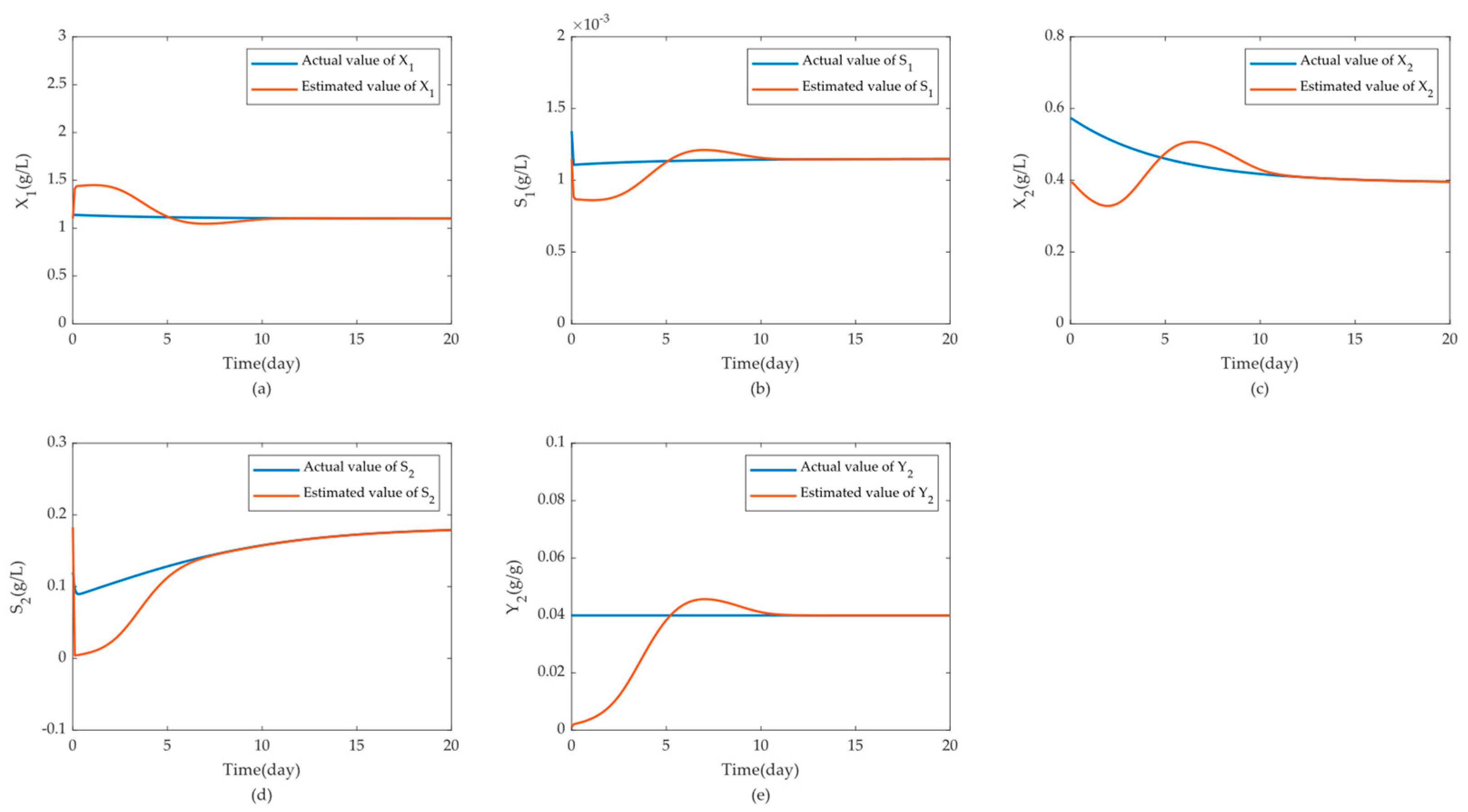
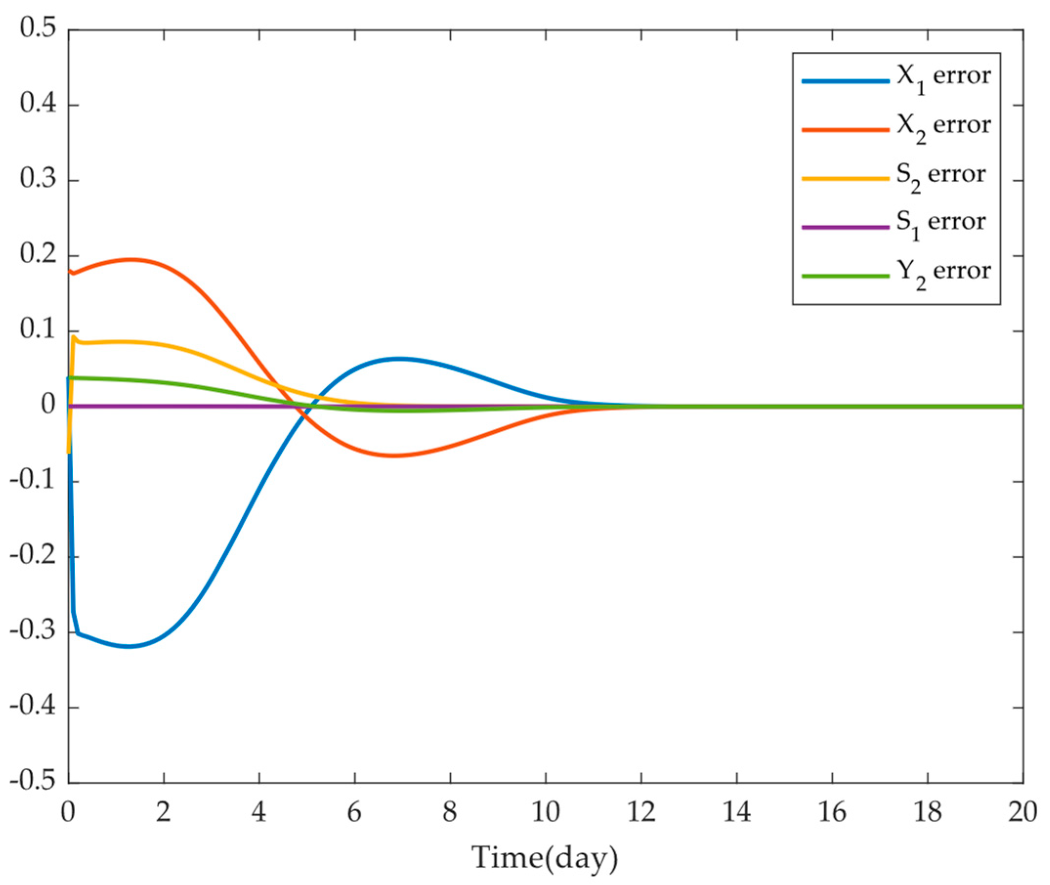
4.2. Anaerobic Digestion System

The anaerobic digestion process is a biological process whereby biogas is produced from biomass waste in the absence of oxygen. The system can be described as a typical multivariate, multi-stage, strongly coupled, and highly nonlinear complex system. Insoluble organic wastes cannot be utilized directly by oxygen- or methane-producing microorganisms, and the full anaerobic digestion process generally undergoes four stages: hydrolysis, acidogenesis, acetogenesis, and methanogenesis [39,40,41]. In this paper, for the sake of simplicity, a lumped model is employed to describe the anaerobic digestion as a two-step sequential process [33]. The first step, acidogenesis, contains faster-growing acidogenic bacteria, while the second step, methanogenesis, contains slower-growing methanogenic bacteria. Assuming that a continuously stirred bioreactor (CSTR) is used for the process and that only organic soluble substrates are present in the feed at a concentration of $S_1^0$, the aforementioned process can be expressed as follows:

$$\left\{\begin{array}{l}{\displaystyle \frac{d{X}_1}{dt}}=-D{X}_1+Y_1{\mu }_1(S_1)X_1\hfill \\ {\displaystyle \frac{d{S}_1}{dt}}=D(S_1^0-S_1)-{\mu }_1(S_1)X_1\hfill \\ {\displaystyle \frac{d{X}_2}{dt}}=-D{X}_2+Y_2{\mu }_2(S_2)X_2\hfill \\ {\displaystyle \frac{d{S}_2}{dt}}=-D{S}_2+c_2{\mu }_1(S_1)X_1-{\mu }_2(S_2)X_2\hfill \end{array}\right.$$

(30)

where $X_1$ is acidogenic bacteria, $S_1$ is organic soluble substrate, $S_2$ is a volatile fatty acid mixture, $X_2$ is the methanogenic bacterium. ${\mu }_1$ and ${\mu }_2$ are the specific consumption rates of $S_1$ and $S_2$ in the Monod and Haldane form as:

$$\left\{\begin{array}{l}{\mu }_1(S_1)={\displaystyle \frac{{\mu }_{\max 1}{S}_1}{Y_1(K_{\mathrm{s}1}+S_1)}}\hfill \\ {\mu }_2(S_2)={\displaystyle \frac{{\mu }_{\max 2}{S}_2}{Y_2(K_{\mathrm{s}2}+S_2+\frac{S_2^2}{K_{\mathrm{I}}})}}\hfill \end{array}\right.$$

(31)

The definition of all parameters and the reference values are shown in

Table 1. The definition of each parameter and the reference values of the model parameters [33].

Parameters	Implication	Value	Unit
$S_1^0$	Organic substrates concentration in feed	$10$	$\mathrm{g}/\mathrm{L}$
$D$	Dilution rate	$1.5$	${\mathrm{d}}^{-1}$
$Y_1$	Acid-producing bacteria yield coefficients	$0.11$	$\mathrm{g}/\mathrm{g}$
$Y_2$	Methanogenic bacteria yield coefficients	$0.04$	$\mathrm{g}/\mathrm{g}$
$c_2$	Stoichiometric coefficients for the conversion of organic substrates to volatile fatty acids	$1$	$\mathrm{g}/\mathrm{g}$
${\mu }_{\max 1}$	Maximum growth rate of acid-producing bacteria	$4.2$	${\mathrm{d}}^{-1}$
${\mu }_{\max 2}$	Maximum growth rate of methanogenic bacteria	$0.36$	${\mathrm{d}}^{-1}$
$K_{\mathrm{s}1}$	Saturation factor of acid producing bacteria	$0.023$	$\mathrm{g}/\mathrm{L}$
$K_{\mathrm{s}2}$	Saturation factor of methanogenic bacteria	$0.138$	$\mathrm{g}/\mathrm{L}$
$K_{\mathrm{I}}$	Inhibition factor of volatile fatty acids	$4$

:

The system exhibits four distinct steady states. The desired steady state under normal operating conditions with the given parameter values is $X_{1\mathrm{s}}=1.0999$, $S_{1\mathrm{s}}=0.0012$, $X_{2\mathrm{s}}=0.3926$ and $S_{2\mathrm{s}}=0.1830$. An analysis of the Jacobian matrix near this steady state reveals that the corresponding eigenvalues are ${\lambda }_1=-0.261$, ${\lambda }_2=-1656.12$, ${\lambda }_3=-0.261$ and ${\lambda }_4=-4.22$. It can be seen that ${\lambda }_2$ is much larger than the other eigenvalues, indicating that the system has two-time scales. It should be noted that ${\lambda }_2$ characterizes the speed of the chemical reaction involved in the acidogenesis step, which is typically much faster than both the dilution dynamics and the methanogenesis reactions represented by the other eigenvalues.

In practical applications, the concentrations of volatile fatty acids and total biomass can usually be measured, i.e., $y=[X_1+X_2\hspace{1em}{S}_2{]}^{\prime }$. In this case, the parameter methanogenic yield coefficient $Y_2$ is assumed to be unknown and thus requires estimation. It can be easily verified that the system is observable and that the parameter is identifiable with the output measurements.

In order to implement the proposed design framework, it is first necessary to conduct the model reduction to the system using the slow-motion invariant manifold method. This issue has been the subject of extensive investigation by Stamatelatou et al. [33].

In order to specify the fast and slow time scales of the system (30), a coordinate transformation is first performed. This involves replacing $X_1$ with a reaction invariant $Z=S_1-S_1^0+{\displaystyle \frac{X_1}{Y_1}}$ in the new coordinate system, which gives $X_1=Y_1(S_1^0-S_1+Z)$. Consequently, system (30) can be rewritten as follows:

$$\left\{\begin{array}{l}{\displaystyle \frac{dZ}{dt}}=-DZ\hfill \\ {\displaystyle \frac{d{S}_1}{dt}}=D(S_1^0-S_1)-{\mu }_1(S_1)Y_1(S_1^0-S_1+Z)\hfill \\ {\displaystyle \frac{d{X}_2}{dt}}=-D{X}_2+Y_2{\mu }_2(S_2)X_2\hfill \\ {\displaystyle \frac{d{S}_2}{dt}}=-D{S}_2+c_2{\mu }_1(S_1)Y_1(S_1^0-S_1+Z)-{\mu }_2(S_2)X_2\hfill \end{array}\right.$$

(32)

In this manner, the Jacobian matrix of the transformed system assumes a lower block triangular form, with $S_1$ representing the fast state characterized by the fastest eigenvalue ${\lambda }_2$. Under the assumption that the dynamics of the fast subsystem is instantaneous, the fast state $S_1$ is expressed as a function of the slow states using the slow invariant manifold, i.e., $S_1=\pi (Z)$, which can be solved according to the invariance condition (7).

$$(-DZ){\displaystyle \frac{d\pi (Z)}{dZ}}=D(S_1^0-\pi (Z))-{\displaystyle \frac{{\mu }_{\max 1}\pi (Z)}{K_{\mathrm{s}1}+\pi (Z)}}(S_1^0-\pi (Z)+Z)$$

(33)

The precise solution to Equation (33) is difficult to calculate, therefore an asymptotic solution is derived using a perturbation method with small quantities. With $\epsilon ={\displaystyle \frac{D}{{\mu }_{\max 1}}}\ll 1$ taken as the small parameter, the slow invariant manifold $\pi (Z)$ is obtained as follows:

$$\pi (Z)=K_{\mathrm{s}1}{\displaystyle \frac{S_1^0}{S_1^0+Z}}{\displaystyle \frac{D}{{\mu }_{\max 1}}}+K_{\mathrm{s}1}[{({\displaystyle \frac{S_1^0}{S_1^0+Z}})}^2-{\displaystyle \frac{2K_{\mathrm{s}1}{S}_1^{0}Z}{{(S_1^0+Z)}^3}}]{({\displaystyle \frac{D}{{\mu }_{\max 1}}})}^2+o({({\displaystyle \frac{D}{{\mu }_{\max 1}}})}^3)$$

(34)

Therefore, the fourth-order system is reduced to a third-order system through the application of the invariant manifold method, and the reduced order model of system (30) can be expressed as follows:

$$\left\{\begin{array}{l}{\displaystyle \frac{d\tilde{Z}}{dt}}=-D\tilde{Z}\hfill \\ {\displaystyle \frac{d{\tilde{X}}_2}{dt}}=-D{\tilde{X}}_2+Y_2{\mu }_2({\tilde{S}}_2){\tilde{X}}_2\hfill \\ {\displaystyle \frac{d{\tilde{S}}_2}{dt}}=D[c_2(S_1^0+Z{\displaystyle \frac{d\pi (Z)}{dt}}-\pi (Z))]-{\mu }_2({\tilde{S}}_2){\tilde{X}}_2\hfill \\ \begin{array}{l}{\tilde{S}}_1=\pi (\tilde{Z})\hfill \\ {\tilde{X}}_1=Y_1(S_1^0-\pi (\tilde{Z})+\tilde{Z})\hfill \\ \tilde{y}=[Y_1(S_1^0-\pi (\tilde{Z})+\tilde{Z})+{\tilde{X}}_2\hspace{1em}{\tilde{S}}_2{]}^{\prime }=\tilde{h}(\tilde{Z},{\tilde{X}}_2,{\tilde{S}}_2)\hfill \end{array}\hfill \end{array}\right.$$

(35)

The reduced order model (35) is used for the design of an observer for the estimation of states and the parameter methanogenic yield coefficient $Y_2$. Furthermore, the dynamics of a new state ${\displaystyle \frac{d{\tilde{Y}}_2}{dt}}=0$ are incorporated into the system (35) for augmentation, and the system used for observer design is as follows:

$$\left\{\begin{array}{l}{\displaystyle \frac{d\tilde{Z}}{dt}}=-D\tilde{Z}\hfill \\ {\displaystyle \frac{d{\tilde{X}}_2}{dt}}=-D{\tilde{X}}_2+Y_2{\mu }_2({\tilde{S}}_2){\tilde{X}}_2\hfill \\ \begin{array}{l}{\displaystyle \frac{d{\tilde{S}}_2}{dt}}=D[c_2(S_1^0+Z{\displaystyle \frac{d\pi (Z)}{dt}}-\pi (Z))]-{\mu }_2({\tilde{S}}_2){\tilde{X}}_2\\ {\displaystyle \frac{d{Y}_2}{dt}}=0\end{array}\hfill \\ \begin{array}{l}{\tilde{S}}_1=\pi (\tilde{Z})\hfill \\ {\tilde{X}}_1=Y_1(S_1^0-\pi (\tilde{Z})+\tilde{Z})\hfill \\ \tilde{y}=[Y_1(S_1^0-\pi (\tilde{Z})+\tilde{Z})+{\tilde{X}}_2\hspace{1em}{\tilde{S}}_2{]}^{\prime }=\tilde{h}(\tilde{Z},{\tilde{X}}_2,{\tilde{S}}_2)\hfill \end{array}\hfill \end{array}\right.$$

(36)

The desired error dynamics eigenvalues for the observer are set to ${\lambda }^{\mathrm{desired}}=\{-20,-5,-2,-13\}$, and the A and b matrices selected for use in this experiment are as follows:

$$A=\left[\begin{array}{cccc}-20& 0& 0& 0\\ 0& -5& 0& 0\\ 0& 0& -2& 0\\ 0& 0& 0& -13\end{array}\right],b=\left[\begin{array}{cc}10& 15\\ 5& 5\\ 5& 8\\ 3& 7\end{array}\right]$$

The system of PDEs in (20) is solved using the truncated power series method [42] in MATLAB up to truncation order 3. Subsequently, the state-dependent observer gain is calculated. The actual measured output value $y$ of the original system (30) is used in lieu of the output value $\tilde{y}$ of the reduced-order system to construct the reduced-order observer of the original system, which takes the following form:

$$\left[\begin{array}{c}\dot{\widehat{Z}}\\ {\dot{\widehat{X}}}_2\\ {\dot{\widehat{S}}}_2\\ {\dot{\widehat{Y}}}_2\end{array}\right]=\left[\begin{array}{c}-D\widehat{Z}\\ D{\widehat{X}}_2-{\widehat{Y}}_2{\mu }_2({\widehat{S}}_2,{\widehat{Y}}_2){\widehat{X}}_2\\ D[c_2(S_1^0+\widehat{Z}{\displaystyle \frac{d\pi (\widehat{Z})}{dt}}-\pi (\widehat{Z}))]-{\mu }_2({\widehat{S}}_2,{\widehat{Y}}_2){\widehat{X}}_2\\ 0\end{array}\right]+L(\widehat{Z},{\widehat{X}}_2,{\widehat{S}}_2,{\widehat{Y}}_2)\left(y-\widehat{y}\right)$$

(37)

The results of the observer estimations are presented in Figure 4, while the estimated errors are shown in Figure 5. As illustrated in Figure 4 and Figure 5, the observer developed based on the reduced-order model is shown to have the capacity to accurately estimate the states and parameters of the original system. In comparison to other states and parameters, the state $S_2$, which can be directly measured, demonstrates a faster convergence speed. With regard to the fast state $S_1$, which was disregarded during the design of the observer, the utilization of a reduced-order observer can promptly provide an accurate estimation and rapidly attain a stable state. Indeed, the direct design of observers for the original system presents significant challenges when considering the estimation of parameters in multi-time-scale nonlinear systems. While it is possible to configure observers for state and parameter estimation in some simple nonlinear systems after several attempts, as illustrated by the numerical case, the increasing stiffness, nonlinearity, and state-parameter coupling complexity in more complicated systems, like the anaerobic digestion process, make direct observer design markedly difficult. In contrast, the proposed framework allows for straightforward, feasible, and accurate parameter estimation of the original system. This effectively demonstrates the necessity and viability of the adopted observer design framework, which is capable of addressing the intricate challenges of complex two-time-scale nonlinear systems through a simplified approach.

5. Conclusions

This paper proposes an observer design framework for a class of two-time-scale nonlinear systems. The framework employs a reduced-order model, rendered using the slow-motion invariant manifold method, for the estimation of the states and parameters of the original system. The methodology proposed in this paper is validated through the convergence analysis of the error, as well as through the presentation of a numerical case study and an analysis of the anaerobic digestion process.

The numerical simulation and the simulation results of the anaerobic digestion system indicate that, since the reduced-order observer neglects the fast dynamics of the system, the issues of stiffness in the estimation of parameters for a multi-time scale nonlinear system, the complexity of designing an observer for such a system, and the computational burden associated with computing an observer for an ill-conditioned system can be alleviated. Furthermore, the proposed design approach provides preliminary estimates of the fast states based on a calculation rather than a random estimation, and also because the fast dynamics dissipate rapidly in a two-time-scale system, the exclusion of the fast dynamics does not result in a substantial impact, and the observer provides relatively precise estimations for the fast and slow states and parameters in both case studies.

References

1. Bernard, P.; Andrieu, V.; Astolfi, D. Observer design for continuous-time dynamical systems. Annu. Rev. Control 2022, 53, 224–248. [Google Scholar] [CrossRef]
2. Ding, F. Least squares parameter estimation and multi-innovation least squares methods for linear fitting problems from noisy data. J. Comput. Appl. Math. 2023, 426, 115107. [Google Scholar] [CrossRef]
3. Lathrop, P.M.; Duan, Z.; Ling, C.; Elabd, Y.A.; Kravaris, C. Modeling and observer-based monitoring of RAFT homopolymerization reactions. Processes 2019, 7, 768. [Google Scholar] [CrossRef]
4. Corigliano, A.; Mariani, S. Parameter identification in explicit structural dynamics: Performance of the extended Kalman filter. Comput. Methods Appl. Mech. Eng. 2004, 193, 3807–3835. [Google Scholar] [CrossRef]
5. Wang, C.; Wang, S.; Zhou, J.; Qiao, J.; Yang, X.; Xie, Y. A novel back propagation neural network-dual extended Kalman filter method for state-of-charge and state-of-health co-estimation of lithium-ion batteries based on limited memory least square algorithm. J. Energy Storage 2023, 59, 106563. [Google Scholar] [CrossRef]
6. Sheikholeslam, S. Observer-based parameter identifiers for nonlinear systems with parameter dependencies. IEEE Trans. Autom. Control 1995, 40, 382–387. [Google Scholar] [CrossRef]
7. Zhu, M.; Wen, Y.; Sun, W.; Lei, T. Extended state observer-based parameter identification of Nomoto model for autonomous vessels. Chin. J. Ship Res. 2023, 18, 75–85. [Google Scholar]
8. Patelski, R.; Pazderski, D. Novel adaptive extended state observer for dynamic parameter identification with asymptotic convergence. Energies 2022, 15, 3602. [Google Scholar] [CrossRef]
9. Marzougui, S.; Bedoui, S.; Atitallah, A.; Abderrahim, K. Parameter and state estimation of nonlinear fractional-order model using Luenberger observer. Circuits Syst. Signal Process. 2022, 41, 5366–5391. [Google Scholar] [CrossRef]
10. Cecilia, A.; Costa-Castello, R. Addressing the relative degree restriction in nonlinear adaptive observers: A high-gain observer approach. J. Frankl. Inst. 2022, 359, 3857–3882. [Google Scholar] [CrossRef]
11. Yildiz, R.; Demir, R.; Barut, M. Online estimations for electrical and mechanical parameters of the induction motor by extended Kalman filter. Trans. Inst. Meas. Control 2023, 45, 2725–2738. [Google Scholar] [CrossRef]
12. Yin, X.; Bo, S.; Liu, J.; Huang, B. Consensus-based approach for parameter and state estimation of agro-hydrological systems. AIChE J. 2021, 67, e17096. [Google Scholar] [CrossRef]
13. Backi, C.J.; Gravdahl, J.T.; Skogestad, S. Combined state and parameter estimation for not fully observable dynamic systems. IFAC J. Syst. Control 2020, 13, 100103. [Google Scholar] [CrossRef]
14. Afri, C.; Andrieu, V.; Bako, L.; Dufour, P. State and parameter estimation: A nonlinear Luenberger observer approach. IEEE Trans. Autom. Control 2016, 62, 973–980. [Google Scholar] [CrossRef]
15. Liu, J.; Gnanasekar, A.; Zhang, Y.; Bo, S.; Liu, J.; Hu, J.; Zou, T. Simultaneous state and parameter estimation: The role of sensitivity analysis. Ind. Eng. Chem. Res. 2021, 60, 2971–2982. [Google Scholar] [CrossRef]
16. Yin, X.; Liu, J. Distributed moving horizon state estimation of two-time-scale nonlinear systems. Automatica 2017, 79, 152–161. [Google Scholar] [CrossRef]
17. Duan, Z.; Kravaris, C. Nonlinear observer design for two-time-scale systems. AIChE J. 2020, 66, e16956. [Google Scholar] [CrossRef]
18. Yoo, H.; Gajic, Z. New designs of linear observers and observer-based controllers for singularly perturbed linear systems. IEEE Trans. Autom. Control 2018, 63, 3904–3911. [Google Scholar] [CrossRef]
19. Eilertsen, J.; Schnell, S.; Walcher, S. Rigorous estimates for the quasi-steady state approximation of the Michaelis–Menten reaction mechanism at low enzyme concentrations. Nonlinear Anal. Real World Appl. 2024, 78, 104088. [Google Scholar] [CrossRef]
20. Petrov, N.K. On the method of quasi-steady-state approximation. Mendeleev Commun. 2023, 33, 103–106. [Google Scholar] [CrossRef]
21. Patsatzis, D.G.; Goussis, D.A. Algorithmic criteria for the validity of quasi-steady state and partial equilibrium models: The Michaelis–Menten reaction mechanism. J. Math. Biol. 2023, 87, 27. [Google Scholar] [CrossRef]
22. Rao, S.; van der Schaft, A.; Jayawardhana, B. A graph-theoretical approach for the analysis and model reduction of complex-balanced chemical reaction networks. J. Math. Chem. 2013, 51, 2401–2422. [Google Scholar] [CrossRef]
23. Li, M.; Wang, R.Q.; Jia, G. Efficient dimension reduction and surrogate-based sensitivity analysis for expensive models with high-dimensional outputs. Reliab. Eng. Syst. Saf. 2020, 195, 106725. [Google Scholar] [CrossRef]
24. Hasan, B.M.S.; Abdulazeez, A.M. A review of principal component analysis algorithm for dimensionality reduction. J. Soft Comput. Data Min. 2021, 2, 20–30. [Google Scholar]
25. Tan, X.; Li, C.; Liu, D.; Wang, H.; Lu, X.; Zhu, Z.; Xu, R. Stability analysis and singular perturbation model reduction of DFIG-based variable-speed pumped storage unit adopting the fast speed control strategy. J. Energy Storage 2024, 87, 111340. [Google Scholar] [CrossRef]
26. Duan, Z.; Wilms, T.; Neubauer, P.; Kravaris, C.; Bournazou, M.N.C. Model reduction of aerobic bioprocess models for efficient simulation. Chem. Eng. Sci. 2020, 217, 115512. [Google Scholar] [CrossRef]
27. Mereles, A.; Alves, D.S.; Cavalca, K.L. Model reduction of rotor-foundation systems using the approximate invariant manifold method. Nonlinear Dyn. 2023, 111, 10743–10768. [Google Scholar] [CrossRef]
28. Jain, S.; Haller, G. How to compute invariant manifolds and their reduced dynamics in high-dimensional finite element models. Nonlinear Dyn. 2022, 107, 1417–1450. [Google Scholar] [CrossRef]
29. Hooshmand, H.; Fateh, M. Voltage control of flexible-joint robot manipulators using singular perturbation technique for model order reduction. J. Electr. Comput. Eng. Innov. 2022, 10, 123–142. [Google Scholar]
30. Farza, M.; Ménard, T.; Ltaief, A.; Maatoug, T.; M’Saad, M.; Koubaa, Y. Extended high gain observer design for state and parameter estimation. In Proceedings of the 2015 4th International Conference on Systems and Control (ICSC), Sousse, Tunisia, 28–30 April 2015; pp. 345–350. [Google Scholar]
31. Kazantzis, N.; Kravaris, C.; Syrou, L. A new model reduction method for nonlinear dynamical systems. Nonlinear Dyn. 2010, 59, 183–194. [Google Scholar] [CrossRef]
32. Brandon, J. Introduction to applied nonlinear dynamical systems and chaos. Math. Gaz. 1991, 75, 255. [Google Scholar] [CrossRef]
33. Stamatelatou, K.; Syrou, L.; Kravaris, C.; Lyberatos, G. An invariant manifold approach for CSTR model reduction in the presence of multi-step biochemical reaction schemes. Application to anaerobic digestion. Chem. Eng. J. 2009, 150, 462–475. [Google Scholar] [CrossRef]
34. Woodbury, D.P. Accounting for Parameter Uncertainty in Reduced-Order Static and Dynamic Systems; Texas A&M University: College Station, TX, USA, 2011. [Google Scholar]
35. Villaverde, A.F. Observability and structural identifiability of nonlinear biological systems. Complexity 2019, 2019, 8497093. [Google Scholar] [CrossRef]
36. Byrnes, C.I.; Pandian, S.V. Exponential observer design. In Nonlinear Control Systems Design 1992; Elsevier: Amsterdam, The Netherlands, 1993; pp. 215–218. [Google Scholar]
37. Kazantzis, N.; Kravaris, C. Nonlinear observer design using Lyapunov’s auxiliary theorem. Syst. Control Lett. 1998, 34, 241–247. [Google Scholar] [CrossRef]
38. Kravaris, C.; Hahn, J.; Chu, Y. Advances and selected recent developments in state and parameter estimation. Comput. Chem. Eng. 2013, 51, 111–123. [Google Scholar] [CrossRef]
39. Ram, N.R.; Nikhil, G.N. Assessment of microbial consortiums and their metabolic patterns during the bioconversion of food waste. Biomass Convers. Biorefinery 2023, 1–14. [Google Scholar] [CrossRef]
40. Nabaterega, R.; Kumar, V.; Khoei, S.; Eskicioglu, C. A review on two-stage anaerobic digestion options for optimizing municipal wastewater sludge treatment process. J. Environ. Chem. Eng. 2021, 9, 105502. [Google Scholar] [CrossRef]
41. Cárdenas, D.C.L.; Bournazou, M.N.C.; Barz, T.; Neubauer, P. Parameter Estimation, Ill-Conditioning and Identifiability Analysis of the Anaerobic Digestion Model No 1 (adm1) for Biogas Production. In Proceedings of the 2016 SIAM Annual Meeting, Boston, MA, USA, 11-15 July 2016. [Google Scholar]
42. Kazantzis, N. Singular PDEs and the problem of finding invariant manifolds for nonlinear dynamical systems. Phys. Lett. A 2000, 272, 257–263. [Google Scholar] [CrossRef]
Figure 1. Observer design methodology.
Processes 12 02875 g001
Figure 2. Dynamic response for actual and estimated states and parameter of the numerical system. (a) Actual and estimated values of x 1 ; (b) Actual and estimated values of x 2 ; (c) Actual and estimated values of x 3 ; (d) Actual and estimated values of p 1 .
Processes 12 02875 g002
Figure 3. Estimation errors for states and parameters of the numerical system. (a) Estimation error of x 1 ; (b) Estimation error of x 2 ; (c) Estimation error of x 3 ; (d) Estimation error of p 1 .
Processes 12 02875 g003
Figure 4. Comparison of original system values and estimated values for states and parameter (a) Actual and estimated values of X 1 ; (b) Actual and estimated values of S 1 ; (c) Actual and estimated values of X 2 ; (d) Actual and estimated values of S 2 ; (e) Actual and estimated values of Y 2 .
Processes 12 02875 g004
Figure 5. Observer estimation error of the anaerobic digestion system (the concentration of X 1 , X 2 , S 1 , S 2 are in g/L and the concentration of Y 2 is in g/g).
Processes 12 02875 g005