Investigation of a Cogeneration System Combining a Solid Oxide Fuel Cell and the Organic Rankine Cycle: Parametric Analysis and Multi-Objective Optimization

Abstract

A novel solid oxide fuel cell (SOFC)-based cogeneration system is proposed here, integrating an organic Rankine cycle for waste heat recovery. Technical–economic and parametric analyses are conducted, and a multi-objective optimization is carried out. The results reveal that the net electrical efficiency, investment cost, and payback time are 56.6%, USD 2,408,256, and 3.27 years, respectively. The parametric analysis indicates that the current density should be limited between 0.3 A/cm² and 0.9 A/cm², and the stack temperature should be controlled between 675 °C and 875 °C. After the operational optimization of η_ele-Cost_TCI, the investment cost and the net electrical efficiency are obtained as USD 2,164,742 and 62.1%. After the η_ele-PBT optimization, the payback period and the net electrical efficiency are 3.22 years and 58.9%. The heat transfer network optimization achieves the highest efficiency and reduces the cold utilities by 43 kW, but three additional heat exchangers should be added to the system. This research provides practical reference and pragmatic guidance for the integration, analysis, operation, and heat transfer network optimization of SOFC-based cogeneration systems.

1. Introduction

The depletion of fossil fuels and environmental pollution are becoming increasingly serious [1]. Against this background, it is particularly important to explore green energy generation contributing to sustainability and SDGs [2]. As a novel type of clean and efficient power generation equipment, fuel cells have received wide attention. With the maturity of technology and cost reduction, fuel cells can play a role in more areas [3,4].

Fuel cells can be categorized according to fuel type, electrolyte type, and operating temperature [5]. Among the many types of fuel cells, solid oxide fuel cells (SOFCs) are more adaptable to various fuels and are more efficient [6]. The high waste heat temperature of SOFCs can be effectively recovered through the establishment of a cogeneration system, further improving the efficiency of energy utilization [7]. The SOFC-based cogeneration system has become a very promising green energy-saving technology [8]. Many scholars have proposed novel SOFC-based cogeneration systems. Comprehensive performance evaluations and key parameter analyses of the systems have been carried out [9,10]. Zhu et al. [11] proposed a coupled system based on SOFCs, engine generation, and ARC. Parametric analyses showed that increasing the steam-to-biomass ratio or the fuel utilization contributed to an improvement in efficiency. Gholamian et al. [12] investigated SOFC-based hybrid systems coupled with either the organic Rankine cycle (ORC) or the Kalina cycle. It was found that the system coupled with the ORC had a higher energy efficiency of 62% than the energy efficiency of 60% of the system coupled with the KC cycle. Zeng et al. [13] designed waste-heat-driven hybrid systems with different configurations, using the ORC and absorption refrigeration cycle.

System optimization is a necessary step to further improve the operation performance of the proposed novel systems [14,15]. The combined processes need to be comprehensively evaluated from multiple aspects such as output, cost, and efficiency [16]. In most energy systems, the performance of the system is affected by multiple parameters, and it is difficult to achieve a trade-off between multiple objectives using a parametric analysis [17]. Therefore, many scholars often use algorithms to conduct multi-objective optimization. Wang et al. [18] used a genetic algorithm (NSGA-II) for the multi-objective optimization of a novel hybrid system. They indicated that the efficiency and the total cost rate of the atmospheric and pressurized systems reached 56.1% and 16.82 USD/h and 66.83% and 12.02 USD/h, respectively. Mahdi et al. [19] investigated a novel cogeneration system using the Gray Wolf optimization algorithm. The energy efficiency and exergy efficiency were obtained as 49.48% and 47.21%, respectively, in their objective optimization research. Abedinia et al. [20] conducted optimization research using a particle swarm approach coupled with an artificial neural network. Under optimal operating conditions, the highest exergy efficiency and the lowest total product cost were obtained as 42.71% and 6.29 USD/GJ. It can be seen that a lot of work has been carried out for the optimization of fuel-cell-based cogeneration systems, but the heat exchanger network is rarely considered in the system optimization.

Heat exchanger network optimization is one way to improve industrial energy efficiency [21]. Heat exchangers are the most common equipment in energy systems, especially cogeneration systems, which involve complex heat exchanger networks [22]. The optimization of heat exchanger network design is necessary to maximize energy efficiency and reduce costs [23]. Lei et al. [24] proposed an optimization model in which the HEN scheme was optimized with the operating parameters and working fluids at the same time. The HEN scheme was found to be an important reason for the different Pareto optimal solutions. Wang et al. [25] combined tri-reforming into an SOFC system and constructed four different heat transfer network configurations for the system. The results showed that configuration A, Reformer I-AOGR, gave the best performance. Huber et al. [26] optimized the coupling of a heat exchange network and operational parameters for a 1 MW hydroelectric unit. Zhang et al. [27] developed a multi-objective optimization method for the heat exchanger networks of a coal-to-methanol system, which reduced the power consumption by 29.6%.

The published literature mentioned above provides a solid foundation for fuel-cell-based systems, while fewer articles have investigated the interconnections among parameters and objectives after a thorough analysis of the system. In addition, the heat exchange network imposes an obvious impact on the system’s performance. However, the optimization of the heat exchange network is seldom considered with a parametric analysis at the same time. In this research, thermodynamic and economic analyses and a parametric analysis of the key parameters are conducted for a novel SOFC-based cogeneration system. Based on the analysis results of the proposed system, the heat exchange network is also considered for the operational optimization of this system. Then, the interconnections among the optimal parameters and objectives are investigated. The novel contributions can be concluded as the simultaneous optimization of the operational parameters and the heat transfer network of the system and the investigation of intrinsic connections among objectives and variables based on the parametric analysis. This work provides pragmatic information for the system integration, technical–economic and parametric analyses, operation, and heat transfer network optimization of SOFC-based energy utilization systems.

2. Methodology

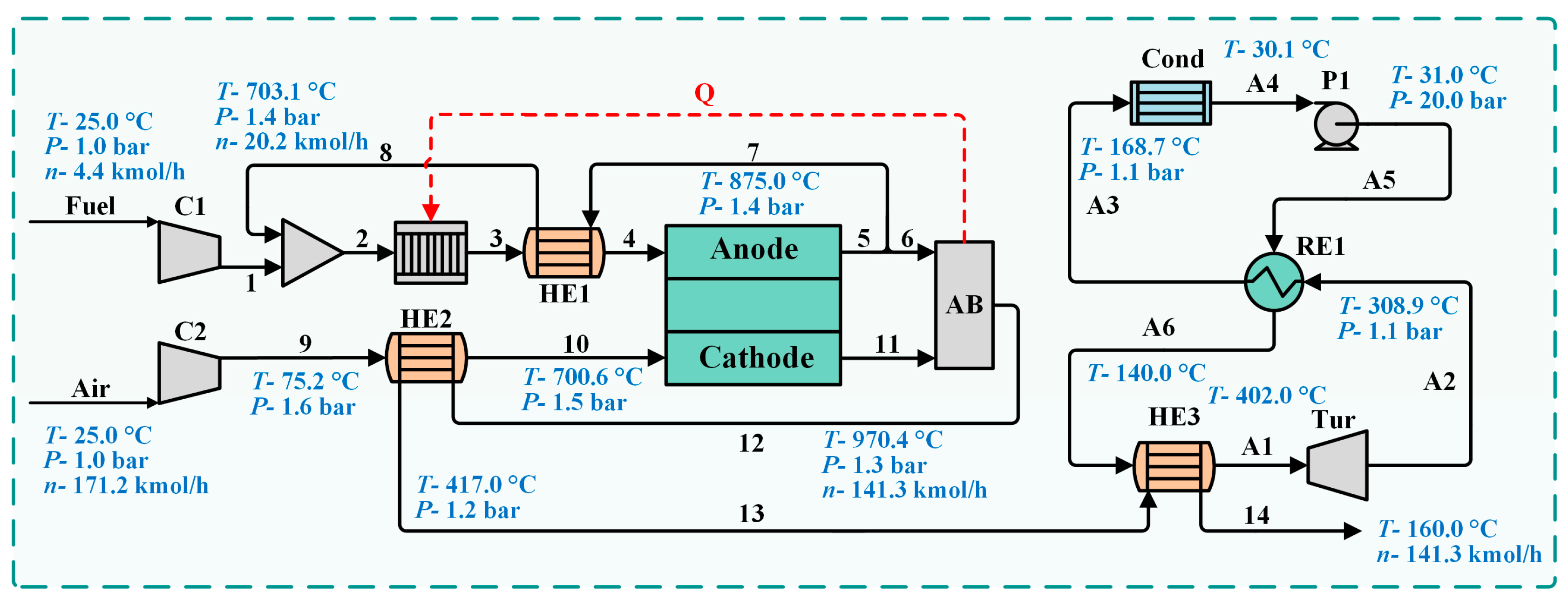
2.1. System Description

A flowchart of the SOFC-based cogeneration system is depicted in Figure 1, as a combination of an SOFC and the ORC. In the SOFC subsystem, the natural gas is pressurized and mixed with the anode recycle steam, and then it flows into the reformer for the reforming process. Pre-reforming can prevent carbon accumulation caused by improper operating conditions, which directly affects the performance and life of the stack. The SOFC stack has a certain tolerance to CO, so the obtained syngas (rich in hydrogen and carbon monoxide) directly enters the anode, and the air enters the cathode. In the stack, efficient electrochemical reactions generate electricity and heat. A part of the exhaust flows back to preheat the anode inlet syngas and then mixes with the fuel. Because the SOFC type is ionic conduction, the anode exhaust contains not only unreacted fuel but also water vapor, and the returned anode exhaust also provides the required water vapor needed for the reaction in the reformer. The other part of the anode exhaust and the cathode exhaust are burned in the burner. The heat released during combustion is fed to the reformer to maintain the heat required for the reforming reaction.

The high-temperature exhaust gases preheat the air and then drive the ORC subsystem. The temperature is still high after preheating the air. The ORC cycle is more suitable for higher heat source temperatures than the KC cycle. The heat source between 300 °C and 450 °C can drive the trans-critical cycle or the supercritical cycle. However, the heat source is a gas, which has a low heat capacity and a large temperature drop. And the operating pressure of trans-critical or supercritical cycles is high. Therefore, the ORC subsystem is used to recover waste heat from the system. In the ORC subsystem, the organic steam is first heated in a heat exchanger (HE5) by the waste heat from the SOFC subsystem. Then, these high-temperature and high-pressure vapors expand in the expander, converting thermal energy into electrical energy in the turbine. Finally, the organic steam is condensed into a liquid, and then it flows back to the heater exchanger. Thus, the SOFC and ORC subsystems provide electrical power to the load.

2.2. Simulation Models

(1)

Basic assumptions

The process simulation is conducted using the Aspen Plus software. The block specifications and descriptions are shown in

Table A1. Blocks used in establishing the systems.

Systems	Block type	Block ID	Description
SOFC subsystem	RGibbs	Ref	Simulate methane reforming process
	RGibbs	anode	Simulate the electrochemical reaction process
	Sep	cathode	Simulate oxygen ion transport
	RStoic	Burner	Simulate combustion reaction
	Compr	Comp1	Increase the pressure of the fuel
	Compr	Comp2	Increase the pressure of the air
	Heater	HE1	Preheated air
	Heater	HE2	Preheated air
	Mixer	Mix	Mix the stream
ORC subsystem	Compr	Tur	Convert the energy into mechanical work
	Heater	HE3	Heat recovery
	Heater	RE1	Heat the working fluid
	Heater	Cond1	Condense the working fluid
	Pump	P1	Increase the pressure of the working fluid

[28]. Peng-Rob is employed as the global physical property method [29]. The calculation of electrochemical models and multi-objective optimization are conducted in MATLAB 2019a. The basic assumptions are given as follows [30,31]: i. The chemical reaction is in equilibrium; ii. All gases are considered ideal; iii. The exhaust is completely consumed in the afterburner; iv. The pre-reformer and afterburner are adiabatic.

(2)

Pre-reformer reactor model

RGibbs is adopted for the CH₄ reforming, and the relevant reactions are given as Equations (1)–(3) [32]:

$$C{H}_4+H_{2}O\iff CO+3H_2$$

(1)

$$CO+H_{2}O\iff C{O}_2+H_2$$

(2)

$$C{H}_4+2H_{2}O\iff C{O}_2+4H_2$$

(3)

(3)

SOFC stack model

The residual CH₄ in the reformer is still useful in the stack because of the high temperature and catalyst in this stack, as in Equations (1)–(3). RGibbs and Splitter blocks are employed for the anode and cathode simulation, respectively [28]. Electrochemical reactions in the stack are given as follows. The process specifications of the stack are shown in

Table 1. Process parameters of SOFC [3,4,33].

Parameters	Value
Ncell	2054
Acell (cm2)	625
γa (A/m2)	7 × 109
γc (A/m2)	7 × 109
E0 (V)	E0 = 1.2723–2.7645 × 10−4 × T
ASRohm (Ωcm2)	0.04
Ean (J/mol)	110,000
Eca (J/mol)	160,000
Tair (°C)	25
Tfuel (°C)	25
Tatm (°C)	25
Patm (bar)	1
Uf/Ua	0.85/0.2
PSOFC (bar)	1.1

[33,34,35].

$$O_2+4e^{-}\to 2O^{2-}$$

(4)

$$H_2+O^{2-}\to H_{2}O+2e^{-}$$

(5)

$$CO+O^{2-}\to C{O}_2+2e^{-}$$

(6)

The stack power, current density, and voltage are calculated as follows [33,36,37]:

$$U_f={\displaystyle \frac{n_{H_{2,consumed}}}{n_{H_{2,equ}}}}$$

(7)

$$i={\displaystyle \frac{I}{A}}={\displaystyle \frac{2n_{H_{2,equ}}F{U}_f}{A}}$$

(8)

$$n_{H_{2,equ}}=n{H}_2+nCO+4nC{H}_4$$

(9)

$$W_{SOFC}=I·V$$

(10)

where i refers to the current density; A_cell refers to the stack active area; F refers to Faraday’s constant; and U_f refers to the fuel utilization factor.

$$V=V_N-V_{act}-V_{ohm}-V_{con}$$

(11)

$$V_N=E_0+{\displaystyle \frac{R{T}_{avg}}{4F}}\ln \left({\displaystyle \frac{P_{H_2}{P}_{O_2}}{P_{H_{2}O}{P}_{atm}^{0.5}}}\right)$$

(12)

where V represents the single-cell voltage; V_N refers to the Nernst voltage; E₀ = 1.2723–2.7645 × 10⁻⁴ × T; V_act refers to the activation loss; V_ohm is the ohmic loss; and V_con refers to the concentration loss. The activation loss (V_act) of the stack can be determined by the Butler–Volmer equation.

$$i=i_0[\exp (\alpha {\displaystyle \frac{nF}{RT}}{V}_{act})-\exp (-(1-\alpha ){\displaystyle \frac{nF}{RT}}{V}_{act})]$$

(13)

$$i_{0,c}={\gamma }_c{({\displaystyle \frac{P_{O_2}}{P_{atm}}})}^{0.25}\exp (-{\displaystyle \frac{E^{ca}}{RT}})$$

(14)

$$i_{0,a}={\gamma }_a({\displaystyle \frac{P_{H_2}}{P_{atm}}})({\displaystyle \frac{P_{H_{2}O}}{P_{atm}}})\exp (-{\displaystyle \frac{E^{an}}{RT}})$$

(15)

where i₀ is the pre-exponential factor that is specific to each electrode, γ is an activation overpotential factor, and E_act is the activation energy.

The ohmic loss (V_ohm) depends on the resistivity and thickness of the stacked elements. The stack ohmic loss can be approximated using the area-specific resistance by the following equation.

$$V_{ohm}=i·AS{R}_{ohm}$$

(16)

where ASR_ohm is the ohmic area-specific resistance estimated, 0.04 Ω cm².

Concentration loss (V_con) occurs mainly at high current densities, where the electrochemical reaction rate is fast and the reactants at the electrode are not replenished in a timely manner. It can be expressed by the following equation:

$$V_{con}={\displaystyle \frac{RT}{nF}}\ln (1-{\displaystyle \frac{i}{i_L}})$$

(17)

(4)

ORC subsystem

The corresponding models of ORC are provided in Table A1. The models follow the principle of energy and mass conservation [13]:

$$Q+{\displaystyle \sum m_{\mathrm{in}}{h}_{in}}=W_T+{\displaystyle \sum m_{out}}{h}_{out}$$

(18)

$${\displaystyle \sum m_{\mathrm{in}}}={\displaystyle \sum m_{out}}$$

(19)

2.3. Performance Indicators

(1)

Energy performance indicators

The stack net electrical efficiency η_SOFC:

$${\eta }_{SOFC}={\displaystyle \frac{W_{SOFC}-W_{Comp1}-W_{Comp2}}{m_{fuel}\cdot LH{V}_{fuel}}}\times 100\%$$

(20)

where W_comp1 and W_comp2 are the consumed electricity in Comp1 and Comp2 and LHV_fuel represents the lower heating value of the fuel.

The system net electrical efficiency η_ele is as follows:

$${\eta }_{ele}={\displaystyle \frac{W_{SOFC}+W_{Tur}-{\displaystyle \sum \left(W_{Comp}+W_P\right)}}{m_{fuel}\cdot LH{V}_{fuel}}}\times 100\%$$

(21)

(2)

Exergy performance indicators

Exergy refers to the qualitative value of energy, which includes the physical and chemical parts [38,39]:

$$Ex=E{x}^{ph}+E{x}^{ch}$$

(22)

$$E{x}^{ph}=m[h_{in}-h_{out}-T_0({\mathrm{s}}_{in}-s_{out})]$$

(23)

$$E{x}^{ch}={\displaystyle \sum _i^n{n}_i{\overline{ex}}_i^{ch,0}+R{T}_0{\displaystyle \sum _i^n{n}_i\ln x_i}}$$

(24)

(3)

Economic performance indicators

Economic indexes reveal the economic performance and clarify the investment and benefits of a project [40]. The total cost of this system (Cost_TCI) consists of two parts: the total depreciation cost (Cost_TDC) and startup cost (Cost_start). Among them, the total depreciation cost includes the fixed investment cost (Cost_fix), maintenance cost (Cost_maint), contingency cost (Cost_cont), and fuel cost (Cost_fuel) [41]. The cost equations are presented in

Table 2. Cogeneration system economic equations.

Cost	Equation
Fixed investment cost Costfix	Costfix
Maintenance cost Costmaint	Costmaint = 0.1 Costfix
Contingency cost Costcont	Costcont = 0.198 Costfix
Fuel cost Costfuel	Costfuel
Total depreciation cost CostTDC	CostTDC = Costfix + Costmaint + Costcont + Costfuel
Startup cost Coststart	Coststart = 0.1 CostTDC
Total cost of the system CostTCI	CostTCI = CostTDC + Coststart

.

The fixed investment cost is the cost of the system components (C_K). To estimate the system cost more accurately, this paper introduces the Chemical Engineering Plant Cost Index (CEPCI), which converts the calculated component costs for the year 2022 (CEPCI: 541.7) [42]. Detailed formulas for C_K and CEPCI_ref are shown in

Table A2. Component cost equations.

Components	Cost (USD)	Year	CEPCI
SOFC stack	$Z_{SOFC}=A_a{N}_{cell}(2.96T_{SOFC}-1907)$	2002	395.6
SOFC auxiliaries	$Z_{aux}=0.1\times Z_{SOFC}$	2002	395.6
SOFC inverter	$Z_{inv}={10}^5\times {(W_{SOFC}/500)}^{0.7}$	2002	395.6
Afterburner	$Z_{AB}={\displaystyle \frac{46.08m_6}{0.995-P_{in}/P_{out}}}(1+\exp (0.018T_{13}-26.4))$	1994	368.1
Compressor	$Z_{Comp}=91562{(W_{Comp}/445)}^{0.67}$	2003	402.3
Vale	$Z_{Vale}=114.5\times \dot{m}$	2001	394.3
Pump	$Z_P=705.48\times (1+0.2/(1-{\eta }_P))W_P^{0.71}$	2001	394.3
Turbine	$Z_{Tur}=W_{Tur}(1318.5-98.328\ln (W_{Tur}))$	2001	394.3
Preheater	$Z_{RE}=130\times {(A_{RE}/0.093)}^{0.78}$	2005	468.2
Heat exchanger	$Z_{HE}=130\times {(A_{HE}/0.093)}^{0.78}$	2000	394.1
Condenser	$Z_{Cond}=516.62\times A_{Cond}^{0.6}$	2005	468.2

[43].

$$C_{current}=C_{ref}\times {\displaystyle \frac{CEPC{I}_{current}}{CEPC{I}_{ref}}}$$

(25)

The fuel cost is obtained by using the following equation [44]:

$$C_{current}=C_{ref}\times {\displaystyle \frac{CEPC{I}_{current}}{CEPC{I}_{ref}}}$$

(26)

where c_f represents the natural gas unit cost of 3.5 USD/MMBTU.

Payback time (PBT) is a very important indicator in the economic evaluation of a project. PBT is the length of time it takes for a project to recover the full cost of investment from the start of the investment. PBT can be calculated by the following formula [45]:

$$PBT={\displaystyle \frac{\mathrm{Cos}{t}_{TDC}}{W_{net}{t}_w{C}_{elec}}}$$

(27)

where t_w represents the operating time of 7884 h, the system life is 15 years, W_net is the system net electrical output, and C_elec refers to the grid electricity price of 0.15 USD/kWh.

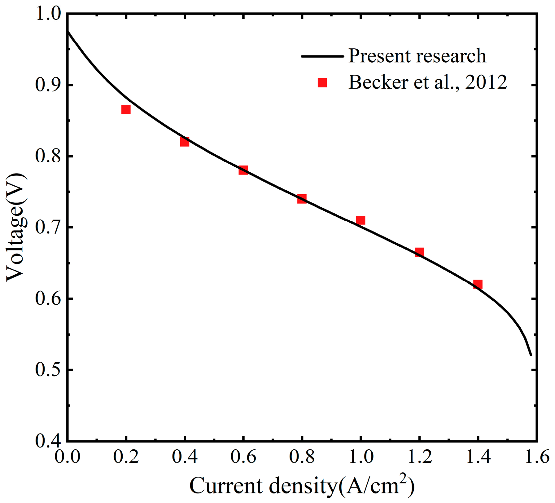
2.4. Model Verification

The modeling of the ORC subsystem is well-developed and does not involve complex physical processes. As the core component of a cogeneration system, the performance and reliability of the SOFC stack are critical to the effective operation of the entire system. Therefore, accurate stack modeling is key to the simulation of fuel cell cogeneration systems. During the SOFC stack model validation, it is common to compare the stack polarization curves obtained from the simulation with those from experimental data or other reliable references. Under the same parameter conditions (atmospheric pressure, operating temperature of 725 °C, and consistent feed), the polarization curves of the stack obtained in this research are compared with the polarization curves in reference [33], and the results are shown in Figure 2. As can be seen from the comparison, the error between the two is within 5%. This indicates that the established SOFC stack model has high reliability and accuracy.

3. Parametric and Performance Analyses

3.1. Current Density

The polarization curve in Figure 3a shows that the voltage of the SOFC decreases gradually as the current density increases. At a low current density, the voltage decreases faster, which is caused by the activation loss. And at high current density, the voltage drop tends to slow down, which is mainly caused by ohmic losses. Then, the stack power output improves with the rising current density. The change in current density is achieved by varying the fuel flow rates at a constant total polarization area. The improved system output is less than the fuel consumption, resulting in a decrease in efficiency.

In Figure 3b, the net efficiency of the SOFC stack goes down from 55% to 46%, and the system electrical efficiency goes down from 61% to 53.3% with the current density varying from 0.3 A/cm² to 0.9 A/cm². The total cost of the system increases linearly with increasing current density. As the current density rises to 0.4 A/cm², the PBT drops rapidly. At a current density from near 0.4 A/cm² to 0.9 A/cm², the PBT also decreases, but slower. With increasing current density at a low current density, the improvement in output power is more significant than the increase in total cost. As the current density increases, the increase in output power slows down. Therefore, the PBT decreases with increasing current density, but the trend is gradually smaller. The PBT increases even at current densities close to 0.9 A/cm². In summary, although the stack efficiency is as high as 60% at the current density of 0.1 A/cm², the electrical output is only 110 kW, and the PBT is high. This power is as high as 792 kW at the current density of 0.9 A/cm², but the efficiency of the stack drops to 46%, and the cost is high. Therefore, to ensure a proper stack operation, the current density should be limited in the range of 0.3 A/cm²–0.9 A/cm².

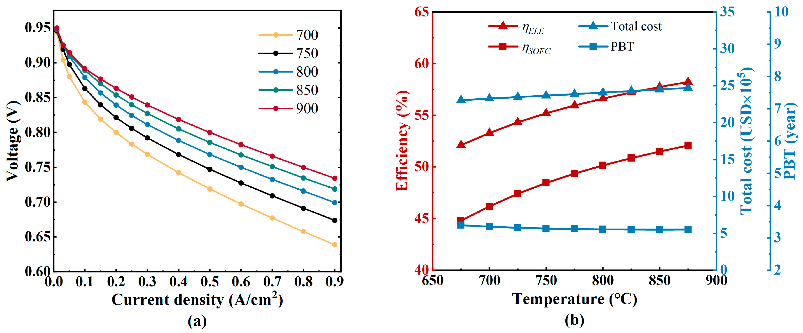
3.2. Average Stack Temperature

Figure 4a shows the polarization curves at different average stack temperatures. At a high current density, the effect of temperature on voltage is greater. The increase in temperature directly accelerates the rate of chemical reaction. At temperatures close to 900 °C, the water–gas reaction is limited, and the voltage increase will slow down. Figure 4b shows that the η_SOFC has increased but gradually slows down with the improving average temperature. The stack electrical output accounts for a major part of the system, so the trend of the η_ele is similar to the η_SOFC. As the average temperature increases from 675 °C to 950 °C, the η_SOFC increases from 45% to 52%, and the η_ele increases from 52% to 58%. The total cost increases as the average temperature increases but is not significant. The cost of each component and the output power both increase with the increase in temperature. Under the combined effect of the two, the PBT of the system is shortened from 3.40 years to 3.26 years, with the average temperature varying from 675 °C to 850 °C. However, the PBT is slightly increased when the average temperature improves from 850 °C to 875 °C. In conclusion, increasing the temperature of the stack will have a positive effect on the system. However, the increase is limited at high temperatures, and it will put higher demands on the materials of the components. Therefore, the average temperature of the stack should be moderate. The average temperature is taken to be between 675 °C and 875 °C in this paper.

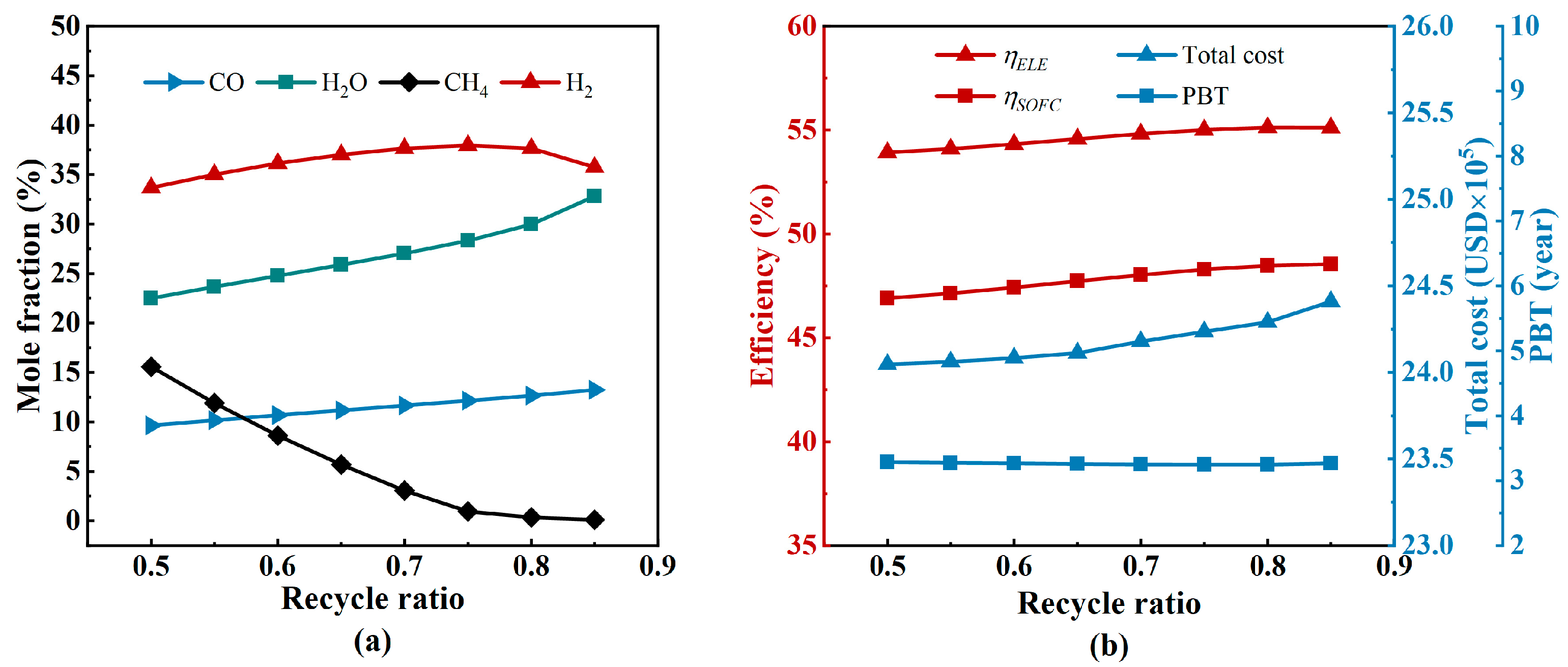
3.3. Anode Recycle Ratio

This parameter directly affects the reformer inlet temperature and water–carbon ratio. Figure 5a shows the variations in the reformer outlet composition for different recycle ratios. When the recycle ratio varies from 0.5 to 0.75, the mole fraction of methane drops rapidly, while the amount of H₂ and CO increases. If this ratio is further increased, the methane conversion is approaching the limit, and the residual water vapor gradually accumulates, resulting in a decrease in the mole fraction of H₂. The effect of the recycle ratio on the reforming conditions in the cogeneration system would influence the entire system. As shown in Figure 5b, the stack electrical efficiency and system electrical efficiency rise at first and then decrease as the recycle ratio increases from 0.5 to 0.85. The anode recycle ratio of the stack also affects the system economics, but the magnitude of the effect is small compared to the current density and stack temperature. The total cost consistently increases when increasing the recycle ratio, but the increase is less than 1 × 10⁵ USD; the system PBT decreases and then increases as the recycle ratio improves, but the change is less than 0.5 years. In summary, too small a recycle ratio increases the risk of carbon accumulation, and too large a recycle ratio leads to a decrease in the proportion of H₂, which results in lower efficiency, higher costs, and longer payback periods. Therefore, the recycle ratio of the cogeneration system in this paper should be in the range of 0.5 to 0.8.

3.4. System Performance

Based on the input parameters, the physical properties of each stream of this cogeneration system are obtained, as shown in

Table A3. Detailed stream data for SOFC subsystem.

Stream	Temperature (°C)	Pressure (bar)	Mole Flow (kmol/h)	Mole Fraction (%)
				N2	O2	CO2	CO	H2O	CH4	H2
Fuel	25.0	1.0	4.4	0	0	0	0	0	1	0
Air	25.0	1.0.	171.2	79.0	21.0	0.0	0	0	0	0
1	64.7	1.6	4.5	0	0	0	0	0	1	0
2	562.8	1.6	24.7	0	0	19.4	7.8	40.5	18.2	14.0
3	600.0	1.5	28.7	0	0	19.8	10.7	24.8	8.6	36.1
4	725.0	1.5	28.7	0	0	19.8	10.7	24.8	8.6	36.1
5	875.0	1.4	33.7	0	0	23.8	9.6	49.6	0	17.1
6	875.0	1.4	13.5	0	0	23.8	9.6	49.6	0	17.1
7	875.0	1.4	20.2	0	0	23.8	9.6	49.6	0	17.1
8	703.1	1.4	20.2	0	0	23.8	9.6	49.6	0	17.1
9	75.2	1.6	136.9	0.79	0.21	0	0	0	0	0
10	700.6	1.5	136.9	0.79	0.21	0	0	0	0	0
11	875.0	1.4	129.8	83.4	16.6	0	0	0	0	0
12	970.4	1.3	141.3	76.5	14.0	3.2	0	6.4	0	0
13	417.0	1.2	141.3	76.5	14.0	3.2	0	6.4	0	0
14	160.0	1.4	141.3	76.5	14.0	3.2	0	6.4	0	0

and

Table A4. Detailed stream data for ORC subsystem.

Stream	Temperature (°C)	Pressure (bar)	Mole Flow (kmol/h)	R123 Mole Fraction (%)
A1	402.0	20.0	20.86	100
A2	308.9	1.1	20.86	100
A3	168.7	1.1	20.86	100
A4	30.1	1.1	20.86	100
A5	31.0	20.0	20.86	100
A6	140.0	20.0	20.86	100

. The performance of the cogeneration system under the initial operating conditions is shown in

Table 3. Cogeneration system performance.

Parameters	Value	Parameters	Value
Current density i (A/m2)	6000	Single-cell voltage Vcell (V)	0.75
SOFC stack power WSOFC (kW)	566	Turbine power WTur (kW)	65
SOFC electrical efficiency ${\eta }_{SOFC}$ (%)	50.1	System electrical efficiency ηele (%)	56.6

and

Table 4. Cogeneration system economic equations.

Item	Value	Percentage
Fixed investment cost Costfix (USD)	593,377.5	24.6%
Maintenance cost Costmaint (USD)	59,337.75	2.5%
Contingency cost Costcont (USD)	117,488.7	4.9%
Fuel cost Costfuel (USD)	1,419,120	58.9%
Total depreciation cost CostTDC (USD)	2,189,324	90.9%
Startup cost Coststart (USD)	218,932.4	9.1%
Total cost of the system CostTCI (USD)	2,408,256	100%
Payback Time PBT (Year)	3.27	-

. In the cogeneration system, the SOFC stack output is 566 kW with a net stack efficiency of 50.1%, the turbine output is 65 kW, and the system total electrical power is 631 kW with a net electrical efficiency of 56.6%. The total investment in the cogeneration system amounted to USD 2,408,256, of which the total depreciation costs amounted to USD 2,189,324. The fuel cost is the main part of the total depreciation cost, which is 58.9%. The payback period is less than 4 years, indicating that the proposed system is profitable. Figure 6 illustrates the exergy destruction of each component. Significant exergy losses are found in the air preheater, afterburner, and the SOFC stack. The logarithmic mean temperature difference of the air preheater is calculated as higher than 300 °C. Hence, the huge exergy destruction occurs in this component because of its large load and heat transfer temperature difference. The afterburner burns the residual substances in the exhaust gas and converts the chemical energy of fuel into thermal energy, resulting in considerable exergy destruction because of the chemical reactions and substances mixing. Since the SOFC stack is the main fuel-consuming component in the system, it causes large exergy damage along with high energy consumption and output.

4. System Optimization

4.1. Optimization Model

For cogeneration systems, efficiency and cost are often important criteria for evaluating a system [46]. Both the total cost and PBT can describe the system’s economics. And in the system analysis, the total cost and the PBT will vary with the parameters. Therefore, the multi-objective optimization will make two cases: case 1, η_ele-Cost_TCI, and case 2, η_ele -PBT. To optimize the cogeneration system, the decision variables should be selected and specified [47]. Based on the system parameters and performance analysis, the current density, average stack temperature, and anode recycle ratio are selected as decision variables, as shown in

Table 5. Decision variables and ranges of values.

Decision Variables	Value Range	Unit
Current density	0.3–0.9	A/cm2
Average stack temperature	675–750	°C
Anode recycle ratio	0.5–0.8	-

.

Multiple heat exchangers are inevitably used in cogeneration systems, including air preheating, fuel preheating, and multiple waste heat recovery heat exchangers. The flow rates and temperatures vary greatly among the streams. Inefficient network configurations of heat exchange will lead to energy waste and cost increases. The heat exchanger network of a cogeneration system consists of cold streams (CS) and hot streams (HS), and then the heat exchanger network can be expressed as [24]:

$$Q_{HEN}={\displaystyle \sum _{i=1}^n{Q}_{HS,i}-Q_{CU}=}{\displaystyle \sum _{i=1}^n{Q}_{CS,i}-Q_{HU}}$$

(28)

$$Q_{HS,i}=c{p}_{HS,i}{m}_{HS,i}(T_{HS,i,in}-T_{HS,i,out})$$

(29)

$$Q_{CS,i}=c{p}_{CS,i}{m}_{CS,i}(T_{CS,i,in}-T_{CS,i,out})$$

(30)

Multi-objective optimization can deal with multiple objectives simultaneously and find the best trade-off solutions between these objectives, which can be achieved by genetic algorithms. A genetic algorithm is often utilized to achieve the optimal combination in terms of energy and exergy efficiencies, cost, and environmental performance. NSGA-II, with less computational complexity, is a common fast tool for solving multi-objective problems. The specifications for the genetic algorithm are listed in

Table 6. Genetic algorithm parameter values.

Algorithm Parameters	Values
Population size	100
Number of variables	3
Crossover ratio	80%
Proportion of variation	20%
Maximum number of iterations	100

.

Based on the model establishment described above, the genetic algorithm is employed for multi-objective optimization, and the flowchart of this algorithm is described in Figure 7. The Technique for Order Preference by Similarity to an Ideal Solution (TOPSIS) is an available decision-making method for final optimal solution selection [48]. It finds the optimal solution according to the relative proximities of each solution in the Pareto solution set computed by the distance from the positive ideal solution and the distance from the negative ideal solution. The final optimal solution is selected with the shortest distance from the ideal point and the farthest distance from the non-ideal point.

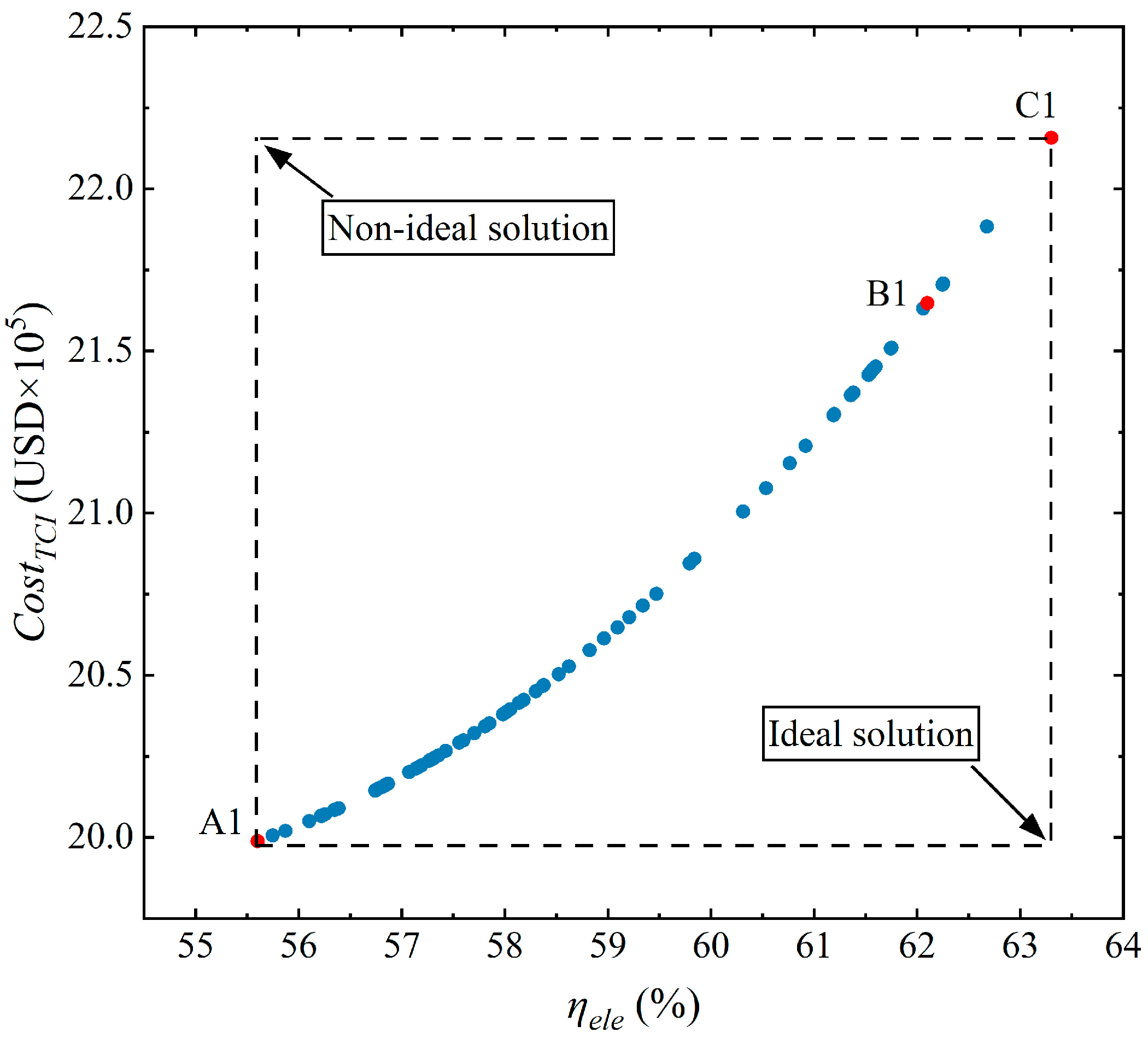
4.2. Optimization Results of Case 1 (ηele-CostTCI)

The Pareto frontier plot of case 1 (η_ele-Cost_TCI) is shown in Figure 8. A1 is the lowest point of total system cost, USD 1,998,885. But in this case, A1 has the lowest net electric efficiency of 55.6%. C1 is the highest point of net electric efficiency of the system at 63.3%, but simultaneously, it has the highest total cost of USD 2,215,737. B1 is the optimal point with a total cost of USD 2,164,742 and a net electrical efficiency of 62.1%.

The current density at A1, B1, and C1 is set to the lowest value. The reason for this is that as the current density increases, not only does the efficiency decrease, but also the total cost increases due to increased fuel consumption. Therefore, to achieve the goal of low cost and high efficiency, the current density chosen should be as low as possible. Secondly, the operating temperature of the stack at the three points increases sequentially. The operating temperature at point A1 is close to the minimum limit, while the operating temperature at point C1 is close to the maximum limit. The reason for this is that the system efficiency increases as the temperature rises, but accordingly, the cost of the system components increases. Therefore, a balance needs to be found between efficiency improvement and cost control. Finally, the anode recycle ratio at the three points is also gradually increased. However, unlike the operating temperature, the recycle ratio at point C1 does not reach the maximum limit. This is because when the recycle ratio is too high, it will reduce the system efficiency instead. The corresponding specifications are listed in

Table 7. Trade-off points for η_ele-PBT.

	Unit	A1	B1	C1
Current density	A/cm2	0.3	0.3	0.3
Stack temperature (average)	°C	677	843	875
Anode recycle ratio	-	0.51	0.60	0.78
ηele	%	55.6	62.1	63.3
CostTCI	USD	1,998,885	2,164,742	2,215,737
PBT	Year	3.58	3.57	3.67

.

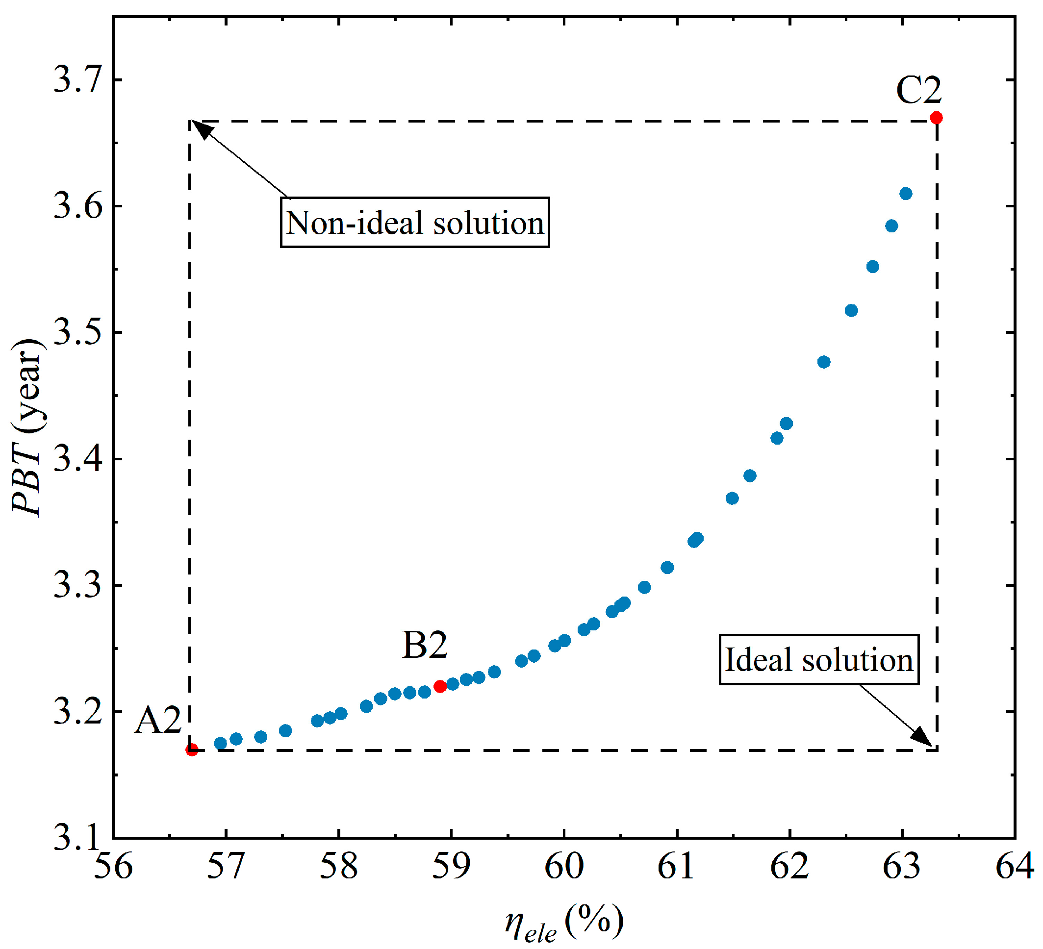
4.3. Optimization Results of Case2 (η_ele-PBT)

In the optimization results in case 1, although the three points of case 1 have high net electrical efficiency, the current density is only at the minimum limit, which leads to insufficient output power of the stack and a long PBT.

In Figure 9, the Pareto frontier plot of case 2 (η_ele-PBT) is shown, where A2 is the lowest point of the PBT at 3.17 years, but at this time, the lowest net electricity efficiency is 56.7%; C2 is the highest point of the system net electricity efficiency at 63.3%, but at this time, the PBT is the largest at 3.67 years; and B2 is the optimal point achieved by the entropy power method of trade-offs, with a recovery cycle of 3.22 and a net electricity efficiency of 58.9%. Points C1 and C2 both aim to achieve the highest net electrical efficiency, so they take the same values for the decision variables. At higher current densities, the output power of the system increases, which results in shorter payback periods. Therefore, in case 2, the current density settings at points A and B are higher than those in case 1. The increase in the operating temperature of the power stack will continue to increase the net power efficiency, but the recovery cycle will be shortened and then lengthened. Therefore, the SOFC stack temperatures of points A2 and B2 are set lower than C2. The corresponding specifications are given in

Table 8. Trade-off points for η_ele-PBT.

	Unit	A2	B2	C2
Current density	A/cm2	0.8	0.57	0.3
Stack temperature (average)	°C	850	850	875
Anode recycle ratio	-	0.65	0.62	0.78
ηele	%	56.7	58.9	63.3
PBT	Year	3.17	3.22	3.67
CostTCI	USD	3,136,668	2,363,673	2,215,737

.

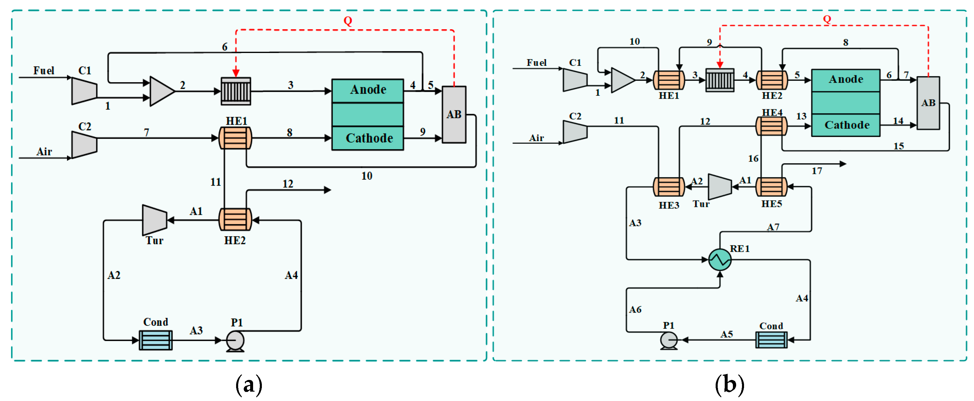
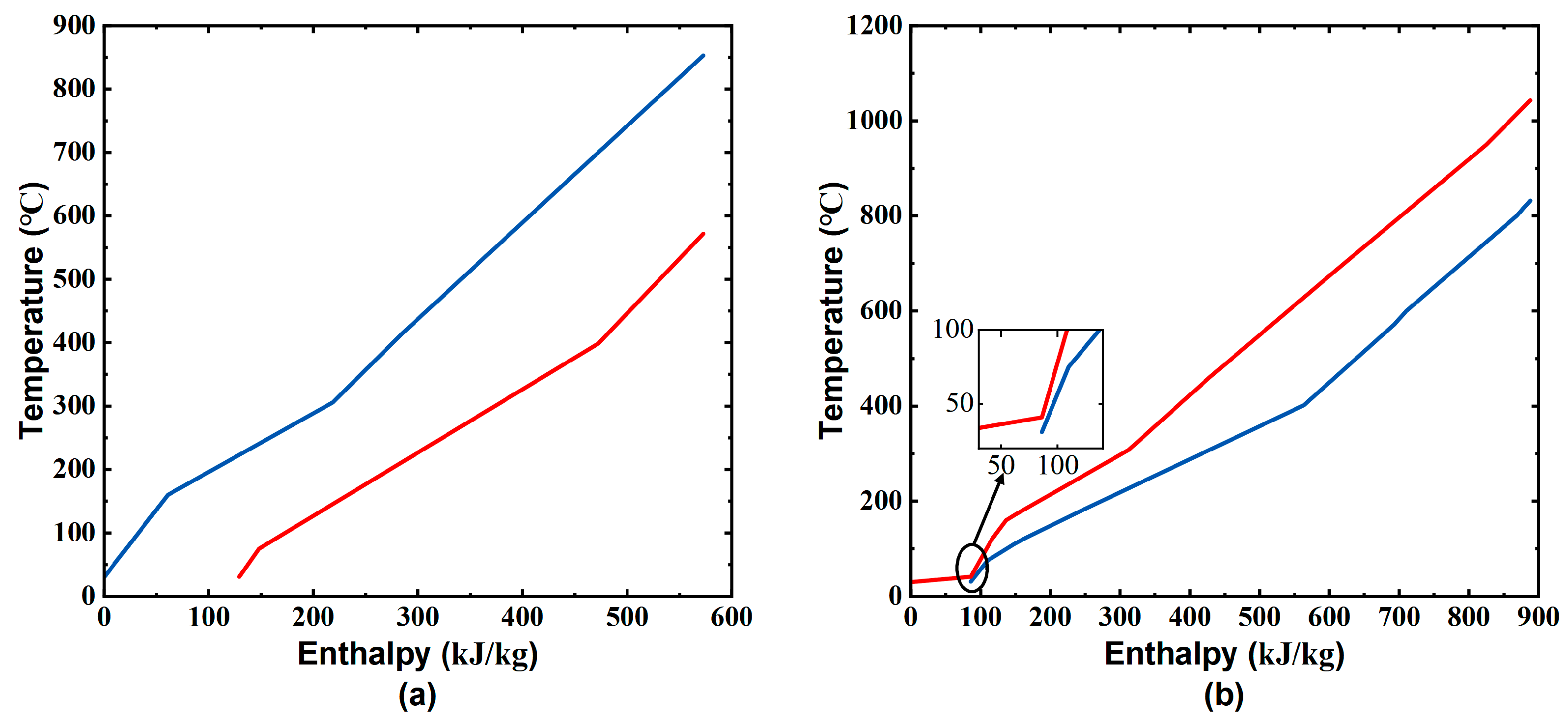
4.4. Optimization Results of Heat Exchange Network

The points in the Pareto frontier plot have different heat transfer network arrangements. Take point A1 as an example. As shown in Figure 10a, the heat exchanger network configuration at point A1 is extremely simplified, containing only two heat exchangers: the cathode preheater and waste heat recovery heat exchanger. This configuration ensures the basic operational requirements of the fuel cell system while minimizing the cost. Point C1 is then the most efficient configuration. As shown in Figure 10b, the heat transfer network at point C1 is more complex and contains five heat exchangers to improve system efficiency. The additional HE1 is used to avoid mixing the high-temperature anode recycle gas and the fresh fuel with large temperature differences and to reduce energy loss during mixing. By adding HE2 to achieve segmented preheated air, the temperature in the air preheater can be better matched and the turbine inlet temperature can be increased. Finally, RE1 was also added to the ORC cycle to recover the higher-temperature waste heat at the turbine outlet and reduce system energy loss. However, it is very practical that although the additional heat exchangers can improve the efficiency of this system, their addition inevitably increases the initial investment in equipment. Subsequently, auxiliary devices such as pipeline components will also be multiplied in the actual process. This puts forward higher requirements for the steady operation, sealing, and durability of the system.

The variation curves of the cold and hot flows of the heat transfer network corresponding to points A1 and C1 are shown in Figure 11. The minimum heat transfer temperature difference in the heat transfer network of A1 is large. The heat recovery of the system is 440 kW, and the cold utility consumption is 129 kW. The minimum heat transfer temperature difference in the heat transfer network of C1 is only 10 °C. The heat recovery of the system is 802 kW, and the cold utility consumption is 86 kW. In summary, the matching of the heat exchange temperature of the cogeneration system is achieved through the optimization of the heat exchanger network, thus improving the energy efficiency of the whole system. In the process of heat exchanger network optimization, additional heat exchangers are added to the system, and the layout of the existing heat exchangers is adjusted, which will lead to an increase in the initial investment cost.

5. Conclusions

This research achieves the simultaneous optimization of operational parameters and the heat transfer network of a novel SOFC-based cogeneration system and carried out an investigation of the intrinsic connections among the objectives and variables based on the parametric analysis results. A technical–economic analysis, a parametric analysis, and an operational and heat transfer network optimization were conducted. The main conclusions are summarized as follows:

(1)

The variations in current density and stack temperature lead to an imbalance between efficiency and economy. The current density is recommended to be between 0.3 A/cm² and 0.9 A/cm². The operating temperature of the SOFC stack should be limited between 675 °C and 875 °C. A lower recycle ratio would improve the risk of carbon accumulation, and a higher recycle ratio would reduce the efficiency and increase the total cost, so the recycle ratio of this system is recommended to be within 0.5–0.8.

(2)

Under initial conditions, the system net power efficiency, investment cost, and payback period are 56.6%, USD 2,408,256, and 3.27 years, respectively. In the case 1 (η_ele-Cost_TCI) optimization, the cost and the electrical efficiency of the optimal point are USD 2,164,742 and 62.1%. In the case 2 (η_ele-PBT) optimization, the PBT and the electrical efficiency of B2 are 3.22 years and 58.9%.

(3)

Comparing the two configurations of the heat exchange network for the lowest-cost purpose and highest-efficiency purpose, the former requires only two heat exchangers, while the latter requires five heat exchangers. The heat exchange network optimization reduces the consumption of cold utilities by 43 kW.

However, some limitations need to be clarified in this research: (1) only three operational parameters were selected for the decision variables; (2) the waste heat temperature would be different under different operating parameters, while the different cycles for waste heat recovery and the corresponding change in work quality were not investigated; (3) an uncertainty analysis is necessary as well, considering the variations and fluctuations of all the factors; (4) the impacts of operating environments (i.e., ambient temperature, atmospheric pressure, air composition, fuel composition, etc.) were not described in detail; (5) this research also neglects the requirements of the user. For future efforts, it is suggested that energy management strategies should be considered in the proposed system to achieve a fast and accurate response to the changing demands of the users.

References

1. Wang, L.; Guo, W.; Zhang, Z.; Wang, F.; Yuan, J. Performance analysis and optimization of syngas composition for reversible solid oxide fuel cells in dual-mode operation based on extreme learning machine. J. Power Sources 2024, 614, 234982. [Google Scholar] [CrossRef]
2. Vengatesan, S.; Jayakumar, A.; Sadasivuni, K.K. FCEV vs. BEV—A short overview on identifying the key contributors to af-fordable & clean energy (SDG-7). Energy Strategy Rev. 2024, 53, 101380. [Google Scholar] [CrossRef]
3. Song, M.; Zhuang, Y.; Zhang, L.; Li, W.; Du, J.; Shen, S. Thermodynamic performance assessment of SOFC-RC-KC system for multiple waste heat recovery. Energy Convers. Manag. 2021, 245, 114579. [Google Scholar] [CrossRef]
4. Song, M.; Zhuang, Y.; Zhang, L.; Wang, C.; Du, J.; Shen, S. Advanced exergy analysis for the solid oxide fuel cell system combined with a kinetic-based modeling pre-reformer. Energy Convers. Manag. 2021, 245, 114560. [Google Scholar] [CrossRef]
5. Zhao, J.; Cai, S.; Huang, X.; Luo, X.; Tu, Z. 4E analysis and multiobjective optimization of a PEMFC-based CCHP system with dehumidification. Energy Convers. Manag. 2021, 248, 114789. [Google Scholar] [CrossRef]
6. Tu, B.; Wen, H.; Yin, Y.; Zhang, F.; Su, X.; Cui, D.; Cheng, M. Thermodynamic analysis and experimental study of electrode reactions and open circuit voltages for methane-fuelled SOFC. Int. J. Hydrog. Energy 2020, 45, 34069–34079. [Google Scholar] [CrossRef]
7. Abbasi, H.R.; Pourrahmani, H.; Chitgar, N.; Van herle, J. Thermodynamic analysis of a tri-generation system using SOFC and HDH desalination unit. Int. J. Hydrog. Energy 2021, 72, 1204–1215. [Google Scholar] [CrossRef]
8. Singh, M.; Zappa, D.; Comini, E. Solid oxide fuel cell: Decade of progress, future perspectives and challenges. Int. J. Hydrog. Energy 2021, 46, 27643–27674. [Google Scholar] [CrossRef]
9. Ding, A.; Sun, H.; Zhang, S.; Dai, X.; Pan, Y.; Zhang, X.; Rahman, E.; Guo, J. Thermodynamic analysis and parameter optimization of a hybrid system based on SOFC and graphene-collector thermionic energy converter. Energy Convers. Manag. 2023, 291, 117327. [Google Scholar] [CrossRef]
10. Li, C.; Wang, Z.; Liu, H.; Guo, F.; Li, C.; Xiu, X.; Wang, C.; Qin, J.; Wei, L. Exergetic and exergoeconomic evaluation of an SOFC-Engine-ORC hybrid power generation system with methanol for ship application. Fuel 2024, 357, 129944. [Google Scholar] [CrossRef]
11. Zhu, P.; Wu, Z.; Guo, L.; Yao, J.; Dai, M.; Ren, J.; Kurko, S.; Yan, H.; Yang, F.; Zhang, Z. Achieving high-efficiency conversion and poly-generation of cooling, heating, and power based on biomass-fueled SOFC hybrid system: Performance assessment and multi-objective optimization. Energy Convers. Manag. 2021, 240, 114245. [Google Scholar] [CrossRef]
12. Gholamian, E.; Zare, V. A comparative thermodynamic investigation with environmental analysis of SOFC waste heat to power conversion employing Kalina and Organic Rankine Cycles. Energy Convers. Manag. 2016, 117, 150–161. [Google Scholar] [CrossRef]
13. Zeng, R.; Guo, B.; Zhang, X.; Li, H.; Zhang, G. Study on thermodynamic performance of SOFC-CCHP system integrating ORC and double-effect ARC. Energy Convers. Manag. 2021, 242, 114326. [Google Scholar] [CrossRef]
14. You, H.; Han, J.; Liu, Y.; Chen, C.; Ge, Y. 4E analysis and multi-objective optimization of a micro poly-generation system based on SOFC/MGT/MED and organic steam ejector refrigerator. Energy 2020, 206, 118122. [Google Scholar] [CrossRef]
15. Yuan, X.; Liu, Y.; Bucknall, R. Optimised MOPSO with the grey relationship analysis for the multi-criteria objective energy dispatch of a novel SOFC-solar hybrid CCHP residential system in the UK. Energy Convers. Manag. 2021, 243, 114406. [Google Scholar] [CrossRef]
16. Liang, W.; Yu, Z.; Liu, W.; Ji, S. Investigation of a novel near-zero emission poly-generation system based on biomass gasification and SOFC: A thermodynamic and exergoeconomic evaluation. Energy 2023, 282, 128822. [Google Scholar] [CrossRef]
17. Guo, Y.; Guo, X.; Wang, J.; Guan, Z.; Wang, Z.; Zhang, Y.; Wu, W.; Wang, X. Performance analysis and multi-objective optimization for a hybrid system based on solid oxide fuel cell and supercritical CO2 Brayton cycle with energetic and ecological objective approaches. Appl. Therm. Eng. 2023, 221, 119871. [Google Scholar] [CrossRef]
18. Wang, H.; Yu, Z.; Wang, D.; Li, G.; Xu, G. Energy, exergetic and economic analysis and multi-objective optimization of atmospheric and pressurized SOFC based trigeneration systems. Energy Convers. Manag. 2021, 239, 114183. [Google Scholar] [CrossRef]
19. Forootan, M.M.; Ahmadi, A. Machine learning-based optimization and 4E analysis of renewable-based polygeneration system by integration of GT-SRC-ORC-SOFC-PEME-MED-RO using multi-objective grey wolf optimization algorithm and neural networks. Renew. Sustain. Energy Rev. 2024, 200, 114616. [Google Scholar] [CrossRef]
20. Abedinia, O.; Shakibi, H.; Shokri, A.; Sobhani, B.; Sobhani, B.; Yari, M.; Bagheri, M. Optimization of a syngas-fueled SOFC-based multigeneration system: Enhanced performance with biomass and gasification agent selection. Renew. Sustain. Energy Rev. 2024, 199, 114460. [Google Scholar] [CrossRef]
21. Oliva, D.G.; Francesconi, J.A.; Mussati, M.C.; Aguirre, P.A. Ethanol and glycerin processor systems coupled to solid oxide fuel cells (SOFCs). Optimal operation and heat exchangers network synthesis. Int. J. Hydrog. Energy 2013, 38, 7140–7158. [Google Scholar] [CrossRef]
22. Fei, Z.; Yang, H.; Du, L.; Guerrero, J.M.; Meng, K.; Li, Z. Two-Stage Coordinated Operation of A Green Multi-Energy Ship Microgrid With Underwater Radiated Noise by Distributed Stochastic Approach. IEEE Trans. Smart Grid 2024, 1. [Google Scholar] [CrossRef]
23. Xu, Y.; Lei, Y.; Xu, C.; Chen, Y.; Tan, Q.; Ye, S.; Li, J.; Huang, W. Multi-objective optimization of a solid oxide fuel cell-based integrated system to select the optimal closed thermodynamic cycle and heat coupling scheme simultaneously. Int. J. Hydrog. Energy 2021, 46, 31828–31853. [Google Scholar] [CrossRef]
24. Lei, Y.; Ye, S.; Xu, Y.; Kong, C.; Xu, C.; Chen, Y.; Huang, W.; Xiao, H. Multi-objective optimization and algorithm improvement on thermal coupling of SOFC-GT-ORC integrated system. Comput. Chem. Eng. 2022, 164, 107903. [Google Scholar] [CrossRef]
25. Xuan Wang, R.H. Comparison and analysis of heat exchange and offgas recycle strategies in tri-reforming-SOFC system. Int. J. Hydrog. Energy 2023, 48, 34069–34079. [Google Scholar] [CrossRef]
26. Huber, D.; Birkelbach, F.; Hofmann, R. Unlocking the potential of synthetic fuel production: Coupled optimization of heat exchanger network and operating parameters of a 1 MW power-to-liquid plant. Chem. Eng. Sci. 2024, 284, 119506. [Google Scholar] [CrossRef]
27. Zhang, Z.; Zhao, L.; Tera, I.; Liu, G. Multi-objective optimization of heat exchanger network with disturbances based on graph theory and decoupling. Chem. Eng. Sci. 2024, 287, 119763. [Google Scholar] [CrossRef]
28. Doherty, W.; Reynolds, A.; Kennedy, D. Computer simulation of a biomass gasification-solid oxide fuel cell power system using Aspen Plus. Energy 2010, 35, 4545–4555. [Google Scholar] [CrossRef]
29. Anderson, T.; Vijay, P.; Tade, M.O. An adaptable steady state Aspen Hysys model for the methane fuelled solid oxide fuel cell. Chem. Eng. Res. Des. 2014, 92, 295–307. [Google Scholar] [CrossRef]
30. Wu, Z.; Tan, P.; Chen, B.; Cai, W.; Chen, M.; Xu, X.; Zhang, Z.; Ni, M. Dynamic modeling and operation strategy of an NG-fueled SOFC-WGS-TSA-PEMFC hybrid energy conversion system for fuel cell vehicle by using MATLAB/SIMULINK. Energy 2019, 175, 567–579. [Google Scholar] [CrossRef]
31. Alsarraf, J.; Alnaqi, A.A.; Al-Rashed, A.A.A.A. Thermodynamic modeling and exergy investigation of a hydrogen-based integrated system consisting of SOFC and CO2 capture option. Int. J. Hydrog. Energy 2022, 47, 26654–26664. [Google Scholar] [CrossRef]
32. Diglio, G.; Hanak, D.P.; Bareschino, P.; Pepe, F.; Montagnaro, F.; Manovic, V. Modelling of sorption-enhanced steam methane reforming in a fixed bed reactor network integrated with fuel cell. Appl. Energy 2018, 210, 1–15. [Google Scholar] [CrossRef]
33. Becker, W.L.; Braun, R.J.; Penev, M.; Melaina, M. Design and technoeconomic performance analysis of a 1MW solid oxide fuel cell polygeneration system for combined production of heat, hydrogen, and power. J. Power Sources 2012, 200, 34–44. [Google Scholar] [CrossRef]
34. Huang, Y.; Turan, A. Mechanical equilibrium operation integrated modelling of hybrid SOFC–GT systems: Design analyses and off-design optimization. Energy 2020, 208, 118334. [Google Scholar] [CrossRef]
35. Yang, S.; Jin, Z.; Ji, F.; Deng, C.; Liu, Z. Proposal and analysis of a combined cooling, heating, and power system with humidity control based on solid oxide fuel cell. Energy 2023, 284, 129233. [Google Scholar] [CrossRef]
36. Pirkandi, J.; Ghassemi, M.; Hamedi, M.H.; Mohammadi, R. Electrochemical and thermodynamic modeling of a CHP system using tubular solid oxide fuel cell (SOFC-CHP). J. Clean. Prod. 2012, 29–30, 151–162. [Google Scholar] [CrossRef]
37. Ma, L.; Ru, X.; Wang, J.; Lin, Z. System model and performance analysis of a solid oxide fuel cell system self-humidified with anode off-gas recycling. Int. J. Hydrog. Energy 2024, 57, 1164–1173. [Google Scholar] [CrossRef]
38. Sinha, A.A.; Saini, G.; Sanjay; Shukla, A.K.; Ansari, M.Z.; Dwivedi, G.; Choudhary, T. A novel comparison of energy-exergy, and sustainability analysis for biomass-fueled solid oxide fuel cell integrated gas turbine hybrid configuration. Energy Convers. Manag. 2023, 283, 116923. [Google Scholar] [CrossRef]
39. Wei, S.; Ni, S.; Ma, W.; Du, Z.; Lu, P. Exergy analysis and parameters optimization for zero-carbon/low-carbon fuels on SOFC-engine hybrid system. Fuel 2024, 364, 131076. [Google Scholar] [CrossRef]
40. Meng, N.; Li, T.; Jia, Y.; Qin, H.; Liu, Q.; Zhao, W.; Lei, G. Techno-economic performance comparison of enhanced geothermal system with typical cycle configurations for combined heating and power. Energy Convers. Manag. 2020, 205, 112409. [Google Scholar] [CrossRef]
41. Zhao, Z.; Shi, X.; Zhang, M.; Ouyang, T. Multi-scale assessment and multi-objective optimization of a novel solid oxide fuel cell hybrid power system fed by bio-syngas. J. Power Sources 2022, 524, 231047. [Google Scholar] [CrossRef]
42. Comidy, L.J.F.; Staples, M.D.; Barrett, S.R.H. Technical, economic, and environmental assessment of liquid fuel production on aircraft carriers. Appl. Energy 2019, 256, 113810. [Google Scholar] [CrossRef]
43. Su, Z.; Ouyang, T.; Chen, J.; Xu, P.; Tan, J.; Chen, N.; Huang, H. Green and efficient configuration of integrated waste heat and cold energy recovery for marine natural gas/diesel dual-fuel engine. Energy Convers. Manag. 2020, 209, 112650. [Google Scholar] [CrossRef]
44. Chitgar, N.; Emadi, M.A.; Chitsaz, A.; Rosen, M.A. Investigation of a novel multigeneration system driven by a SOFC for electricity and fresh water production. Energy Convers. Manag. 2019, 196, 296–310. [Google Scholar] [CrossRef]
45. Ouyang, T.; Zhao, Z.; Lu, J.; Su, Z.; Li, J.; Huang, H. Waste heat cascade utilisation of solid oxide fuel cell for marine applications. J. Clean. Prod. 2020, 275, 124133. [Google Scholar] [CrossRef]
46. Xia, W.; Ren, Z.; Li, H.; Pan, Z. A data-driven probabilistic evaluation method of hydrogen fuel cell vehicles hosting capacity for integrated hydrogen-electricity network. Appl. Energy 2024, 376, 123895. [Google Scholar] [CrossRef]
47. Yan, Z.; He, A.; Hara, S.; Shikazono, N. Modeling of solid oxide fuel cell (SOFC) electrodes from fabrication to operation: Microstructure optimization via artificial neural networks and multi-objective genetic algorithms. Energy Convers. Manag. 2019, 198, 111916. [Google Scholar] [CrossRef]
48. Xie, N.; Liu, Z.; Luo, Z.; Ren, J.; Deng, C.; Yang, S. Multi-objective optimization and life cycle assessment of an integrated system combining LiBr/H2O absorption chiller and Kalina cycle. Energy Convers. Manag. 2020, 225, 113448. [Google Scholar] [CrossRef]
Figure 1. Flowchart of the proposed system.
Processes 12 02873 g001
Figure 2. Verification of stack polarization curves [33].
Processes 12 02873 g002
Figure 3. Effect of current density on the system.
Processes 12 02873 g003
Figure 4. Effect of the average temperature of the stack on the system.
Processes 12 02873 g004
Figure 5. Effect of anode recycle ratio on the system.
Processes 12 02873 g005
Figure 6. Exergy destruction of each component.
Processes 12 02873 g006
Figure 7. Algorithm operation flowchart.
Processes 12 02873 g007
Figure 8. Pareto frontier plot for ηele-CostTCI.
Processes 12 02873 g008
Figure 9. Pareto frontier plot for ηele- PBT.
Processes 12 02873 g009
Figure 10. Flowchart corresponding to (a) A1 and (b) C1.
Processes 12 02873 g010
Figure 11. The combination curves of the cold and hot flow of (a) A1 and (b) C1.
Processes 12 02873 g011