Article

A Multi-Branch Deep Feature Fusion Network with SAE for Rare Earth Extraction Process Simulation

by
Fangping Xu
1,2,*,
Jianyong Zhu
1,2 and
Wei Wang
1,2
1
School Electrical and Automation Engineering, East China Jiaotong University, Nanchang 330013, China
2
State Key Laboratory of Performance Monitoring and Protecting of Rail Transit Infrastructure, East China Jiaotong University, Nanchang 330013, China
*
Author to whom correspondence should be addressed.
Processes 2024, 12(12), 2861; https://doi.org/10.3390/pr12122861
Submission received: 26 October 2024 / Revised: 7 December 2024 / Accepted: 11 December 2024 / Published: 13 December 2024
(This article belongs to the Section Process Control and Monitoring)

Abstract

:
The Rare Earth Extraction Process (REEP) model is difficult to accurately establish via the extraction mechanism method due to its high complexity. This paper proposes a multi-branch deep feature fusion network with SAE (SAE-MBDFFN) for modeling REEP. We first design a neural network with a multi-branch output structure to simulate the cascade REEP by introducing a multiscale feature fusion mechanism, which can simultaneously concatenate hidden features, original features, and inter-branch coupling features. In order to deal with insufficient labeled data during model training, we then adopt a stacked Sparse Auto-Encoder (SAE) technology to extract the hidden information of mass unlabeled data based on unsupervised learning. This technology can determine the initial parameters of SAE-MBDFFN by unsupervised pretraining. The design methodology of the network is well-founded. Experiments on industrial data indicate that the proposed method has the lowest initial loss value and a faster convergence rate in the fine-tuning stage than other comparison methods, while the prediction accuracy is better well. These results show the effectiveness of the proposed method.

1. Introduction

Rare Earth Elements (REEs), also known as industrial vitamins [1], have been widely used in various fields such as metallurgy, high-speed trains, and the national defense military industry [2]. The cascade extraction process, which is a cascade of many extraction tanks, is widely used to improve the purity of REs [3]. As a typical complex industrial process, the Rare Earth Extraction Process (REEP) is usually characterized by large nonlinear delays and strong coupling of various process variables [4]. However, adjusting the controlled parameters of the REEP often relies on manual experience, which can easily leads to poor performance and instability. Workers need to spend a great deal of time adjusting the parameters to stabilize the production status of the REE, especially when the feed conditions of production change; therefore, it is necessary to simulate the REEP in advance according to process data, as process simulation can quickly and accurately grasp the changes of component content (i.e., production index) to provide a decision basis for production [5]. At present, how to achieve process simulation for the REEP is an open problem.
Several scholars have used the extraction mechanism model to describe the REEP. In [6], an average fraction method based on the effective separation coefficient was proposed to calculate the component content of the REEP. In [7], a relative separation coefficient-based static calculation model was proposed to calculate the component content. Recently, Yun et al. [8] simplified the thermodynamic equilibrium equation to calculate the equilibrium concentration of REs in different extraction tanks. However, the extraction mechanism is unclear due to the complicated physicochemical reactions of REEP, which results in a mechanistic model with poor accuracy.
With the vigorous development of artificial intelligence and deep learning [9,10], scholars have begun to use data-driven methods to model the REEP. Giles et al. [11] used an artificial neural network to simulate the material transmission process for the REEP. The results showed their proposed method to be more accurate than the mechanism model. Backpropagation neural networks have also been applied to simulate the extraction equilibrium of RE solvents in order to predict the distribution ratio of rare earth elements between the organic phase and the aqueous phase [12]. In [13], Multiple Linear Regression (MLR), Stepwise Regression (SWR), and Artificial Neural Networks (ANNs) were used to simulate the REEP, fnding that the simulation results of the models were consistent with the actual values.
Nevertheless, it is well known that the performance of the neural networks depends on the completeness of labeled data [14], which need to be collected from the factory at substantial time and cost. To address insufficient label data, Zheng et al. [15] used a convolution stacked auto-encoder and t-distributed Stochastic Neighbor Embedding (t-SNE) algorithm to extract useful features from unlabeled data. In [16], a semi-supervised training strategy with auto-encoder was proposed to automatically adjust the training process according to whether or not the input data are labeled, which makes the model learn the hidden information of the unlabeled data. Further, in [17], a Semi-Supervised Deep Sparse Auto-Encoder (SSDSAE) with both local and nonlocal information was proposed to increase the robustness of the network for intelligent fault diagnosis of rotating machinery. From the above, it can be concluded that auto-encoder networks represent an effective solution for cases of insufficient labeled industrial data.
In addition, existing methods have only designed simple shallow models to obtain the component content of the extraction tank. However, in process simulation of the REEP it is necessary to obtain the component content of every extraction tank [18]. Due to the limitation of having only a single hidden layer structure, shallow neural networks cannot meet this accuracy requirement, as such methods cannot accurately describe a REEP with many extraction tanks. For example, solutions based on LS-SVM [19] or Neural Networks (NNs) [12] are only able to display the prediction results in the final output layer. Thus, shallow models do not consider the extraction tank in the posterior sequence of REEP, the deep models can easily lead to NNs overfitting the component content of the more forward extraction tanks. Hence, it is necessary to set up many NNs with different hidden layers to obtain the component content of all extraction tanks. However, these independent neural networks cannot consider the cascade relationship between extraction tanks and computing resources. In order to solve these problems, in the current paper we innovatively propose a Multi-Branch Deep Neural Network (MBDNN). In this neural network architecture, side branches are added to the main branch, allowing the component content of the forward extraction tanks to be output earlier than in the original baseline neural network. In this way, the network outputs the component content of the cascade extraction tanks through the branch layer, which meets the process simulation requirements for the REEP.
At present, the research on MBDNNs has mainly focused on classification problems. In [20], BranchyNet added side (lateral) branch classifiers to the traditional CNN structure, allowing image prediction results with different confidence to be output from different branches to reduce computational redundancy. Multi-Branch Neural Network (MB-Net) [21] was proposed to solve manual annotation of different remote sensing image datasets. This approach successfully boosted the average accuracy over all transfer scenarios to 89.05%, representing an improvement over standard architectures. In [22], Chen et al. designed an end-to-end trainable two-branch Partition and Reunion Network (PRN) for the vehicle re-identification task. Through structural innovations, multi-branch networks have achieved good results in image classification and fault diagnosis [23,24,25]. However, to the best of our knowledge, this kind of MBDNN has rarely been discussed for multiple-output regression problems [26] in complex industrial processes.
In this paper, we propose the Multi-Branch Deep Feature Fusion Network with Sparse Auto-Encoder for REEP modeling, which we call SAE-MBDFFN. We first design a multi-branch deep neural network with multiple outlets to obtain the multi-stage component content of the REEP. For SAE-MBDFFN, a multiscale feature fusion mechanism is introduced to overcome gradient disappearance. Due to the limited amount of labeled data and large amount of unlabeled data in the REEP, an unsupervised pretraining method based on stacked sparse auto-encoder is proposed to determine initial value of the hidden layer. Compared with random initialization of the parameters, the proposed unsupervised pretraining method leads to faster objective function convergence. In summary, the specific innovations of this paper are as follows:
(1)
We propose a Multi-Branch Deep Feature Fusion Network (MBDFFN) to build a simulation model for the cascaded REEP. To overcome gradient disappearance, we introduce multiscale feature fusion in the branch layer via the residual attention structure and the branch feature short connection.
(2)
Second, we present a stacked SAE-based unsupervised pretraining method for MBDFFN to determine the initial parameters of the network. Supervised fine-tuning on SAE-MBDFFN is then utilized to obtain the simulation model of the REEP.
(3)
Finally, simulation results show that our proposed SAE-MBDFFN achieves better performance compared to conventional neural networks and models that do not utilize pretraining.
In summary, this paper proposes a method for simulating the Rare Earth Extraction Process (REEP) by combining prior information extraction and a multi-branch neural network. Simulation results show that the proposed method has a small error for component content prediction and is able to meet actual production needs, which can provide intelligent decision support for process reorganization and parameter optimization.
The rest of this article is structured as follows: in Section 2, the principles of REEP and sparse auto-encoder algorithms are briefly introduced; then, the proposed multi-branch deep feature fusion network combined with SAE is described in detail in Section 3, which also introduces the unsupervised fine-tuning training process and REEP modeling steps; subsequently, the proposed method is verified using an the RE extraction factory dataset in Section 4; finally, Section 5 summarizes the main contributions of this article.

2. Introduction to the Rare Earth Extraction Process (REEP) and Sparse Auto Encoders

2.1. Description of the REEP

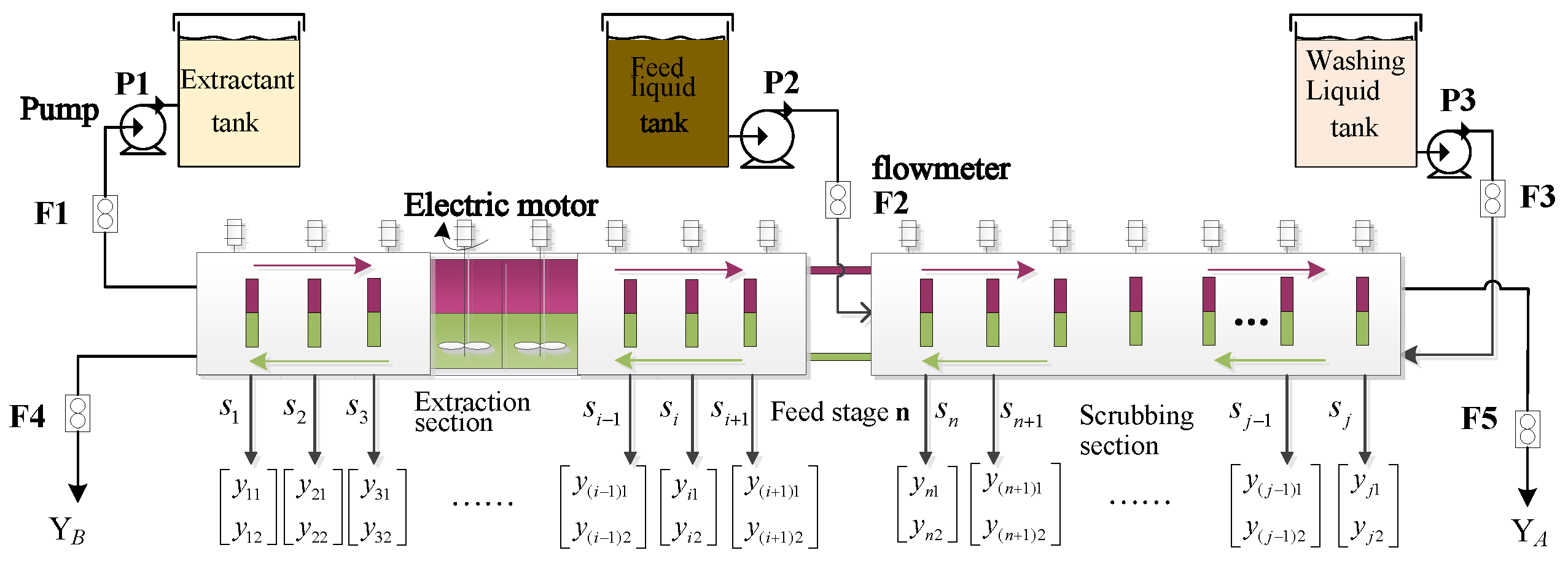
Because the separation factor between rare earth elements (REEs) is small, it is difficult to obtain the ideal component content of REEs using only a single extraction tank. Therefore, factories usually cascade a certain number of extraction tanks to ensure that REE liquids are continuously mixed, stirred, separated, and clarified under the action of the detergent and extractant [18]. Figure 1 depicts the production flow of the REEP, which involves the stages of extraction and scrubbing. Here, j = n + m, where each stage contains the corresponding mixer–settler number.
In REEP, the detergent and extractant are injected in the first and last stages respectively, with the liquid raw material is added between these stages. Then, the rare earth liquid appears with up-and-down stratification during the clarification process. Generally, the elements in the upper solution are called easy-to-extract components (i.e., organic phase), while the elements in the lower solution are called difficult-to-extract components (i.e., aqueous phase). The upper organic-phase liquid flows from left to right, while the lower aqueous phase solution has the opposite direction. After this process, the aqueous phase product with content Y B can be obtained from the first extraction tank, while the organic phase product with content Y A can be obtained at the last stage. For the i-th extraction tank, the corresponding component content value is Y i = [ y i 1 , y i 2 ] , i [ 1 , n + m ] , where y i 1 indicates the component content of the organic phase elements and y i 2 indicates component content of the aqueous phase elements.
Obviously, when the raw rare earth solution changes, the product quality (component content) changes during the REEP as well; therefore, obtaining these changes in a timely and accurate fashion is an important prerequisite for quickly adjusting the controlled parameters during production. Process simulation of the REEP is considered to be an effective method, as it can avoid the need for workers to spend time and cost on stabilizing the production status of the REEP when the raw REE solution changes.
In the REEP, the a relationship between the component content and the feed parameters is Y = g ( X , T ) , where Y = [ y i 1 , y i 2 ] represent the component contents of the i t h stage organic and aqueous phases, respectively, X = [ x 1 , x 2 , , x p ] represents the feed parameters, T represents external disturbances such as temperature that affect the production process, and g ( ) represents a complex nonlinear function connecting the feed parameters and the component content. The goal of this paper is to develop an effective simulation model for the function g ( ) .

2.2. Sparse Auto-Encoders

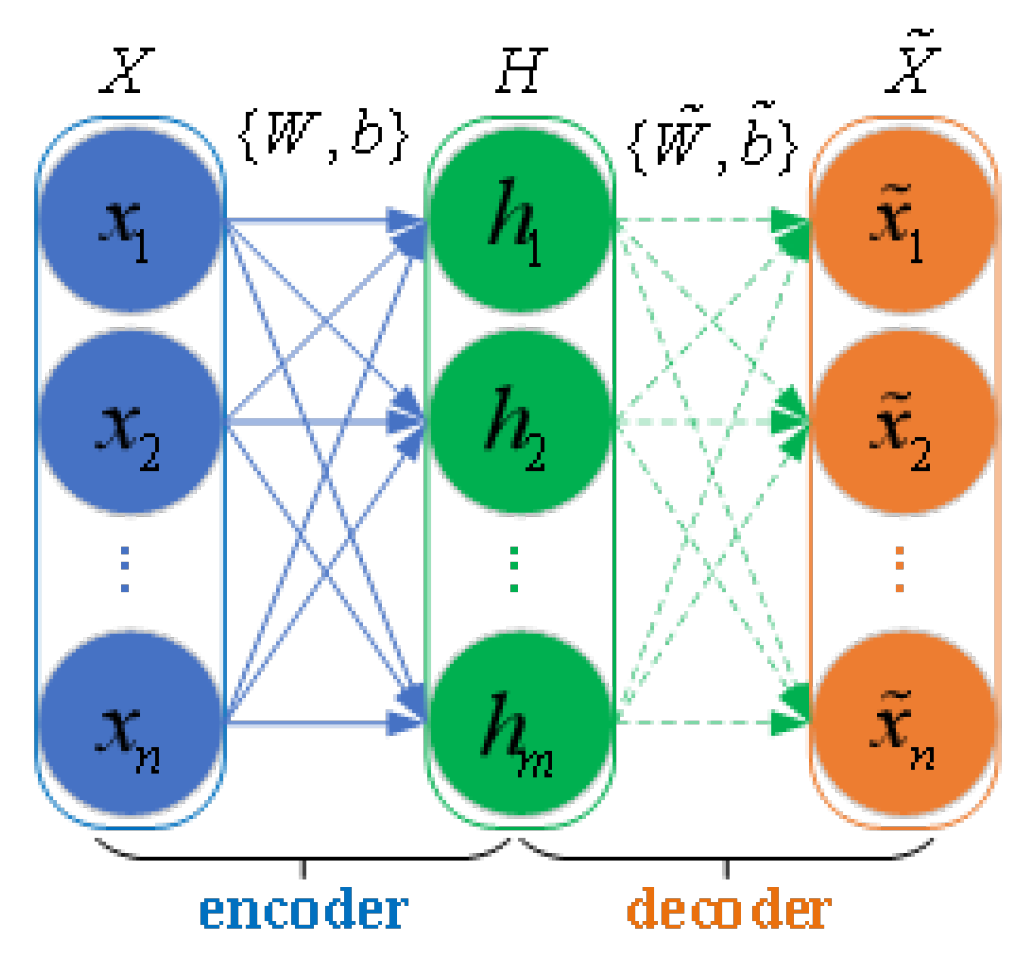
As shown in Figure 2, an Auto-Encoder (AE) [27] is a three-layer neural network which consist of an input layer, a hidden layer, and an output layer. The encoder consists of the input layer and hidden layer, while the decoder includes the hidden layer and output layer. First, the input data are mapped as hidden features in the encoder. Then, the decoder maps the hidden feature to reconstruct the input data at the output layer. The encoder can be represented by
H = f ( W X + b ) ,
where X = x 1 , x 2 , , x n denotes n-dimensional input data, H = h 1 , h 2 , , h m is the hidden information, w and b respectively indicate the weight matrix and bias vector connecting the input layer and hidden layer, and f is the activation function. Similarly, the decoder is expressed as
t i l d e X = f ˜ ( W ˜ H + b ˜ ) ,
where X ˜ = x ˜ 1 , x ˜ 2 , , x ˜ n is the reconstructed output vector, while W ˜ , b ˜ , and f ˜ are the weight matrix, bias vector, and activation function at the output layer, respectively. To train the model parameters and obtain the feature data, the AE is trained using the reconstruction loss function of a mean squared error term, which is J ( X , X ˜ ) = 1 2 n i = 1 n ( x i x ˜ i ) 2 .
In order to further extract key feature information and reduce feature redundancy, the Sparse Auto-Encoder (SAE) proposed in [28] adds a sparse penalty term to the loss function, as follows:
J ( X , X ˜ ) = 1 2 n i = 1 n ( x i x ˜ i ) 2 + β j = 1 h K L ( ρ ρ ^ j )
where is the number of cells in the hidden layer, β is the constant factor of the sparse term, ρ is called the sparse constant, and ρ ^ j is the average activation amount of the j t h cell in the hidden layer, i.e., ρ ^ j = 1 n i = 1 n a j ( x ( i ) ) , where a j ( x ( i ) ) represents the activation amount of the j t h cell in the hidden layer and K L ( ρ ρ ^ j ) is the Kullback–Leibler (KL) divergence. The first term is the Mean Squared Error (MSE) function, while the second term is called the sparse penalty term, which calculates KL divergence value between ρ ^ j and ρ . Specifically, the KL value mathematical expression is provided as follows:
K L ( ρ ρ ^ j ) = ρ ln ρ ρ ^ j + ( 1 ρ ) ln 1 ρ 1 ρ ^ j .
To make most neurons ‘inactive’, the SAE adds a sparse penalty term to let ρ ^ j in a small range during the training process, ensuring that the features of the hidden layer are sparsely distributed.
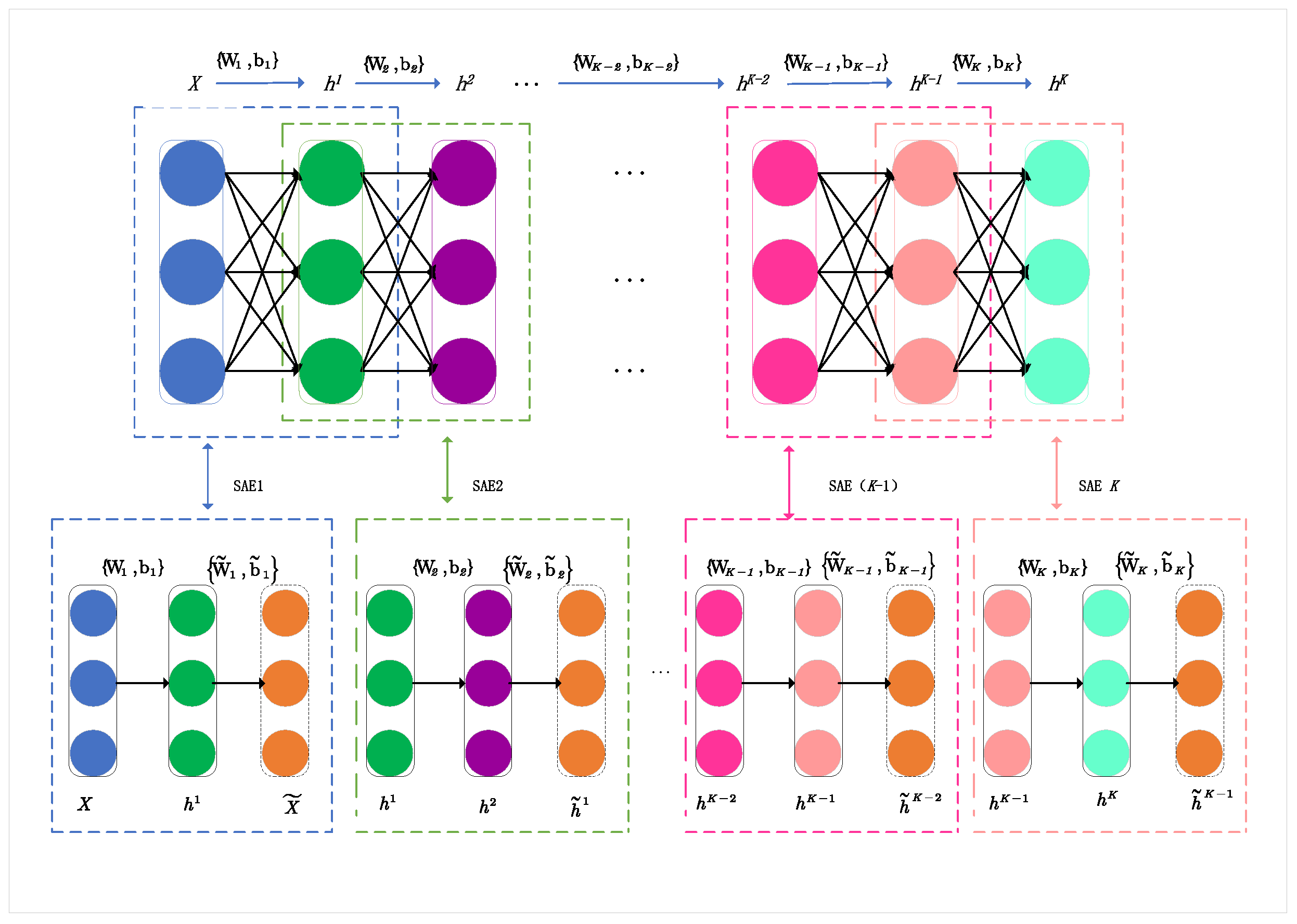
Multiple SAEs can be hierarchically stacked to form a Stacked Sparse Auto-Encoder Network (SSAE). The schematic of an SSAE is illustrated in Figure 3. A deep SSAE network with k layers can be obtained by connecting the encoder part of each SAEs hierarchically, then continuously reconstructing the outputs of the front hidden layers. It should be noted that the decoder part of each SAE is discarded. First, the raw input data X = x 1 , x 2 , , x n and reconstructed data X ˜ = x ˜ 1 , x ˜ 2 , , x ˜ n are utilized to learn the first-layer hidden information h 1 = ( h 1 1 , h 2 1 , , h m 1 ) . Then, the remaining layers of information (h2, h3, …, hK) can be progressively calculated based on layer-wise learning. In SAE1, the encoder maps X to h 1 with parameter set { W 1 , b 1 } and the decoder reconstructs the input data as X ˜ from h 1 with parameters { W ˜ 1 , b ˜ 1 } . In this way, the SSAE can obtain the a multilayer information representation of the original input. For unlabeled data, this can be denoted as h i , i [ 1 , K ] , with the weight and bias parameters of the connection between the hidden layers as { W i , b i } , i [ 1 , K ] . Thus, for situations with insufficient labeled data, SSAE can be used as an unsupervised learning method [29,30].

3. Methodology

The description in Section 2 demonstrates that the complexity of the REEP is closely related to the number of extraction tanks. In this section, the SAE-MBDFFN model is proposed to simulate the REEP with strong coupling and multiple outputs. This model realizes multi-output industrial process simulation by introducing branch output and multiscale feature fusion to meet the changing complexity trend of the REEP. Further, to deal with the lack of labeled data and the issue of models with randomly initialized network parameters easily falling into local optima [14], we use stacked SAE for unsupervised pretraining of SAE-MBDFFN. By introducing SAE to learning the multilayer hidden representation of the original input, which determines the initial values of the network. On the basis of pre-training, supervised fine-tuning of the whole SAE-MBDFFN model can enhance the network generalization.

3.1. Basic Structure of SAE-MBDFFN

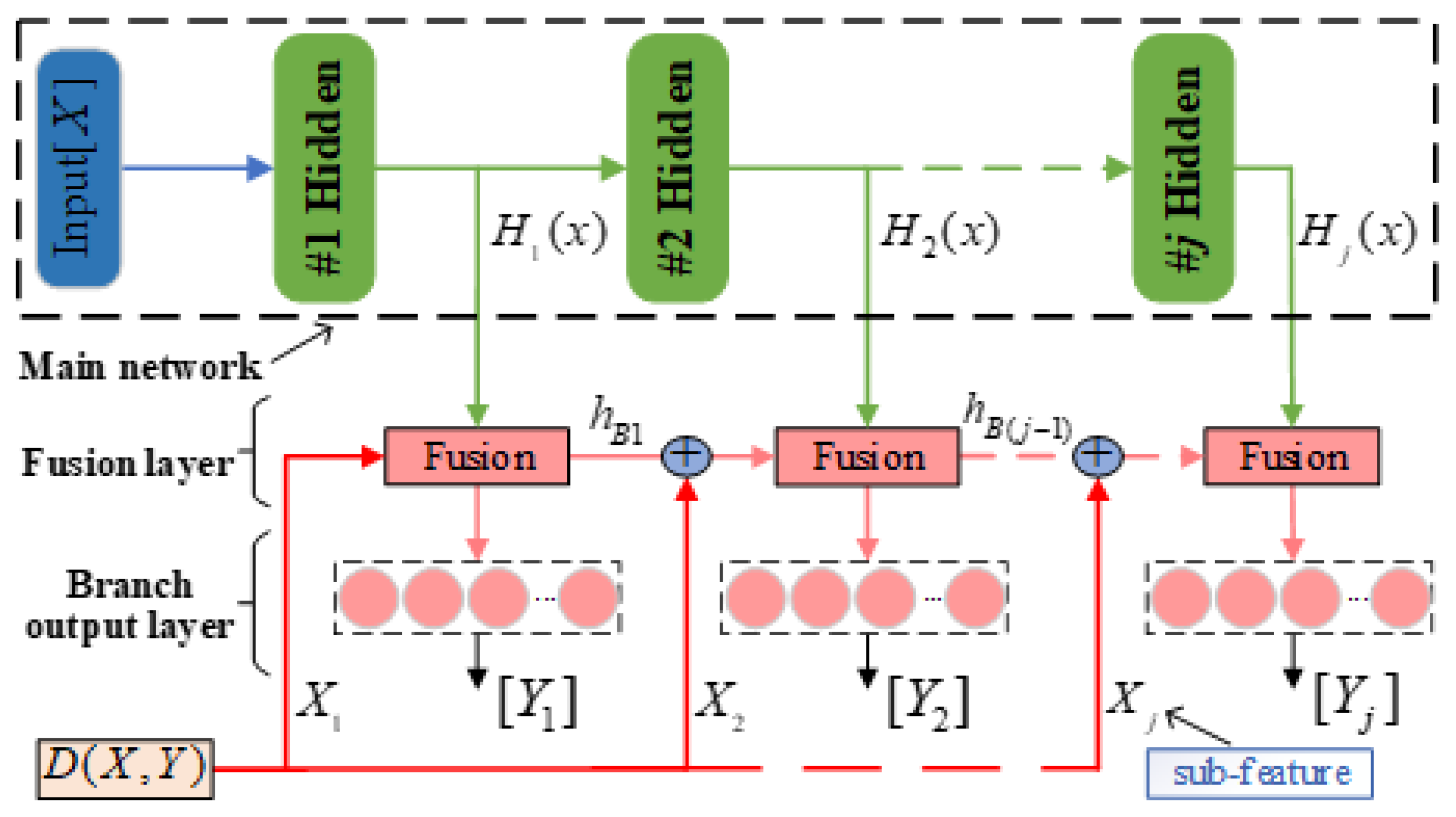
The proposed SAE-MBDFFN consists of a main network, fusion layer, and branch output layer, as shown in Figure 4. Here, X = x 1 , x 2 , , x n represents the input features and Y j   =   [ y j 1 , y j 2 , j [ 1 , n + m ] represents the actual value of the j t h branch. For the complex REEP, we use a multilayer structure to extract the feature information. In SAE-MBDFFN, the component content of the j t h extraction tank is output from the corresponding branch j t h , where the main network formed by stacked SAEs obtains the hidden features H j ( X ) , j [ 1 , n + m ] of the original input based on layer-wise learning.
An actual REEP often involves dozens of extraction tanks. Supposing that the component content of each extraction tank is taken as the branch output, the resulting model will include dozens of hidden layers. This can easily result in gradient disappearance during model training [30]. To address this, SAE-MBDFFN can solves the information loss by introducing multiscale feature fusion. Specifically, a feature fusion layer in each branch of the model extracts the residuals of the original input and the coupled features between branches.
As seen in Figure 4, a branch is designed after each hidden layer in the main network. The branch contains the fusion layer and the output layer for result prediction. In addition to the hidden features H j ( X ) obtained by forward propagation, the subfeature X j and coupled features h B ( j 1 ) of the previous branch are also input to the fusion layer of the j t h branch. First, to transfer more useful information for prediction, we improve upon the traditional residual structure [31,32] by adding an estimate function to calculate the correlation between the original input X and branch output Y j . Then, a subfeature vector X j that contributes more to the output is obtained, where we let X j jump connects to the fusion layer of the j t h branch. To make the subfeatures retain more interpretable information of original features, in this paper we adopt the decision tree regression algorithm [33] as the estimate function, expressed as follows:
X j = D ( X , Y j ) j [ 1 , n + m ] .
Further, it is worth noting that due to the cascade relationship, there is positive coupling between adjacent extraction stages of the REEP (i.e., the component content of the previous extraction tank has an effect on the variation of the component content of the latter extraction tank). To make the model more descriptive of the actual production process, we need to consider this prior information. Thus, we design a branch feature short-connection operation for the n+m-1 branches after branch 1. By feature short-connection, the predicted features extracted in the previous branch can be input to the fusion layer of the next branch, which is called the coupled feature between branches. The details are shown in Figure 4, starting from the second branch fusion layer and adding another feature concatenation before each fusion layer. In this way, the j-th branch fusion layer not only possesses the deep hidden feature H j ( X ) of the main network and residual subfeature X j input, but also the coupled features h B ( j 1 ) from the previous branch.
After forward propagation, SAE-MBDFFN can simultaneously learn the original subfeatures, hidden features, and coupled features between branches in the fusion layer. Therefore, each branch of SAE-MBDFFN can use the features obtained through multiscale fusion to predict the changes in component content. The input vector (predicted feature) of the output layer of the j t h branch is represented as h B ( j 1 ) . After realizing multiscale feature fusion, the input vector of all branch output layers can be expressed as
h B j = H j ( X ) X j , j = 1 , h B j = H j ( X ) h B ( j 1 ) X j , j [ 2 , n + m ] ,
where h B ( j 1 ) denotes the input vector of (j − 1)th branch output layer, H j ( X ) denotes the hidden feature of the j-th hidden layer of main network, and ⊕ represents the concatenation operator. By introducing feature fusion, the branch output function to be learned changes from H j ( X ) to H j ( X ) h B ( j 1 ) X j . This not only improves the prediction accuracy but also alleviates gradient disappearance in the deep neural network. To avoid information loss during feature transfer, in this paper we use concatenation in the feature fusion operation. Let dimensions H j ( X ) h B ( j 1 ) X j be r, s, t, respectively; then, the fused feature dimension obtained by the concatenation operation is dim h B j = r + s + t . In this way, the features of different scales can be extracted and learned simultaneously in the fusion layer of SAE-MBDFFN. The fusion features h B j obtained in the j t h branch are used for making the final prediction of the component content. For the fusion layer and output layer of branch j, the weights and bias parameters of the connection are assumed to be { ω j b , b j b } . Thus, the output expression is Y j = f j ( ω j b h b j + b j b ) , where f j denotes the activation function of the output layer. Similarly, supposing j = n + m, the output of all n + m branches is represented as shown below.
Y 1 = f 1 ( ω 1 b h b 1 + b 1 b ) Y 2 = f 2 ( ω 2 b h b 2 + b 2 b ) Y j = f j ( ω j b h b j + b j b )

3.2. Training Process of SAE-MBDFFN

In REEP, the component content of each extraction tank is difficult to measure in real time, and is usually obtained by offline assay. The offline assay process has a time delay, resulting in incomplete acquisition of the component content under different running conditions. However, the process feature data under different running statuses can be easily collected, which leads to a dataset with two parts: a labeled dataset [ X 1 , Y ] , where X 1 R N 1 × d x is the number of samples, N 1 is the feature dimension (i.e., the number of input features in the sample), and Y = [ y i 1 , y i 2 ] , i [ 1 , n + m ] represents the component content of each extraction tank, and an unlabeled dataset X 2 R N 2 × d x , which generally has N 2 > N 1 due to the ease of data collection. Existing deep learning methods based on supervised training often focus only on datasets with labeled data, ignoring the larger amount of unlabeled feature data. In addition, the typical training process of deep networks adopts random initialization of parameters, which can easily lead to the network falling into local optima. To solve the shortcomings of existing training methods, we propose an unsupervised pretraining method based on stacked SAEs for the parameter initialization of SAE-MBDFFN.
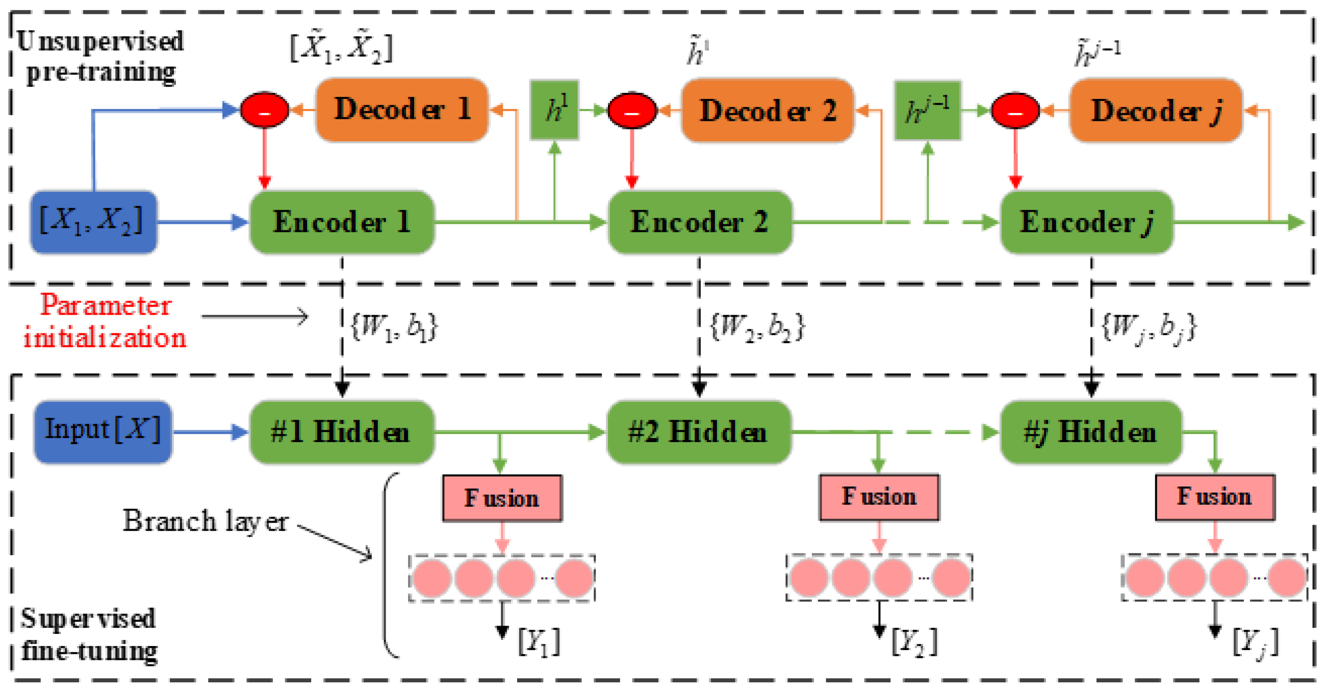
The complete training procedure of SAE-MBDFFN is shown in Figure 5. We define it in two stages: an unsupervised pretraining process using only feature data, and a supervised fine-tuning process using labeled data. In the pretraining stage, a stacked SAE network is constructed with the same number of layers as the SAE-MBDFFN main network. Then, unsupervised training of the stacked SAE uses the feature dataset [ X 1 , X 2 ] . The first SAE structure consists of the input, encoder 1, and decoder 1 layers. First, encoder 1 learns the hidden representation of the input features and outputs its reconstruction [ X ˜ 1 , X ˜ 2 ] to decoder 1. The output vector of encoder 1 is denoted as h 1 . Then, decoder 2 outputs its reconstruction h ˜ 1 obtained by feature extraction to encoder 2. The subsequent process is similar to this. For a deep SAE structure with a total of n+m encoders, the latter SAE reconstructs the encoder output of the previous SAE by minimizing the sparse loss function J ( h j , h ˜ j ) , j [ 1 , n + m ] . In this way, training proceeds layer-wise until the ( n + m ) t h SAE, obtaining a multilayer representation of the original input.
The pretraining process of SAE-MBDFFN does not require labeled data, and hidden information can be learned through the error backpropagation algorithm. After the pretraining, the weight matrix and bias vector parameters of each encoder are expressed as W j , b j , j 1 , n + m . For convenience of display, in Figure 5 we refer to the fusion layer and branch output layer of SAE-MBDFFN together as the branch layer.
After unsupervised pretraining is completed, supervised fine-tuning is carried out. For the stacked SAE network, we remove its decoder parts and retain the (n + m) stacked encoders as the main network of SAE-MBDFFN. On this basis, the SAE-MBDFFN model can be constructed by introducing the branch output after each encoder. The encoder parameter W j , b j , j 1 , n + m obtained during pretraining is the initial parameter of the main network. The labeled dataset [ X 1 , Y ] is then used to fine-tune the whole network. The fine-tuning process needs to first establish the objective loss function of each branch output. In this paper, the MSE function is adopted. For SAE-MBDFFN with branch output, the loss function is represented as follows.
L o s s 1 ( Y 1 , Y ¯ 1 , θ 1 ) = 1 2 N j = 1 N ( Y 1 Y ¯ 1 ) 2 L o s s 2 ( Y 2 , Y ¯ 2 , θ 2 ) = 1 2 N j = 1 N ( Y 2 Y ¯ 2 ) 2 L o s s j ( Y j , Y ¯ j , θ j ) = 1 2 N j = 1 N ( Y j Y ¯ j ) 2
In the above equation L o s s j ( Y j , Y ¯ j , θ j ) , j [ 1 , n + m ] is the loss function of the j t h branch, where N is the total number of training samples, Y j is the actual value of the j t h branch output, and Y ¯ j is the predicted output of the corresponding branch; moreover, θ j = ( W j , b j ) denotes the cumulative weight matrix and bias vector of input to j t h branch. To update the network parameters θ j during the fine-tuning stage, this paper uses the Adam algorithm [16] for iterative training.

3.3. SAE-MBDFFN-Based REEP Simulation

The SAE-MBDFFN method proposed in this paper simulates complex REEPs with strong coupling and multiple outputs through innovative design of a multi-branch structure and multiscale feature fusion mechanism. Further, a pretraining method based on stacked SAEs enables the model to obtain initial parameter values that conform to the actual feature distribution. The training method effectively uses a large amount of unlabeled data while avoiding the shortcomings around local optima encountered with random parameter initialization.
There are four main steps in SAE-MBDFFN-based REEP modeling. First, original data are collected and preprocessed. Second, a stacked SAE network matched with the main network of SAE-MBDFFN is established and the SSAE undergoes layer-wise unsupervised learning via backpropagation. In this step, each encoder can learn the hidden representation of the original feature. Third, the decoder parts of the SSAE network are discarded and the encoder parts are stacked to construct the main network of SAE-MBDFFN, then supervised fine-tuning is performed on the whole model to update all parameters. Lastly, component content is output in each branch layer for the testing samples by substituting only their raw input data into the trained SAE-MBDFFN network and then carrying out forward propagation. The details of the REEP simulation are as follows:
(1)
The feature data [ X 1 , X 2 ] and corresponding labeled data are collected as the original dataset, where Y = [ y i 1 , y i 2 ] , i [ 1 , n + m ] denotes the component content of the organic and aqueous phases in the i t h extraction stage. Then, the network structure of SAE-MBDFFN is determined according to the actual REEP.
(2)
Unsupervised pretraining of the main SAE-MBDFFN network is performed. First, the initial SAE is trained to minimize the reconstruction error between the input data [ X 1 , X 2 ] and reconstructed data [ X ˜ 1 , X ˜ 2 ] . Then, the parameter set [ W 1 , b 1 ] of the first encoder and the hidden feature representation h 1 = h 1 , h 2 , , h L can be obtained, where L represents the number of neurons.
(3)
In a similar way, pretraining of the stacked SAE network is completed by reconstructing the previous encoder’s output in a layer-wise manner. The obtained weight and bias parameter set W j , b j j = 1 , 2 , , n + m are then used the initial parameters of the main network.
(4)
After determining the initial parameters of the main network, the whole SAE-MBDFFN network is fine-tuned based on the labeled dataset [ X 1 , Y ] . The loss function corresponding to the output of each branch is constructed, and the Adam algorithm is used to continuously minimize the output prediction error J j ( Y j , Y ¯ j , θ j ) , j [ 1 , n + m ] . When the loss function converges to around zero, the optimal model in the process is saved and the fine-tuning is considered complete.
(5)
Finally, the model’s prediction accuracy can be evaluated using test data. If the model meets accuracy requirements, it can achieve the purpose of simulating REEP, with the branch output being the component content.
4. Results and Discussion

4.1. Dataset Description

In this section, the proposed method is validated using a 60-stage LaCe/PrNd REE process in Jiangxi Province. The REEP is shown in Figure 1, in which praseodymium and neodymium (i.e., PrNd) are collectively called organic phase products and lanthanum and cerium (i.e., LaCe) are called aqueous phase products. Due to the difficulty of actual data acquisition, it is currently not possible to obtain component content values for all extraction stages. Therefore, we selected five sensitive and representative stages from the 60 extraction stages as the simulation output. These extraction stages can reflect the trend of the whole REEP. Specifically, we used the 15th, 25th, 30th, 35th, and 45th stage, where each stage contains both organic phase and aqueous phase output. The 14 process parameters were taken as the input features, which are described in Table 1. Features x8 and x9 represent export mode and feeding mode, respectively. For x8, 0 means that organic phase is the main product, while 1 means that aqueous phase is the main product. For x9, 0 and 1 mean aqueous phase feed mode and organic phase feed mode, respectively. The simulation platform configuration used in this paper was as follows: OS, Windows 10 (64 bit); CPU, I5-9500K; RAM, 8GB; and implementation using the Tensorflow framework with Python 3.7.
After preprocessing and normalization, 4200 unlabeled samples and 1200 labeled samples were collected. The 4200 unlabeled samples were only used for the unsupervised pretraining based on stacked SAEs. For model fine-tuning and testing in the supervised training stage, 1000 labeled samples were used as the training dataset and the remaining 200 were used for testing. The data distribution curves are shown in Figure 6 for the 14 input features (the blue lines) and the component content of PrNd (organic phase product) in the 30th stage (the red line) of the test dataset.
The Mean Absolute Error (MAE), Root Mean Square Error (RMSE), and coefficient of determination (R2) were used to evaluate the performance of the method, defined as follows:
M A E = 1 N i = 1 N y i y ¯ i
R M S E = 1 N i = 1 N ( y i y ¯ i ) 2
R 2 = 1 i = 1 N ( y i y ¯ i ) 2 i = 1 N ( y i y m e a n ) 2
where N is the total number of test samples, y i and y ¯ i are the real values (label) and prediction values of the i t h test sample, respectively, and y m e a n is the mean of the output values in the testing dataset. Smaller MAE and RMSE values usually indicate good predictive performance for a regression model, while a large R2 value indicates better prediction performance.

4.2. Experimental Setup

Given that there are five extraction stages in which component content variations need to be simulated, we constructed SAE-MBDFFN with five branch outputs. In order to determine the number of neurons in the main network, a grid search was used in the range of [32, 40, 48, 56, 64, 72, 80]. Figure 7 shows the relationship between number of neurons and prediction performance. As shown in Figure 7, the average performance is best when the number of neurons in the main network is 64. Therefore, we set the number of neurons in the main network to 64. In addition, the best number of neurons for the branch output layer was determined to be 32 using a trial-and-error technique. Thus, the main network structure of SAE-MBDFN was [14-64-64-64-64-64] and the structure of each branch was [32-2]. Moreover, a random dropout operation with a dropout rate of 0.5 [34] was introduced to regularize the network.
To assess the performance of SAE-MBDFFN for process simulation, we also tested a Support Vector Machine (SVR) regression model, a BP Neural Network (BPNN) model, a Deep Neural Network (DNN) model with five hidden layers, a Deep Neural Network with pretraining based on SAE (SAE-DNN), and a Multi-Branch Neural Network (MB-DNN) without deep feature fusion. The kernel function of the SVR was the Radial Basis Function (RBF), and the structure of BPNN was [14-64-10]. The DNN and SAE-DNN structure used the same structure as the main network of SAE-MBDFN, except with an output layer added at the end, and both networks used a [14-64-64-64-64-64-10] structure. For MBDNN, the network structure and hyperparameters were the same as those of SAE-MBDFFN. It should be noted that unsupervised pretraining and multiscale feature fusion were not used for MBDNN. Moreover, we adopted the Tanh function as the activation function for the neurons in all of the above neural networks.
For SAE-DNN and SAE-MBDFFN, unsupervised pretraining based on SAE was executed to determine the initial parameters of the hidden layer by feature learning. After pretraining, these networks were trained through supervised fine-tuning, with the learning rate of the neural network set to 10 3 and the Adam algorithm used to optimize the loss function. For the different neural network methods, the batch size was uniformly set to 32 samples. In SAE-MBDFFN, the correlation between the input features and output values was calculated using a decision tree algorithm, after which we selected the top eight features that contributed the most to the output to perform the residual mapping operation. The results of each branch selection are shown in Table 2.

4.3. Experimental Analysis

After pretraining, we analyzed the convergence performance of SAE-MBDFFN during the fine-tuning process. For comparison, the loss curves of DNN, MBDNN, and SAE-MBDFFN are simultaneously shown in Figure 8. It can be easily seen that the initial loss value of the DNN model is the highest, while the initial loss value of MBDNN with a branch structure is lower. This indicates that the branch structure is more suitable for multiple-output process simulation even when random parameter initialization is adopted. Further, the convergence performance of our proposed SAE-MBDFFN is the best compared to DNN and MBDNN. Figure 8 shows that SAE-MBDFFN not only has the lowest initial loss value but can also reach the convergence state very quickly.
The aforementioned six models were trained and utilized to simulate the component contents in the test dataset. The prediction evaluation indicators of the six methods are shown in Figure 9a–c, where we distinguish the results for the organic and aqueous phases. As can be seen from Figure 9, the two shallow models, SVR and the BPNN, have the worst simulation performance; this is because shallow models do not have enough learning capacity to simulate REEPs with increasing complexity by stages. Hence, the DNN model with multiple layers clearly outperforms both shallow models in terms of MAE, RMSE, and R2. However, as this DNN does not previously extract the hidden information of unlabeled data, it cannot achieve the best performance when training is based on insufficient labeled data. Further, we adopted an unsupervised pretraining method based on stacked SAEs for DNN parameter initialization. Compared with random parameter initialization, it can be seen from Figure 9 that the prediction performance of the resulting SAE-DNN is further improved. This indicates that pretraining is beneficial for REE process simulation.
It is worth noting that the SAE-DNN is only a one-way transfer network, and has no structure designed for the actual characteristics of REEPs. This means that when the hidden layer learns the wrong features, SAE-DNN preserves them during training, leading to unstable prediction results. The neural network model that we propose in this paper addresses this problem by incorporating multiple branch outputs for REEP simulations. For this comparison, we did not use unsupervised pretraining methods or deep feature fusion mechanisms for MBDNN. As can be seen in Figure 9a–c, the prediction performance of MBDNN is better than that of SAE-DNN for both the organic and aqueous phases. Unlike both these models, our proposed SAE-MBDFFN can concatenate the original features and inter-branch coupled features in its branch fusion layer. In addition, SAE-MBDFFN fully learns useful information for prediction through two stages, namely, unsupervised pretraining and fine-tuning. These results show that SAE-MBDFFN achieves the best performance compared to the other methods. Our method achieves the lowest values of MAE and RMSE and highest R2 values for for both organic and aqueous phases at each extraction stage.
To further compare the different methods, we calculated the means of the evaluation indicators for the five extraction stages, as shown in Figure 9. The results are presented in Table 3, with the optimal values in bold. From the MAE, RMSE, and R2 results, it can easily be seen that SVR and BPNN perform the worst among the six models on average. By adopting a multilayer network structures, the DNN models can simulate complex relationships in the data more accurately than SVR and BPNN; however, for the traditional DNN, the parameters of the hidden layer are randomly initialized, making it prone to local optima. SAE-DNN addresses this by using a layer-wise unsupervised pretraining method based on stacked SAEs to determine the initial parameters of the DNN, allowing it to learn the hidden representations of unlabeled data as initial parameters during pretraining. This can help the network to avoid falling into local optima during the fine-tuning phase. As expected, the results show that the average prediction performance of the SAE-DNN model is better than that of the traditional DNN.
Although the MAE, RMSE, and R2 values of SAE-DNN for organic phase improve to 0.0295, 0.0422, and 0.9270, respectively, compared to the traditional DNN, SAE-DNN remains insufficient for REEP simulations that require high accuracy. To address this, the MBDNN model includes a multi-branch output structure. According to Table 3, the simulation accuracy of MBDNN is significantly better than that of SAE-DNN, which illustrates the effectiveness of the branch structure for nonlinear multiple-output processes. Finally, our proposed SAE-MBDFFN model introduces a feature fusion layer with a residual structure and branch feature short-connection. In addition, the initial values of the network parameters are determined through the unsupervised SAE pretraining method, which further improves the performance of SAE-MBDFFN. From the table, it can be seen that the MAE, RMSE, and R2 values of SAE-MBDFFN are optimal in both the aqueous phases and organic phases, showing the best performance among all six methods.
Considering that the extraction tank located in the middle section has more frequent reaction changes during the production process, we show the detailed prediction results of the SAE-DNN, MBDNN, and SAE-MBDFFN models for the 30th stage in Figure 10 for a better illustration, In the figure, ACC stands for the aqueous-phase component content and OCC for the organic-phase component content. As the figure shows, the three models can all predict the basic change trend of the component content; however, some data points of SAE-DNN and MBDNN obviously have large deviations from the actual values. If such deviations with large errors are used as simulation results, they may interfere with correct decision-making during the production process. On the other hand, the proposed SAE-MBDFFN model maximally fits the actual values and has the best prediction accuracy among the models. SAE-MBDFFN has a multi-branch structure that corresponds to the reaction order of REEP, which is used to learn the distribution relationships of the process data. In addition, unsupervised pretraining is adopted to determine the initial parameters of the hidden layer and achieve deep multiscale feature fusion in the fine-tuning stage. These experimental results show the effectiveness of the proposed SAE-MBDFFN method for process simulation.
Finally, the simulation effectiveness of the proposed method for REEP is verified by randomly selecting six test samples. The simulation results of SAE-MBDFFN are shown in Figure 11a–f, where ECC stands for element component content. It can be seen from each figure that the proposed method can accurately simulate the variation in the actual composition content and that the distribution of the numerical error is within an acceptable range. Thus, simulation results provided by SAE-MBDFFN can be utilized as decision support for process adjustment of REEPs.

5. Conclusions

In this paper, we have proposed a novel multi-branch deep network for REEP modeling, which we call SAE-MBDFFN. The proposed model can predict the component content of REEs more reliable by introducing a feature fusion layer in each branch. First, the hidden features, original features, and inter-branch coupled features are used in combination to predict the component content. Second, to address the issue of limited labeled data, an unsupervised pretraining method based on a Sparse Auto-Encoder (SAE) is proposed. For the SAE, layer-wise information reconstruction in the pretraining stage is used to initialize the parameters of the hidden layer and constrain the data distribution, helping the network to reach the global optimum. We validated the proposed method on a real industrial dataset. Our experiment results showed that the proposed method outperforms other models used for comparison, including traditional data-driven models and deep models without pretraining. Future work could focus on the interpretability of the model, which would allow for the extension of methods based on SAE-MBDFFN to other process industries with multiple outputs and strong coupling.

Author Contributions

Conceptualization, J.Z.; data curation, W.W.; funding acquisition, J.Z.; methodology, J.Z.; resources, F.X.; software, W.W.; supervision, J.Z.; writing—review and editing, F.X. All authors have read and agreed to the published version of the manuscript.

Funding

This research was supported by the National Natural Science Foundation of China under Grant 62363010, the Open Research Project of the State Key Laboratory of Industrial Control Technology of China under Grant ICT2024B50, and the National Natural Science Foundation of China under Grant 61991404.

Data Availability Statement

The data presented in this study are available on request from the corresponding author.

Conflicts of Interest

The authors declare no conflicts of interest.

References

  1. Zhang, L.Y.; Minghui, H.B. Study on the leaching behavior of rare earths and fluoride in NdCl3-MgF2 (CaF2)—HCl solution system. Chin. J. Rare Earth 2024, 10, 1–13. [Google Scholar]
  2. Balaram, V. Rare earth elements: A review of applications, occurrence, exploration, analysis, recycling, and environmental impact. Geosci. Front. 2019, 10, 1285–1303. [Google Scholar] [CrossRef]
  3. Liao, C.C.; Cheng, F.X.; Wu, S.; Yan, C. Review and recent progresses on theory of countercurrent extraction. J. Chin. Soc. Rare Earths 2017, 35, 1–8. [Google Scholar]
  4. Yang, H.; Xu, Y.; Wang, X. Component Content Soft-Sensor Based on RBF Neural Network in Rare Earth Countercurrent Extraction Process. In Proceedings of the 2006 6th World Congress on Intelligent Control and Automation, Dalian, China, 21–23 June 2006; IEEE: Piscataway, NJ, USA, 2006; Volume 1, pp. 4909–4912. [Google Scholar]
  5. Dai, W.; Yang, H.; Lu, R.; Zhu, J.; Chen, P. Optimization Setting of Reagent Dosage in Rare Earth Extraction Process Based on JITL. In Proceedings of the 2022 4th International Conference on Industrial Artificial Intelligence (IAI), Shenyang, China, 24–27 August 2022; IEEE: Piscataway, NJ, USA, 2022; pp. 1–6. [Google Scholar]
  6. Zhong, X. Study on effective separation factor for multi-component rare earths in counter-current extraction. Rare Earths 2009, 30, 57–60. [Google Scholar]
  7. Ding, Y.; Zhong, L.; Yang, H. Static optimization design study of two outlets cascade extraction for any component. J. Chin. Soc. Rare Earths 2010, 28, 53. [Google Scholar]
  8. Yun, C.Y.; Lee, C.; Lee, G.G.; Jo, S.; Sung, S.W. Modeling and simulation of multicomponent solvent extraction processes to purify rare earth metals. Hydrometallurgy 2016, 159, 40–45. [Google Scholar] [CrossRef]
  9. Yuan, X.; Zhou, J.; Huang, B.; Wang, Y.; Yang, C.; Gui, W. Hierarchical quality-relevant feature representation for soft sensor modeling: A novel deep learning strategy. IEEE Trans. Ind. Inform. 2019, 16, 3721–3730. [Google Scholar] [CrossRef]
  10. Sun, Q.; Ge, Z. A survey on deep learning for data-driven soft sensors. IEEE Trans. Ind. Inform. 2021, 17, 5853–5866. [Google Scholar] [CrossRef]
  11. Giles, A.; Aldrich, C. Modelling of rare earth solvent extraction with artificial neural nets. Hydrometallurgy 1996, 43, 241–255. [Google Scholar] [CrossRef]
  12. Anitha, M.; Singh, H. Artificial neural network simulation of rare earths solvent extraction equilibrium data. Desalination 2008, 232, 59–70. [Google Scholar] [CrossRef]
  13. Ma, Y.; Stopic, S.; Gronen, L.; Milivojevic, M.; Obradovic, S.; Friedrich, B. Neural network modeling for the extraction of rare earth elements from eudialyte concentrate by dry digestion and leaching. Metals 2018, 8, 267. [Google Scholar] [CrossRef]
  14. Erhan, D.; Courville, A.; Bengio, Y.; Vincent, P. Why does unsupervised pre-training help deep learning? In Proceedings of the Thirteenth International Conference on Artificial Intelligence and Statistics, JMLR Workshop and Conference Proceedings, Sardinia, Italy, 13–15 May 2010; pp. 201–208. [Google Scholar]
  15. Zheng, S.; Zhao, J. A new unsupervised data mining method based on the stacked autoencoder for chemical process fault diagnosis. Comput. Chem. Eng. 2020, 135, 106755. [Google Scholar] [CrossRef]
  16. Yuan, X.; Ou, C.; Wang, Y.; Yang, C.; Gui, W. A novel semi-supervised pre-training strategy for deep networks and its application for quality variable prediction in industrial processes. Chem. Eng. Sci. 2020, 217, 115509. [Google Scholar] [CrossRef]
  17. Zhao, X.; Jia, M.; Liu, Z. Semisupervised deep sparse auto-encoder with local and nonlocal information for intelligent fault diagnosis of rotating machinery. IEEE Trans. Instrum. Meas. 2020, 70, 3501413. [Google Scholar] [CrossRef]
  18. Yang, H.; He, L.; Zhang, Z.; Lu, R.; Tan, C. Multiple-model predictive control for component content of CePr/Nd countercurrent extraction process. Inf. Sci. 2016, 360, 244–255. [Google Scholar] [CrossRef]
  19. Xiang, Z.; Liu, S. Component content soft-sensor in rare-earth extraction based on PSO and LS-SVM. In Proceedings of the 2008 Fourth International Conference on Natural Computation, Jinan, China, 18–20 October 2008; IEEE: Piscataway, NJ, USA, 2008; Volume 6, pp. 392–395. [Google Scholar]
  20. Teerapittayanon, S.; McDanel, B.; Kung, H.T. Branchynet: Fast inference via early exiting from deep neural networks. In Proceedings of the 2016 23rd International Conference on Pattern Recognition (ICPR), Cancun, Mexico, 4–8 December 2016; IEEE: Piscataway, NJ, USA, 2016; pp. 2464–2469. [Google Scholar]
  21. Ou, Z.X.; Yu, B.Y.W. An Efficient Algorithm-Hardware Co-Design for Radar-Based Fall Detection With Multi-Branch Convolutions. IEEE Trans. Circuits Syst. I Regul. Pap. 2023, 70, 1613–1624. [Google Scholar] [CrossRef]
  22. Chen, H.; Lagadec, B.; Bremond, F. Partition and reunion: A two-branch neural network for vehicle re-identification. In Proceedings of the CVPR Workshops, Long Beach, CA, USA, 15–20 June 2019; pp. 184–192. [Google Scholar]
  23. Tan, Y.; Liu, M.; Chen, W.; Wang, X.; Peng, H.; Wang, Y. DeepBranch: Deep neural networks for branch point detection in biomedical images. IEEE Trans. Med. Imaging 2019, 39, 1195–1205. [Google Scholar] [CrossRef]
  24. Wang, Q.; Wang, K.; Li, Q.; Yang, Z.; Jin, G.; Wang, H. MBNN: A multi-branch neural network capable of utilizing industrial sample unbalance for fast inference. IEEE Sens. J. 2020, 21, 1809–1819. [Google Scholar] [CrossRef]
  25. Yang, Z.; Baraldi, P.; Zio, E. A multi-branch deep neural network model for failure prognostics based on multimodal data. J. Manuf. Syst. 2021, 59, 42–50. [Google Scholar] [CrossRef]
  26. Xu, D.; Shi, Y.; Tsang, I.W.; Ong, Y.S.; Gong, C.; Shen, X. Survey on multi-output learning. IEEE Trans. Neural Netw. Learn. Syst. 2019, 31, 2409–2429. [Google Scholar] [CrossRef]
  27. Liu, Y.; Liu, B.; Zhao, X.; Xie, M. Development of RVM-based multiple-output soft sensors with serial and parallel stacking strategies. IEEE Trans. Control Syst. Technol. 2018, 27, 2727–2734. [Google Scholar] [CrossRef]
  28. Wang, Y.; Yao, H.; Zhao, S. Auto-encoder based dimensionality reduction. Neurocomputing 2016, 184, 232–242. [Google Scholar] [CrossRef]
  29. Wen, L.; Gao, L.; Li, X. A new deep transfer learning based on sparse auto-encoder for fault diagnosis. IEEE Trans. Syst. Man Cybern. Syst. 2017, 49, 136–144. [Google Scholar] [CrossRef]
  30. Wu, Y.; Liu, D.; Yuan, X.; Wang, Y. A just-in-time fine-tuning framework for deep learning of SAE in adaptive data-driven modeling of time-varying industrial processes. IEEE Sens. J. 2020, 21, 3497–3505. [Google Scholar] [CrossRef]
  31. He, K.; Zhang, X.; Ren, S.; Sun, J. Identity mappings in deep residual networks. In Proceedings of the Computer Vision–ECCV 2016: 14th European Conference, Proceedings, Amsterdam, The Netherlands, 11–14 October 2016; Part IV 14. Springer: Berlin/Heidelberg, Germany, 2016; pp. 630–645. [Google Scholar]
  32. Boroumand, M.; Chen, M.; Fridrich, J. Deep residual network for steganalysis of digital images. IEEE Trans. Inf. Forensics Secur. 2018, 14, 1181–1193. [Google Scholar] [CrossRef]
  33. Torres-Barrán, A.; Alonso, Á.; Dorronsoro, J.R. Regression tree ensembles for wind energy and solar radiation prediction. Neurocomputing 2019, 326, 151–160. [Google Scholar] [CrossRef]
  34. Srivastava, N.; Hinton, G.; Krizhevsky, A.; Sutskever, I.; Salakhutdinov, R. Dropout: A simple way to prevent neural networks from overfitting. J. Mach. Learn. Res. 2014, 15, 1929–1958. [Google Scholar]
Figure 1. Diagram of RE cascade extraction process.
Processes 12 02861 g001
Figure 2. A SAE network.
Processes 12 02861 g002
Figure 3. Schematic of SSAE network with K encoders; the blue circles indicate data neurons from the original input, the orange circles are reconstructed data neurons, and the other color circles are hidden feature neurons.
Processes 12 02861 g003
Figure 4. Structure of SAE-MBDFFN.
Processes 12 02861 g004
Figure 5. The unsupervised pretraining and fine-tuning procedure of SAE-MBDFFN.
Processes 12 02861 g005
Figure 6. Data trend plots for feature variables and output y(30)1.
Processes 12 02861 g006
Figure 7. Grid search of hidden layer neurons.
Processes 12 02861 g007
Figure 8. The loss change curve of fine-tuning.
Processes 12 02861 g008
Figure 9. Comparison of MAE, RMSE, and R2 results for the different methods: (a) MAE, (b) RMSE, and (c) R2.
Processes 12 02861 g009
Figure 10. Comparison of prediction fitting results for the 30th extraction stage.
Processes 12 02861 g010
Figure 11. Process simulation results of SAE-MBDFFN for test samples: (a) first sample simulation, (b) 35th sample simulation, (c) 50th sample simulation, (d) 105th sample simulation, (e) 142nd sample simulation, (f) 183rd sample simulation.
Processes 12 02861 g011
Table 1. Description of input features.
No.Feature Meaning Description
x1La element composition in feed liquid
x2Ce element composition in feed liquid
x3Pr element composition in feed liquid
x4Nd element composition in feed liquid
x5Ce/La separation factor
x6Pr/Ce separation factor
x7Nd/Pr separation factor
x8Main product export mode
x9Feeding mode
x10Amount of extracting solvent
x11Amount of scrubbing solvent
x12Feeding stage
x13Organic phase export fraction
x14Aqueous phase outlet fraction
Table 2. Subfeature select results of each branch.
No. BranchFeature Select Results
branch 1x1, x5, x7, x10, x11, x12, x13, x14
branch 2x1, x2, x4, x9, x10, x12, x13,x14
branch 3x1, x2, x3, x6, x10, x12, x13, x14
branch 4x1, x2, x3, x6, x10, x12, x13, x14
branch 5x2, x3, x6, x7, x10, x11, x13, x14
Table 3. Average performance of the different methods.
MethodPhaseMAERMSER2
SVROrganic0.05600.06660.7890
Aqueous0.05740.07170.8510
BPNNOrganic0.04280.05730.8475
Aqueous0.05690.07620.8277
DNNOrganic0.03460.04810.8912
Aqueous0.04170.06100.8910
SAE-DNNOrganic0.02950.04220.9270
Aqueous0.03650.05460.9118
MBDNNOrganic0.02550.03750.9427
Aqueous0.03040.04720.9342
SAE-MBDFNOrganic0.01540.02440.9751
Aqueous0.01960.03250.9675
Disclaimer/Publisher’s Note: The statements, opinions and data contained in all publications are solely those of the individual author(s) and contributor(s) and not of MDPI and/or the editor(s). MDPI and/or the editor(s) disclaim responsibility for any injury to people or property resulting from any ideas, methods, instructions or products referred to in the content.