Evaluation of Mixing Process in Batch Mixer Using CFD-DEM Simulation and Automatic Post-Processing Method

Abstract

A batch mixer is an important piece of equipment for polymer filling modification, and the kinematics of agglomerate breakup and distribution are necessary for the structure design and mixing process optimization of the rotor, particularly in light of the cohesive forces that exist within the agglomerate. In this paper, computational fluid dynamics (CFD) was coupled with discrete element method (DEM) to simulate the mixing process, including breakup and distribution, which was further quantitatively evaluated by the post-processing involving numerical method. To study the mixing process of an agglomerate composed of massive spherical particles (individual particle ratio was r), the coordinates of the particles were exported from the CFD-DEM simulation results. Then, the coordinate data were automatically processed with an automate custom-built post-processing program to obtain the average radius of gyration (R_gy) and the particle distribution density (ε). The kinematics analyzation of breakup and distribution was represented by curve of R_gy/r versus mixing time (t) and curve of ε versus t, respectively. The value of R_gy/r and ε decreased over time until they reached an equilibrium and vibrated around a certain value. In particular, a notable decline in the value of R_gy/r was observed following an increase prior to critical time. The increase in R_gy/r stated that the agglomerate or aggregates undergo stretching deformation. Additionally, mixing processes of rotors with different pressurization coefficients (S) and rotation speeds could be facilitated and intensified by large S and high rotation speed. Finally, a “breakup-line” was developed by considering the influence of cohesive force and rotation speed on the agglomerate breakup process. The agglomerate could be broken if the combination of rotation speed and bonding strength was above the “breakup line”, otherwise the agglomerate was not broken. Furthermore, rotors with larger slopes exhibited stronger breakup ability.

1. Introduction

It is common that the composites’ performance relies on the dispersive and distributive state of filler particles [1,2], while large-sized agglomerates are usually formed in filler powder owing to the cohesive force between particles, such as van der Waals force [3,4]. The batch mixer or twin-screw extruder is the primary equipment for breaking up the agglomerate in melt polymer, realizing desired filler dispersion and distribution for preparing the composites with well performance. Owing to the complex configuration of equipment and the un-transparent polymer melt, evaluating the mixing process and modeling the kinematics in equipment are difficult for filling modification.

To study the break process, convenient and low-cost computational fluid dynamics (CFD) simulation has been developed, which provides a comprehensive and authentic analysis of the flow field and mixing ability in equipment. Manas-Zlockzower [5,6,7] has performed numerous experimental and CFD simulation studies, and proved that erosion is an important dispersive mechanism for polymer modification. Potente [8] modeled the dispersion process of spherical agglomerate in polymer melt. Hosseini [9] utilized CFD to simulate the erosion-driven fragmentation of small-sized agglomerates. Guo Jiang [10] examined the influence of chaotic mixing on the rheological behavior and microstructure of polypropylene (PP)/clay nanocomposites through numerical simulation, and the results indicated that promoting higher strain is crucial for superior properties of polymer/clay nanocomposites. However, the CFD simulations mentioned above are usually limited to analyzing the flow field, and the effect of flow on filler’ dispersion and distribution is always studied with tracer particles, which are treated as a continuous solid phase without considering mass and cohesive force. Thus, CFD simulation cannot reflect the dispersion and distribution process of agglomerate in equipment as realistically as possible.

Discrete element method (DEM) is a method for analyzing powder movement and dispersion in conveying process, particularly for discontinuous materials. The most important is that DEM simulation can be coupled with CFD to study the flow effect on particles. The intensification process of gas-solid fluidization processes in a gas-solid vortex unit (GSVU) [11], hydraulic transport of coarse particles [12] and fluid dynamics of jet fluidized bed [13] had been modeled and researched by CFD coupling with DEM (CFD-DEM). However, the fluid-solid complex processes mentioned above is predominantly associated with low-viscosity fluids. As for the mixing process in mixer or extruder, viscosity of melt polymer is relatively high, and the high viscous flow can impose greater effect on agglomerates’ breakup and distribution process. In recent years, Graziano Frungieri [14] had done some pioneer works in studying the breakup process in batch mixer with CFD-DEM simulation method, but the distribution process is not discussed.

In existing works, characterize parameters and methods have been developed to evaluate the mixing process. The most widely used parameters in characterizing the dispersion ability are shear stress, shear rate and mixing index [15,16]. Length of stretch, instantaneous efficiency and time average efficiency, deduced by Ottino [17] are useful for characterizing the flow stretching and distribution ability. Danckwerts [18] report that average size of segregated regions in mixer could be represented by the scale of segregation, which could be applied to evaluate the distribution mixing. To reveal the relation between flow pattern structure and the geometry of screw elements, Yssuya Nakayama [19] proposed the distribution of volumetric strain rate to characterize the strain rate for general flow in extruder or mixer. These parameters proposed with post-processing results of CFD simulation are useful in understanding the flow field and mixing ability. Besides, the post-processing results of CFD simulation result always give a general evaluation for mixing process. To deeply reveal the mixing process, especially for the breakup and distribution, the kinematics should be modeled [20,21].

To perform the kinematics analyzation of mixing process, the quantitative evaluation for breakup and distribution are required. In CFD-DEM simulation, the agglomerate is always composed of numerous particles, and will be broken up into smaller aggregates or mono-dispersed particles, which are distributed in flow domain. Thus, describing the breakup and distribution state at different mixing time is essential. Inspired by reported studies [14,22,23] average radius of gyration (R_gyA) and particle distribution density (ε) show promising potential for quantitatively describing the mixing state at different time. However, there are large amount of data in simulation results, so the convenient and automatic post-processing method also need to be established. The purpose of this paper is to analyze the kinematics of breakup and distribution in batch mixer using CFD-DEM simulation. At first, a post-processing method is established to automatically calculate the R_gyA and ε, respectively, which are used to describe the breakup and distribution state at different mixing time. Then, curves for the R_gyA/r (r is the particle radius) and ε changing with mixing time are drawn, which is used to evaluate mixing process and perform the kinematics analyzation. Furthermore, the mixing processes of rotors with different configurations and rotating speeds are simulated. Pressurization coefficient (S) is used to represent the rotor configuration. And the influence of S and rotating speed on breakup and distribution is evaluated and compared. Finally, a “breakup-line” considering that the cohesive force and rotating speed is modeled to judge the breakup of agglomerate during mixing.

2. CFD-DEM Coupling Simulation

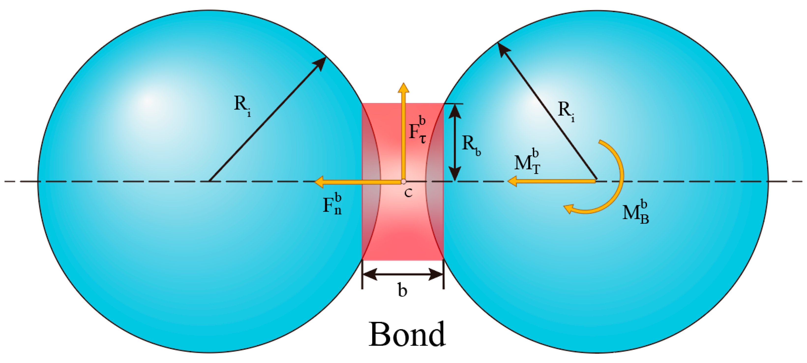
2.1. Cohesive Force Model

Cohesive force between particles is often described by contact models, which can be divided into two main types: cohesive contact models and adhesive contact models. Cohesive contact models usually refer to particle-particle interactions caused by forces such as van der Waals force or liquid bridge. Although these models possess finite contact areas, the contribution to the torsion or bending resistance of the contact is usually neglected, particularly in cohesive systems [13]. It is worth mentioning that adhesive contact forms during bond initiation, and is irreversibly removed upon break. Bonded contact models commonly employ for bonded systems incorporate mechanisms for bending and torsional resistance [24,25], which can describe the interaction forces between calcium carbonate fillers [26,27,28,29]. Figure 1 presents an adhesive contact model proposed by Potyondy and Sangrós [24,30], and the model envisioned as two particles connecting with each other with a massless cylindrical “bond”, which allowing the deformation of elastic and viscous forces and moments that are caused by relative motion among particles. Once the external force exceeds bonding strength, the bonding between the particles will be broken.

The bond in the model will exert an elastic force on both bonded particles to oppose the linear deformation s^bond, the normal and tangential components of this force will be given as:

$$F_n^{bond,e}=-K_n^{″}{A}_{bond}{s}_n^{bond}$$

(1)

$$F_{\tau }^{bond,e}=-K_{\tau }^{″}{A}_{bond}{s}_{\tau }^{bond}$$

(2)

$$A_{bond}=\pi R_{bond}^2$$

(3)

$K_{\mathsf{\tau }}^{″}$ and $K_n^{″}$ are tangential and normal stiffnesses per unit area, respectively. $A_{\mathit{bond}}$ is cross-sectional area of the bond${ s}_n^{\mathit{bond}}$, and${ s}_{\mathsf{\tau }}^{\mathit{bond}}$ are normal and tangential components of the bond’s linear deformation $s^{\mathit{bond}}$, respectively.

The normal component of angular deformation vector (${\theta }_n^{\mathit{bond}}$) represents torsional deformation, while tangential component (${\theta }_{\mathsf{\tau }}^{\mathit{bond}}$) characterizes the bond bending. The corresponding torsional and bending components of the moment ($M_T^{\mathit{bond}}$, $M_B^{\mathit{bond}}$) that oppose to those angular deformations are calculated as:

$$M_T^{bond}=-K_{\tau }^{″}{J}_{bond}{\theta }_n^{bond}$$

(4)

$$M_B^{bond}=-K_n^{″}{I}_{bond}{\theta }_{\tau }^{bond}$$

(5)

$J_{\mathit{bond}}$ and${ I}_{\mathit{bond}}$ are inertia moments for polar and bond’s cross-section. In addition to the elastic forces and moments described above, viscous forces and moments are also exerted for reducing oscillations that may arise between bonded particles. The normal and tangential components are calculated using the following expressions:

$$F_n^{bond,v}=-2{\eta }_{bond}\sqrt{K_n^{"}{A}_{bond}{m}^{*}}{v}_n^{rel}$$

(6)

$$F_{\tau }^{bond,v}=-2{\eta }_{bond}\sqrt{K_{\tau }^{"}{A}_{bond}{m}^{*}}{v}_{\tau }^{rel}$$

(7)

$$M_T^{bond,v}=-2{\eta }_{bond}\sqrt{K_{\tau }^{"}{A}_{bond}{m}^{*}}{\displaystyle \frac{J_{bond}}{A_{bond}}}{\omega }_n^{rel}$$

(8)

$$M_B^{bond,v}=-2{\eta }_{bond}\sqrt{K_n^{"}{A}_{bond}{m}^{*}}{\displaystyle \frac{I_{bond}}{A_{bond}}}{\omega }_{\tau }^{rel}$$

(9)

η_bond is damping ratio attributed to the bond. $m^{*}$ is equivalent mass of the pair particles in Figure 1 $v_n^{\mathit{vel}}$ and $v_{\mathsf{\tau }}^{\mathit{vel}}$ are normal and tangential components of the relative velocity vector defined by equation. ${\omega }_n^{\mathit{vel}}$ and ${\omega }_{\mathsf{\tau }}^{\mathit{vel}}$ are normal and tangential components of the relative rotational velocity vector.

2.2. DEM Control Equations

In DEM, translational and rotational particles are controlled by solving explicitly Euler’s first and second laws. All particles within the computational domain are tracked in Lagrangian way:

$$m_{particle}{\displaystyle \frac{d{v}_{particle}}{dt}}=F_{n,\tau }^{bond,e}+F_{fluid\to particle}+m_{particle}g$$

(10)

$$F_{fluid\to particle}=-V_p\nabla p+{\displaystyle \frac{1}{2}}{C}_D{\rho }_{fluid}{A}^{\prime }\left|u-v_p\right|\left(u-v_p\right)$$

(11)

$$J_{particle}{\displaystyle \frac{d{\omega }_{particle}}{dt}}=M_c+M_{fluid\to particle}$$

(12)

where $m_{\mathit{particle}}$ is particle mass, g is gravitational acceleration vector, $F_c$ is contact force that accounts for particle-particle and particle-wall interactions, ${\omega }_{\mathit{particle}}$ is angular velocity vector, $J_{\mathit{Particle}}$ is moment of inertia tensor, $M_c$ is net torque generated by tangential forces causing particle rotation, $F_{\mathit{fluid}\to \mathit{particle}}$ is additional force accounting for the interaction with the fluid phase, and $M_{\mathit{fluid}\to \mathit{particle}}$ is additional torque due to fluid phase velocity gradient. Furthermore, Di Felice [31] derived a correction function for considering the case of dense particle flows. The correlation is given by:

$$C_D=C_{D_0}{\alpha }_f^{2-\zeta }$$

(13)

$C_{D_0}$ is the drag coefficient for a single particle, which is calculated using the particle’s Reynolds number based on the superficial relative velocity, ${\alpha }_f$ stands for fluid volume fraction. The ζ is calculated by:

$$\zeta =3.7-0.65exp\left\{-{\displaystyle \frac{1}{2}}{\left[1.5-lo{g}_{10}({\alpha }_{f}R{e}_p)\right]}^2\right\}$$

(14)

2.3. CFD Control Equations

The isothermal flow problem is considered. The fluid is assumed to be generalized Newtonian fluid with inertial force. No slip boundary conditions at the walls is taken into account. The fluid phase is described using classical Navier–Stokes equations [28] for mass conservation equation is:

$${\displaystyle \frac{\partial }{\partial t}}\left({\alpha }_{fluid}{\rho }_{fluid}\right)+\nabla \cdot \left({\alpha }_{fluid}{\rho }_{fluid}u\right)=0$$

(15)

The equation for momentum conservation equation is:

$${\displaystyle \frac{\partial }{\partial t}}\left({\alpha }_{fluid}{\rho }_{fluid}u\right)+\nabla \cdot \left({\alpha }_{fluid}{\rho }_{fluid}uu\right)=-{\alpha }_{fluid}\nabla p+\nabla \cdot \left({\alpha }_{fluid}{T}_{fluid}\right)+{\alpha }_{fluid}{\rho }_{fluid}g+{\displaystyle \frac{{\displaystyle \sum _{p=1}^N{F}_{fluid\to particle}}}{V_c}}$$

(16)

where, p denotes pressure, ρ_fluid is fluid density, u is fluid phase velocity, $V_c$ is computational cell volume, N is number of particles in the computational volume, and $T_{\mathit{fluid}}$ is stress tensor:

$$T_{fluid}={\mu }_{fluid}\left(\nabla u+\nabla u^T\right)+\left({\lambda }_{fluid}-{\displaystyle \frac{2}{3}}{\mu }_{fluid}\right)\nabla \cdot uI$$

(17)

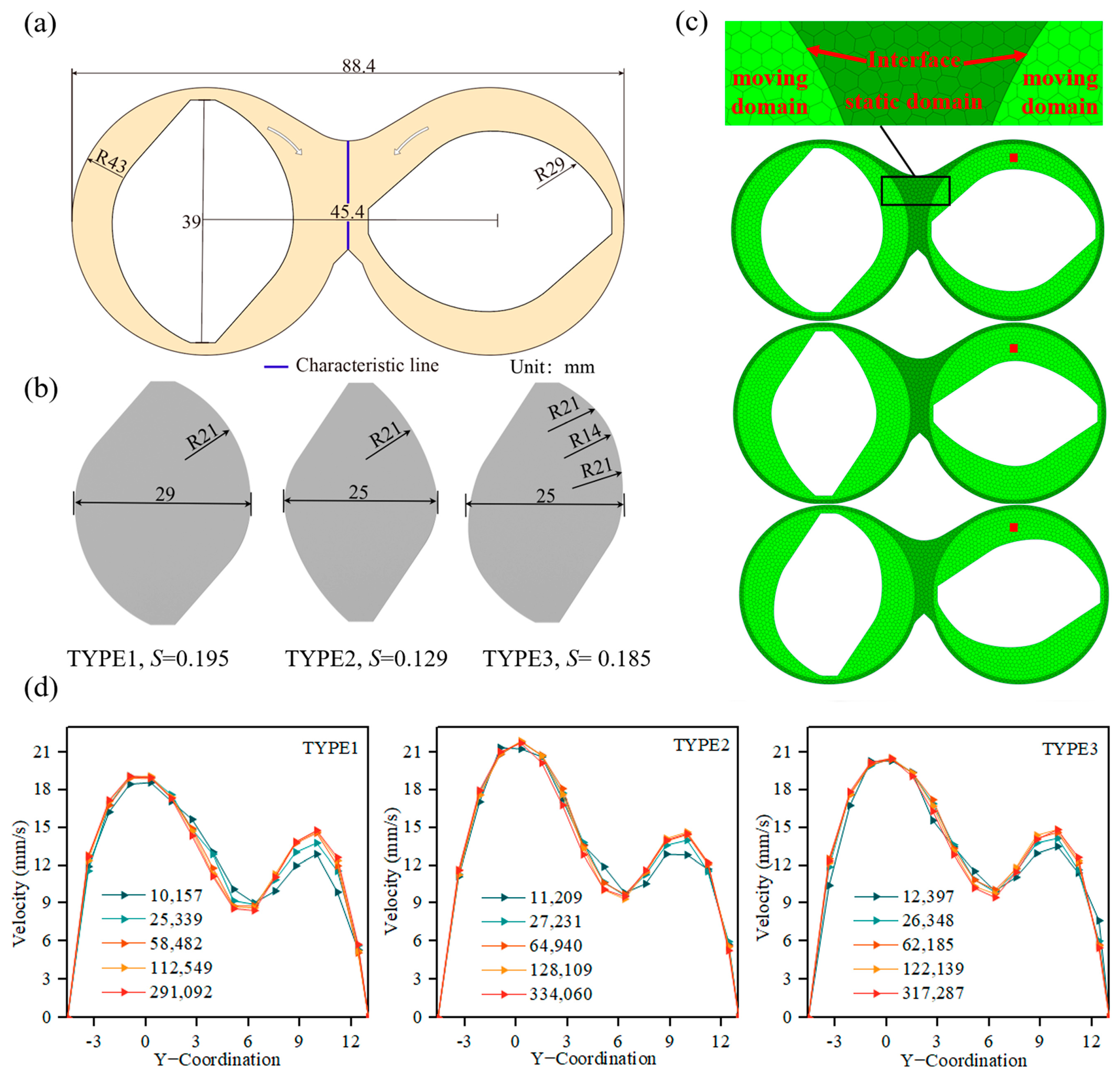
2.4. Mixing Process Simulation

The structure of batch mixer is presented in Figure 2a. Length and height of mixing chamber is 88.4 mm and 43 mm. Two rotors are phased by 90° and rotated in opposite directions. The tip between the rotor and chamber wall is 2 mm. The center distance between the left and right rotors is 45.4 mm. A characteristic line (coordinates is (0, −4.59, 0), (0, 12.84, 0)) marked with blue is selected to perform grid independence verification. The specific size and S of rotor are presented in Figure 2b. The polymer melt is LLDPE at 180 °C, and the viscosity is 576 Pa·s and assumed unchanging. The rotation speed studied in this paper is 14.35 r/min, 28.7 r/min, 43.05 r/min, 57.4 r/min and 71.75 r/min. The flow model of the melt is laminar, and AMD EPYC 7543 32-Core Processor 2.80 GHz processor (AMD, Santa Clara, CA, USA) is used. The verification of experimental equipment and simulation results is demonstrated in the Supplementary Materials.

Slide mesh is chosen because sliding interfaces are preferred for simulating rotational motion with maintaining grid consistency [32,33,34]. The meshing is obtained by using ANSYS Fluent’s polyhedral mesh, which is a great choice for reducing computation resource compared to tetrahedral and hexahedral grids. In addition, polyhedral grids can transfer data with more accurate and faster convergence [35]. The meshing result is listed in Figure 2c. In local enlarged picture, the light and dark green regions represent the moving and static domain, respectively. The agglomerate is initially settled at red square as Figure 2c presenting. The velocity on characteristic line for different grid number is demonstrated in Figure 2d. For reducing simulation time, grid number for different rotors are 58,482, 64,940 and 62,185, respectively. The cohesive force between particles is represented by bonding strength, which including normal stiffness per area, normal stress limit, tangential stiffness per area and tangential stress limit is related to a factor λ as

Table 1. The relationship between strength factor λ and bonding strength.

Normal Stiffness per Area (N/m3)	Normal Stress Limit (Pa)	Tangential Stiffness per Area (N/m3)	Tangential Stress Limit (Pa)
λ × 1010	λ × 109	λ × 1010	λ × 109

illustrating. In this paper, the value of λ is set as from 1 to 7. Other required information and parameters setting associate with the simulations are listed in

Table 2. Information and parameter setting in simulation.

Simulation Method	Parameters	Value
CFD	Melt Viscosity (Pa∙s)	576
	Melt Density (Kg/m3)	900
	Time Step	0.001
DEM	Shape	Sphere
	Diameter (mm)	0.2
	Density (Kg/m3)	2710
	Restitution coefficient	0.3
	Distance Factor	0.2
	Damping Ratio	0.1
	Adhesive Distance	0.1
	Gap Scale Factor	1.1
	Time Step	1 × 10−9
	Particle number	2120

.

3. Quantitative Evaluation of Mixing Process

3.1. Breakup Process

The characteristic dimension of the agglomerate can be quantitatively represented by gyration radius R_gy, which is defined as [36]:

$$R_{\mathit{gy}}=\sqrt{{\displaystyle \frac{1}{X}}{{\displaystyle {\sum }_{i=1}^N(r_i-r_c)}}^2}$$

(18)

$$r_c={\displaystyle \frac{1}{X}}{\displaystyle {\sum }_{i=1}^N{r}_i}$$

(19)

$r_i=(x_i,y_i,z_i)$ represents center coordinates of particle i, and r_c is assumed to be the mass center of the agglomerate. Basing on the simulation results, the coordinates for every single particle is got using an automate custom-built post-processing program, and the calculation procedure of r_c and R_gy is presented in Figure 3. The particle coordinates at the different mixing time (t) are extracted from DEM result, and the distance D_j between two particles is calculated. Then, D_j is compared with the particle diameter (D) and mean distance between particles (D_a) at t = 0, and valued as 1 or 0. After valued, D_j is stored in a logical adjacency matrix M. 1 indicates that two particles are in connect and 0 indicates no connect. The “graph” function is used to imaging the broken agglomerate from M. Then, particles’ coordinates are obtained using “conncomp” and “find” functions, and R_gy for each aggregate is calculated according to Equations (18) and (19). Then, the average value of R_gy could be obtained and marked with R_gyA.

3.2. Distributive Process

Firstly, the agglomerate is broken up, then distributed in different regions. To evaluate the distribution state, cell counting method originated from biological research [22] is used, and the ε at different t is automatically calculated according to the procedure in Figure 3. A rectangle net composed of square cell with length 2 mm is used to cover the flow domain as Figure 3 demonstrating. Length of the net is l = 90 mm, and width is of d = 44 mm. Center coordinate of the particle is used to judge the particle is in which cell. The total cell number covered the flow domain is marked with m. Owing to the difference between rotors, the m is 383, 416 and 387 for TYPE1, TYPE2 and TYPE3 rotor, respectively. After inputting the particle coordinates, the Particle number in single cell is counted by “histcounts” function and stored in a 45 × 22 matrix B. Non zero values in B are put into a matrix $N\{n_1,n_2,n_3,\dots ,n_{m-1},n_m\}$. The standard deviation of N is calculated and renamed as distribution density (ε), which is used to evaluate the distribution state.

4. Results and Discussions

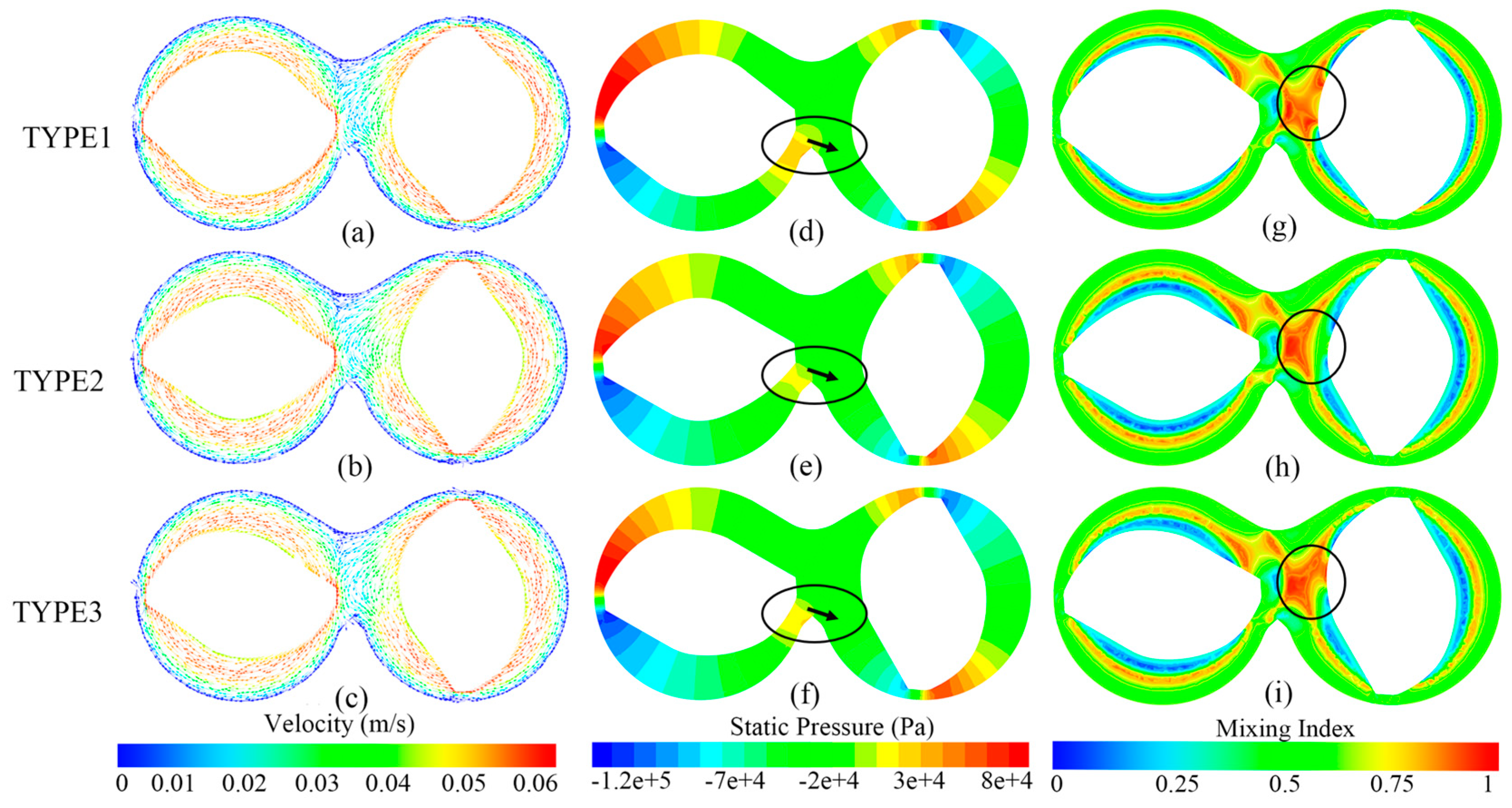
4.1. Flow Field and Mixing Process

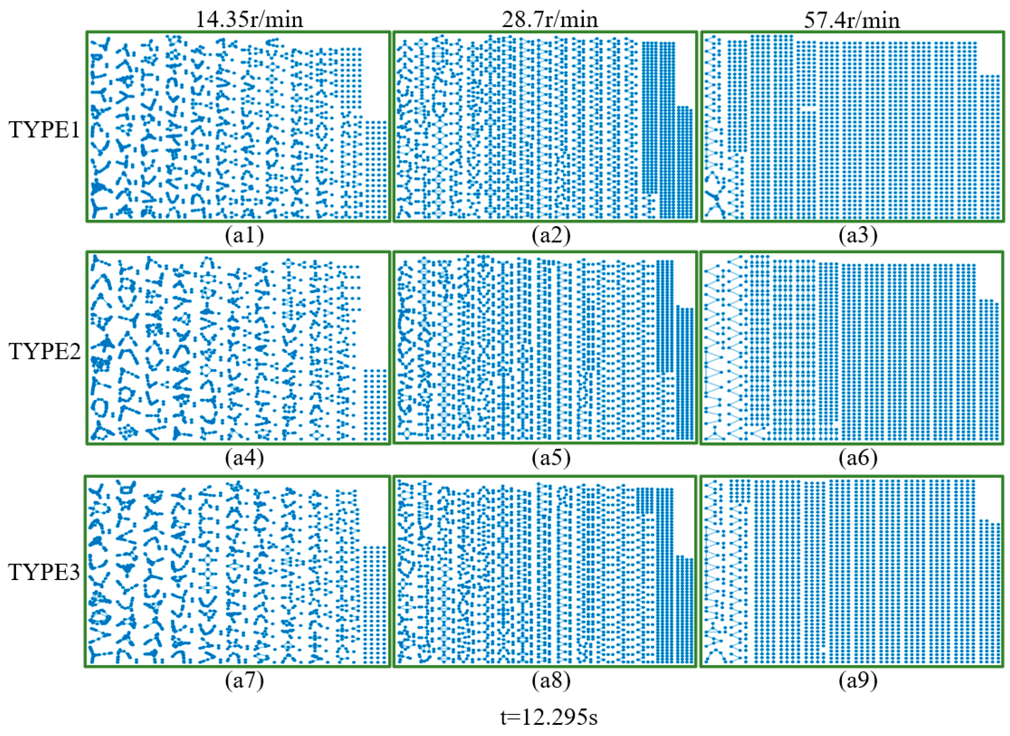
The CFD results, such as velocity vector, pressure and mixing index, could be used to characterize the flow field, and had been presented in Figure 4. The rotor rotated at a speed of 28.70 r/min and had moved 1/4 revolutions. In Figure 4a–c, velocity vector distributions for three kinds of rotor were similar, and the difference was the velocity magnitude. In the interaction window, polymer melt would be exchanged under the pushing effect originated from the right rotor. Combined with pressure cloud pictures in Figure 4d–f, the pressure near the leading face of left rotor in black circle for TYPE1 rotor was the highest, which indicating that the most polymer melt could be compressed into right chamber as black arrow indicating. More compressed polymer melt interaction window stated that the distribution could be improved. Meanwhile, higher pressure could facilitate the agglomerate breakup process. For cloud pictures of mixing index in Figure 4g–i, the rotation, shear and elongational flow were formed. The area of elongational flow in Figure 4g was much more other pictures in black circle region. It had been proved that elongational flow was more effective in promoting breakup and distribution process in mixing. So the TYPE1 rotor illustrates the best mixing ability. Basing on the discussion above, the mixing ability could be judged qualitatively by characterizing the flow field with velocity vector, pressure and mixing index. Mixing ability for three rotors was ranged as: Type1 > Type3 > Type2.

4.2. Mixing Process

By using CFD-DEM simulation method, the mixing process could be clearly illustrated. Figure 5 presented the mixing state for different rotors and rotation speeds at t = 0.955 s, t = 12.295 s and t = 20 s, and λ was 1. At the moment of t = 0.955 s and the speed of 14.35 r/min, the agglomerate shape was slightly changed, and a little part was about to leave the main body of agglomerate owing to the velocity difference of particles in Figure 5(a1) for TYPE1 rotor. At the speed of 28.7 r/min in Figure 5(a2), although shape of agglomerate had been changed, the most particles still stacked together, apart from some fast-moving particles (marked with red color). When the speed was 57.4 r/min, the agglomerate had been stretched into rod shape in region near the leading face, and the particles at rotor tip and back face were compressed to form a long line. The rod or line shape composed of particles formed at higher rotation speed proved that improving the rotation speed was very effective for facilitating the breakup process. In another word, improving speed would make the agglomerate experiencing the breakup process faster. The faster broken of the agglomerate in mixing, the more beneficial the distribution process. At the moment of t = 12.295 s in Figure 5(b1–b3), the distribution state of broken agglomerate was improved by enhancing the rotation speed, which would be further proved in Figure 5(c1–c3). The mixing state for TYPE2 and TYPE3 rotor in Figure 5 will present similar process. Thus, it could be concluded that larger rotation speed could benefit the breakup and distribution process.

For the rotors with different S, obvious distinctions for mixing process could also be observed. When the speed was 14.35 r/min, the shape and broken state of the agglomerate were almost the same in Figure 5(a1,a4,a7), so mixing state difference was not so clearly at t = 0.955 s. At t= 12.295 s, the particles formed the line or rod shape in Figure 5(b1) for TYPE1 rotor. In Figure 5(b4) for TYPE2 rotor, the lines or rods formed by particles were thicker than that in Figure 5(b1). As for the mixing process of TYPE3 rotor, the particles also formed line or rod shape, which were thinner than that for TYPE2 rotor. The breakup state was further improved when mixing time reaching 20 s. When rotation speed improved to 28.7 r/min in Figure 5(a2,a5,a8), the shape of agglomerate had been greatly changed for three rotors. In Figure 5(a2), the agglomerate had been broken, and the broken parts presented stretching deformation. The breakup process was not observed for TYPE2 and TYPE3 rotor, but the agglomerate was more stretched and about to be broken in Figure 5(a8) than that in Figure 5(a5). In Figure 5(a3,a6,a9), the agglomerates had been stretched into a rod or line shape, and the rod thickness near the leading face region for TYPE1 rotor was much thinner than that in TYPE2 and TYPE3 rotor. Thus, the breakup ability for three rotors at the initial mixing stage was found to be in the order TYPE1 > TYPE3 > TYPE2, which was consistent with the S value of rotors. As for the distribution process, although some obvious distinctions could be observed when agglomerate was continuously broken into small pieces, the mixing process for different rotors were still hard to be clearly or accurately compared from the picture results as Figure 5(b1–b9,c1–c9) presenting, especially in Figure 5(c3,c6,c9). Meanwhile, the breakup process was also difficult to be observed and compared when agglomerate had been broken into small pieces. So, further processing of the picture results was needed.

4.3. Evaluation and Kinematics Analyzation

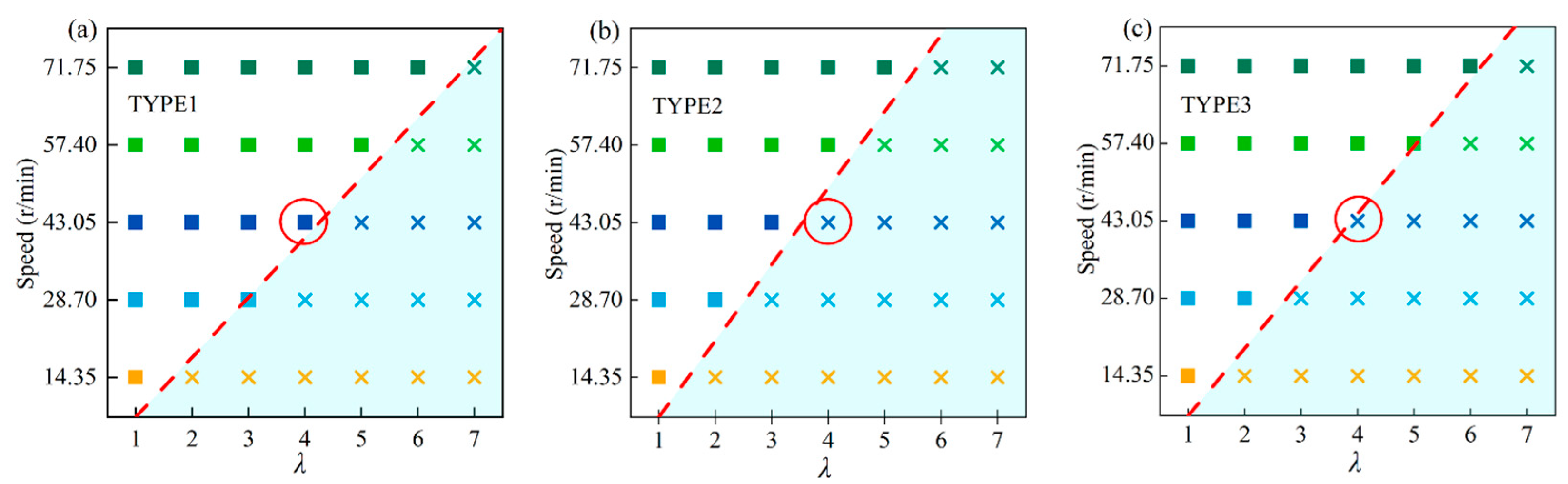
To evaluate the mixing process, the R_gyA and ε were automatically obtained according to the procedure in Figure 3. The broken agglomerate presented interesting shape after the simulation data was processed with “graph” function, and the part results were presented in Figure 6(a1–a9). At the moment of t = 12.295 s, the agglomerate had been broken into V-, U- or Y-shape as Figure 6(a1,a4,a7) showing. Besides, some particles had achieved mono-dispersion. The V-, U- or Y-shape formed by particles indicating that the broken agglomerate would experience stretching and folding during the mixing process, which further proved that the chaotic mixing was the major reason for the breakup and the distribution of agglomerate. Meanwhile, the automatic post-processing method established in this study was found to be reliable and accurate. A comparison of the results in Figure 5b with those presented in Figure 6 revealed that rotor with higher rotation speed and larger S would produce a greater number of mono-dispersed particles and smaller V-, U-, or Y-shape aggregates.

For evaluating the breakup process, the R_gyA/r was calculated because R_gyA/r = 1 meant that the agglomerate was broken into mono-dispersed particles, which was the most desired dispersive mixing state. Overall, curves of R_gyA/r versus t varied similarly for rotors with different S and rotation speed as illustrated in Figure 7a–c. However, a notable decline in the value of R_gyA/r was observed following an increase. The sharp decline in R_gyA/r signified the disintegration of substantial agglomerates or aggregates, whereas the elevated value reflected the deformation. In light of the deliberations presented in Section 4.2, it can be postulated that large agglomerates or aggregates would undergo a process of stretching. Furthermore, the rise and subsequent decline of R_gyA/r were observed exclusively prior to t = 4 s (named as critical time) in Figure 7a. It was also noted that the R_gyA/r would decrease monotonically with an increase in t. After the critical time, the breakup process became more and more frequently and R_gyA/r changed less and less, eventually returning to a stable value. The same phenomenon was also observed in Figure 7b,c, and the only difference was the critical time, which was 2 s and 0.3 s for 28.7 r/min and 57.4 r/min, respectively. In comparison to the other two rotors, the TYPE1 rotor with the largest S experienced the breakup process at an earlier time and reached the lowest R_gyA/r value. In Figure 7c, the value of R_gyA/r was very close to 1, indicating that the mono-dispersion was almost realized for TYPE1 rotor at a rotational speed of 57.4 r/min and a time of 10 s. Although the agglomerate showed the most pronounced stretching deformation at the initial mixing stage for the TYPE2 rotor with the smallest S, the R_gyA/r value was the highest at t = 20 s. Above all, the R_gyA/r value could quantitatively assess the breakup state of agglomerate, while the curve of R_gyA/r versus t could help to analyze the breakup kinematics.

In DEM simulation, the particle number was 2120, and the number of cells covered the flow domain was 383, 416 and 387 for TYPE1, TYPE2 and TYPE3 rotor, respectively. As illustrated in Figure 7d–f, the value of ε exhibited a continuous decrease with an increase in t, which suggested that the broken agglomerate was distributed. The value of ε for the TYPE1 rotor demonstrated the lowest value at different rotation speeds, indicating that the TYPE1 rotor exhibited the most optimal distribution ability. In Figure 7f, the value of ε was almost kept unchanged since t = 8 s, t = 12 s and t = 14 s for TYPE1, TYPE2 and TYPE3 rotor, respectively. The findings indicated that the particles could not be further distributed after a certain mixing time, because it had reached the final distribution state. Additionally, the TYPE1 rotor was observed to reach the final distribution state more rapidly than the other two rotors. Thus, the distribution ability for three rotors was found to be in the order TYPE1 > TYPE3 > TYPE2, which was also consistent with the S value of rotors.

The R_gyA/r and ε versus t curves for TYPE1 rotor were plotted in Figure 8 for the purpose of considering the influence of bonding strength (related to λ) between particles on the breakup and distribution process. A large λ meant that the agglomerate was difficult to be broken. At the initial stage of mixing, agglomerate with λ = 1 would be broken firstly as shown in Figure 8, and the R_gyA/r was the smallest at t = 20 s. As λ was increased to 3, more time was needed to realize the first breakup, and the R_gyA/r would become larger than λ = 1 at t = 20 s. Meanwhile, the value of ε was increased with λ improved from 1 to 3, suggesting that the distribution became progressively worse. In a word, a larger λ would hinder the breakup and distribution process.

4.4. Breakup-Line

Breakup of the agglomerate was a prerequisite for mixing process, because only the agglomerate was broken up into aggregates, pieces or mono-dispersed particles, thereby achieving the distribution. In this paper, the influence of the rotor configuration and rotation speed on breakup process had been discussed, and the agglomerate could be broken when bonding strength λ = 1. To investigate the agglomerate breakup situation at higher λ (i.e., stronger bonding between the particles), the mixing processes were simulated at different rotation speeds and λ. In the event that the agglomerate was found to be broken at a given rotation speed and λ, a square was plotted in a coordinate system comprising of rotational speed and λ. Otherwise, a cross was plotted. Consequently, the plotting results were presented in Figure 9 for different rotors. The red dotted line was the “breakup line”, which was derived through fitting the boundary between agglomerate breakup and non-breakup. The agglomerate could be broken if the combination of rotation speed and λ was above the “breakup line”, otherwise the agglomerate was not broken. As shown in Figure 9, the agglomerate became more and more difficult to be broken with increasing λ when the rotation speed was fixed. On the other hand, when λ was fixed, improving the rotational speed would favor the agglomerate breakup.

Moreover, the slope of the “breakup line” for TYPE1 rotor was observed to be the minimum in Figure 9a, yet the breakup area in the coordinate system was the largest, which suggested that the TYPE1 rotor exhibited the strongest breakup ability. The slope of “breakup line” for TYPE1, TYPE2 and TYPE3 rotor were 11.03, 14.07 and 12.38, respectively. The data indicated that the order of breakup ability for three rotors was TYPE1 > TYPE3 > TYPE2. This finding was consistent with the discussions presented in the preceding sections. Thus, it could be proposed that the slope of “breakup line” might be used as a parameter for evaluating the breakup ability of different rotors.

5. Conclusions

This paper presented a simulation work for the purpose of evaluating the breakup and distribution process of an agglomerate in batch mixer. The simulation work is performed by using CFD-DEM coupling method, and a bonding model is introduced to describe the cohesive force within the agglomerate. An automatic post-processing method is proposed to calculate the R_gyA and ε from the simulation results.

The agglomerate is broken under a series of stretching and folding operations, resulting in the formation of V-, U-, or Y-shaped aggregates, suggesting that chaotic mixing plays a pivotal role in the functioning of the batch mixer. With the agglomerate is broken, R_gyA/r exhibited a decrease over mixing time, and a notable decline in the value of R_gyA/r is observed following an increase prior to critical time. The increase of R_gyA/r stated that the aggregates or pieces would undergo a stretching deformation. After the critical time, the R_gyA/r is continuously decreased. The broken agglomerate is constantly distributed, because the ε became smaller and smaller with mixing time increasing. The rotor configuration is characterized by pressurization coefficient (S). And, rotor with large S and rotation speed would intensify and facilitate the breakup and distribution process in mixing, while strong bonding strength would hinder the breakup and distribution process. A “breakup line” is established by fitting the boundary between breakup and non-breakup of the agglomerate in a coordinate system composed of rotation speed and bonding strength. The agglomerate could be broken if the combination of rotation speed and bonding strength is above the “breakup line”, otherwise the agglomerate is not broken. Large slope meant strong breakup ability, so the slope of “breakup line” could be used as a parameter for evaluating the breakup ability of different rotors. The simulation and post-processing method in this paper could be used to quantitatively evaluate the breakup and distribution process for other mixing process, and give a through kinematics analyzation.

References

1. Boudenne, A.; Ibos, L.; Fois, M.; Majesté, J.; Géhin, E. Electrical and thermal behavior of polypropylene filled with copper particles. Compos. Part A Appl. Sci. Manuf. 2005, 36, 1545–1554. [Google Scholar] [CrossRef]
2. Hernandez, F.H.; Rangel, R.H. Breakup of drops in simple shear flows with high-confinement geometry. Comput. Fluids 2017, 146, 23–41. [Google Scholar] [CrossRef]
3. Avolio, R.; Castaldo, R.; Avella, M.; Cocca, M.; Gentile, G.; Fiori, S.; Errico, M.E. PLA-based plasticized nanocomposites: Effect of polymer/plasticizer/filler interactions on the time evolution of properties. Compos. Part B Eng. 2018, 152, 267–274. [Google Scholar] [CrossRef]
4. Azoug, A.; Nevière, R.; Pradeilles-Duval, R.; Constantinescu, A. Influence of crosslinking and plasticizing on the viscoelasticity of highly filled elastomers. J. Appl. Polym. Sci. 2014, 131, 40392. [Google Scholar] [CrossRef]
5. Gopalkrishnan, P.; Manas-Zloczower, I.; Feke, D. Investigating dispersion mechanisms in partially infiltrated agglomerates: Interstitial fluid effects. Powder Technol. 2005, 156, 111–119. [Google Scholar] [CrossRef]
6. Fanelli, M.; Feke, D.L.; Manas-Zloczower, I. Prediction of the dispersion of particle clusters in the nano-scale—Part II, unsteady shearing responses. Chem. Eng. Sci. 2006, 61, 4944–4956. [Google Scholar] [CrossRef]
7. Pomchaitaward, C.; Manas-Zloczower, I.; Feke, D. Investigation of the dispersion of carbon black agglomerates of various sizes in simple-shear flows. Chem. Eng. Sci. 2003, 58, 1859–1865. [Google Scholar] [CrossRef]
8. Potente, H.; Kretschmer, K.; Flecke, J. A physical-mathematical model for the dispersion process in continuous mixers. Polym. Eng. Sci. 2004, 42, 19–32. [Google Scholar] [CrossRef]
9. Hosseini, M.S.; Nazockdast, H.; Anderson, P.D.; Meijer, H.E.H. Simulation of Agglomerate Dispersion in Cubic Cavity Flow. Macromol. Theory Simul. 2009, 18, 201–208. [Google Scholar] [CrossRef]
10. Jiang, G.; Huang, H. Melt-compounding of PP/clay nanocomposite and relationship between its microstructure and shear strain in the flow field based on rheological analysis. Polym. Eng. Sci. 2011, 51, 2345–2352. [Google Scholar] [CrossRef]
11. Wéry, F.; Vandewalle, L.A.; Marin, G.B.; Heynderickx, G.J.; Van Geem, K.M. Hydrodynamic CFD-DEM model validation in a gas–solid vortex unit. Chem. Eng. J. 2023, 455, 140529. [Google Scholar] [CrossRef]
12. Zhou, M.; Wang, S.; Kuang, S.; Luo, K.; Fan, J.; Yu, A. CFD-DEM modelling of hydraulic conveying of solid particles in a vertical pipe. Powder Technol. 2019, 354, 893–905. [Google Scholar] [CrossRef]
13. Esgandari, B.; Golshan, S.; Zarghami, R.; Sotudeh-Gharebagh, R.; Chaouki, J. CFD-DEM analysis of the spouted fluidized bed with non-spherical particles. Can. J. Chem. Eng. 2021, 99, 2303–2319. [Google Scholar] [CrossRef]
14. Frungieri, G.; Boccardo, G.; Buffo, A.; Marchisio, D.; Karimi-Varzaneh, H.A.; Vanni, M. A CFD-DEM approach to study the breakup of fractal agglomerates in an internal mixer. Can. J. Chem. Eng. 2020, 98, 1880–1892. [Google Scholar] [CrossRef]
15. Manas-Zloczower, I.; Cheng, H.F. Influence of design on mixing efficiency in the kneading disc region of co-rotating twin screw extruders. J. Reinf. Plast Compos. 1998, 17, 1076–1086. [Google Scholar] [CrossRef]
16. Connelly, R.K.; Kokini, J.L. Examination of the mixing ability of single and twin screw mixers using 2D finite element method simulation with particle tracking. J. Food Eng. 2007, 79, 956–969. [Google Scholar] [CrossRef]
17. Mewes, D. The kinematics of mixing: Stretching, chaos, and transport. AlChE J. 1990, 38, 316–317. [Google Scholar]
18. Danckwerts PVJIICE. The definition and measurement of some characteristics of mixtures. Appl. Sci. Res. 1981, 3, 268–287. [Google Scholar]
19. Nakayama, Y.; Kajiwara, T.; Masaki, T. Strain mode of general flow: Characterization and implications for flow pattern structures. AIChE J. 2016, 62, 2563–2569. [Google Scholar] [CrossRef]
20. Ferrás, L.L.; Fernandes, C.; Semyonov, D.; Nóbrega, J.M.; Covas, J.A. Dispersion of Graphite Nanoplates in Polypropylene by Melt Mixing: The Effects of Hydrodynamic Stresses and Residence Time. Polymers 2021, 13, 102. [Google Scholar] [CrossRef]
21. Berzin, F.; Vergnes, B.; Lafleur, P.G.; Grmela, M. A theoretical approach to solid filler dispersion in a twin-screw extruder. Polym. Eng. Sci. 2002, 42, 473–481. [Google Scholar] [CrossRef]
22. Labib, M.; Philpott, D.N.; Wang, Z.; Nemr, C.; Chen, J.B.; Sargent, E.H.; Kelley, S.O. Magnetic Ranking Cytometry: Profiling Rare Cells at the Single-Cell Level. Accounts Chem. Res. 2020, 53, 1445–1457. [Google Scholar] [CrossRef] [PubMed]
23. Frungieri, G.; Boccardo, G.; Buffo, A.; Karimi–Varzaneh, H.A.; Vanni, M. CFD-DEM characterization and population balance modelling of a dispersive mixing process. Chem. Eng. Sci. 2022, 260, 117859. [Google Scholar] [CrossRef]
24. Potyondy, D.O.; Cundall, P.A. A bonded-particle model for rock. Int. J. Rock Mech. Min. Sci. 2004, 41, 1329–1364. [Google Scholar] [CrossRef]
25. Cho, N.; Martin, C.D.; Sego, D.C. A clumped particle model for rock. Int. J. Rock Mech. Min. Sci. 2007, 44, 997–1010. [Google Scholar] [CrossRef]
26. Guo, Y.; Wassgren, C.; Curtis, J.S.; Xu, D. A bonded sphero-cylinder model for the discrete element simulation of elasto-plastic fibers. Chem. Eng. Sci. 2018, 175, 118–129. [Google Scholar] [CrossRef]
27. Vallejos, J.A.; Salinas, J.M.; Delonca, A.; Ivars, D.M. Calibration and Verification of Two Bonded-Particle Models for Simulation of Intact Rock Behavior. Int. J. Géoméch. 2017, 17, 06016030. [Google Scholar] [CrossRef]
28. Hare, C.; Ghadiri, M.; Guillard, N.; Bosworth, T.; Egan, G. Analysis of milling of dry compacted ribbons by distinct element method. Chem. Eng. Sci. 2016, 149, 204–214. [Google Scholar] [CrossRef]
29. Ge, R.; Ghadiri, M.; Bonakdar, T.; Zheng, Q.; Zhou, Z.; Larson, I.; Hapgood, K. Deformation of 3D printed agglomerates: Multiscale experimental tests and DEM simulation. Chem. Eng. Sci. 2020, 217, 115526. [Google Scholar] [CrossRef]
30. Giménez, C.S.; Finke, B.; Nowak, C.; Schilde, C.; Kwade, A. Structural and mechanical characterization of lithium-ion battery electrodes via DEM simulations. Adv. Powder Technol. 2018, 29, 2312–2321. [Google Scholar] [CrossRef]
31. Di Felice, R. The voidage function for fluid-particle interaction systems. Int. J. Multiph. Flow 2003, 20, 153–159. [Google Scholar] [CrossRef]
32. Cao, Y.; Liu, A.; Yu, X.; Liu, Z.; Tang, X.; Wang, S. Experimental tests and CFD simulations of a horizontal wave flow turbine under the joint waves and currents. Ocean Eng. 2021, 237, 109480. [Google Scholar] [CrossRef]
33. Greaves, D. A quadtree adaptive method for simulating fluid flows with moving interfaces. J. Comput. Phys. 2004, 194, 35–56. [Google Scholar] [CrossRef]
34. Brown, S.; Ransley, E.; Greaves, D. Developing a coupled turbine thrust methodology for floating tidal stream concepts: Verification under prescribed motion. Renew. Energy 2020, 147, 529–540. [Google Scholar] [CrossRef]
35. Chen, H.; Zhou, X.; Feng, Z.; Cao, S.-J. Application of polyhedral meshing strategy in indoor environment simulation: Model accuracy and computing time. Indoor Built Environ. 2022, 31, 719–731. [Google Scholar] [CrossRef]
36. Dizaji, F.F.; Marshall, J.S.; Grant, J.R. Collision and breakup of fractal particle agglomerates in a shear flow. J. Fluid Mech. 2019, 862, 592–623. [Google Scholar] [CrossRef]
Figure 1. Description for the adhesive contact model.
Processes 12 02840 g001
Figure 2. The configuration and meshing for batch mixer: (a) flow domain; (b) rotor; (c) slide meshing; (d) grid independence verification, rotation speed is 28.7 r/min.
Processes 12 02840 g002
Figure 3. Calculating procedure schemes for RgyA and ε.
Processes 12 02840 g003
Figure 4. Flow characterize of TYPE1, TYPE2 and TYPE3 rotor: (ac) velocity vector pictures; (df) pressure cloud pictures; (gi) mixing index cloud picture. Rotor rotational speed was 28.70 r/min, respectively, and rotors had rotated 1/4 revolutions.
Processes 12 02840 g004
Figure 5. Mixing state of different rotors at (a1a9) t = 0.955 s, (b1b9) t = 12.295 s and (c1c9) t = 20 s; the rotation speeds were 14.35 r/min, 28.7 r/min and 57.4 r/min, respectively; λ = 1.
Processes 12 02840 g005
Figure 6. The morphology of broken agglomerate after processed with “graph” function at the moment of t = 12.295 s when λ = 1.
Processes 12 02840 g006
Figure 7. Curves for the RgyA/r (r was the particle radius) and ε changing with mixing time for different rotors and rotation speeds, and λ = 1.
Processes 12 02840 g007
Figure 8. RgyA/r and ε versus t curves for TYPE1 rotor under different λ, and the rotation speed was 28.7 r/min.
Processes 12 02840 g008
Figure 9. Established “breakup-line” for different rotors: (a) type1 rotor; (b) type2 rotor; (c) type3 rotor.
Processes 12 02840 g009