The Integration of Image Intensity and Texture for the Estimation of Particle Mass in Sorting Processes

Abstract

Although mass is one of the most relevant process variables, industries may lack an inline monitoring of mass, which has a high cost in some cases. Due to their availability in sorting processes, cameras have potential as a low-cost alternative for the estimation of mass in recycling applications. Nevertheless, further research is needed to transform image information into mass. This work tackles this challenge by proposing a novel method of converting image information into mass of particles, complementing size measures with intensity and texture features extracted from the whole picture. Models were adjusted, employing machine learning techniques, using an industrial waste sample of post-consumer plastic film. The visual properties showed a dependency on mass labels, and the models achieved an error of 9 g for subsamples between 2 and 82 g. The analysis and validation of this image processing method provide a new alternative for the estimation of particle mass.

1. Introduction

1.1. Monitoring of Mass Flow for Recycling Processes

The monitoring of mass is key for the control of multiple industries, such as mining [1,2], polymer manufacturing [3], pharmaceutics [4], and recycling [5]. The measurement of mass also enables the speed of belt conveyors to be controlled, which can reduce their energy consumption for loads under the nominal regime [6].

In waste management, mass is a key characteristic of the material flow, and it is determined to conduct techno-economic [7] and environmental [8,9] analyses. Weight is also essential to evaluating sorting processes via the variables of recovery, yield, and purity [10]. Moreover, variations in material load are one of the main causes of suboptimal recycling rates, and flow control can enhance the operation of sorting systems [11]. An increase in occupation density (throughput rate) may result in an increase in product quantity but an exponential decrease in recovery and yield [12]. Assuming that the ejected fraction of a sorting process can be sold at different prices depending on its purity, the throughput rate can be adjusted to maximize profit [12]. In sum, an increase in mass measurement accuracy may improve process assessments and sorting performance and also increase economic gains.

The technologies used for mass flow sensors comprise scales (based on load cells or radiation), plates (baffle or impact), and flow slides [13]. Regardless of the chosen alternative, all of them have little practical application for bulk materials with low density, such as plastic foils. Furthermore, their cost may be a limiting factor according to their application, as in the case of waste sorting and recycling facilities. The implementation of low-cost sensors for material flow characterization has future research potential in waste treatment [14].

In addition to measurement, mass flow can also be estimated based on other variables. Volume flow sensors can be used to compute mass flow at a lower cost than mass flow sensors [13]. However, the volume can change due to variations in bulk density [14]. Thus, the method used to compute mass from volume may be complex, and it requires research before being applied in material flow characterization.

Several technologies can be employed to measure volume, such as laser, infrared, ultrasound, and radar (microwaves) technologies [13]. Furthermore, volume can be monitored with three-dimensional (3D) and two-dimensional (2D) cameras. Comparing lasers and 3D state-of-the-art cameras, lasers may be preferred due to their lower cost [14]. Nevertheless, waste treatment plants may use cameras for sorting tasks, while they lack lasers. Thus, the use of these cameras for the measurement of volume flow could be cheaper than the installation of a laser.

1.2. Volume Measurement Using Cameras

Laser 3D cameras have been employed to sort waste streams based on volume measurements. Mattone et al. [15] applied this method for packaging waste, while Koyanaka and Kobayashi [16] focused on wrought and cast aluminum and magnesium. Other works have enhanced the method used to measure volume with 3D cameras. In the work of Qiao et al. [17], a system with two stereo 3D cameras was developed to monitor the upper and lower sides of a belt conveyor during the transport of three reference items and coal bulks. Volume was measured with an error lower than 5%, and bias due to belt deformation was reduced, avoiding calibrations without load. Xu et al. [18] proposed a different system based on a stereo 3D camera, a speed sensor, the radio frequency identification of belt segments, and the continuous estimation of bulk density. This solution was tested for bulks of fine sand and coal with different particle sizes, with a maximum error of 2%. The identification of belt segments decreased the errors of the speed sensor, and bulk density was computed based on the porosity measured by the camera.

Volume can be also computed using 2D cameras, using several cameras capturing images simultaneously [19], using a single camera whose relative position to the scene is changed [20], or using a single image [21]. Although 2D images require additional processing to provide volume measurements, their use in waste management sorting tasks is more widespread than 3D cameras. For example, in the 198 publications reviewed by Kroell et al. [14], the task of material identification was developed in 92% of cases using 2D cameras (visible, infrared, hyperspectral, and thermal technologies), while 3D cameras only accounted for 3%. The measurement of volume flow with 2D cameras could attract more interest due to their greater availability in waste facilities.

Among the different ways of measuring volume with 2D cameras, the simplest one employs a single image (monocular vision) to recover 3D information. To tackle the lack of depth information, prior information and assumptions about the scene are used to describe the volume geometry. For example, Chen et al. [21] used this approach to estimate the volume of construction and demolition waste inside the buckets of trucks. First, the truck and its loaded waste types were segmented. Next, the camera was calibrated based on a previous work [22], defining a global coordinate system. The bucket dimensions were computed by selecting their boundaries using four lines, and the volume of each waste type was calculated based on each image and the measures of eight range finders. As a result, the vision algorithm estimated waste volume with an average error of 17%.

1.3. Application of Cameras for Mass Estimation

Despite the technological readiness of digital cameras, their application in mass estimation has rarely been studied. Some works used 2D images [1,3,4], 3D point clouds [2], or both methods [5]. Mass was modeled employing only image variables [3,4] or including additional information, i.e., density [1], the average weight of size classes [2], or material information [5]. Studies on plastic manufacturing [3] and the pharmaceutical industry [4] focused on the mass range of 0–1 g, achieving relative errors of 1–4%. By contrast, applications for mining studied particle weights of up to 2 kg, with relative errors of 6% [1,2]. This performance was achieved in the monitoring of a single material, while a multi-material model for the recycling of packages reached a relative error of 24% [5]. In any case, all of these studies segmented particles in the images and extracted area and/or volume features from them.

1.4. Aim and Conclusions of the Study

This study proposes a novel image-based method for the research field of mass estimation. The procedure implements new image characteristics to estimate the total mass of the elements captured in the image. Features are extracted to characterize the intensity and texture in the whole image, together with the total area of the particles captured. Models are adjusted using machine learning techniques, evaluating three algorithms (linear, support vector machines, and multilayer perceptron).

The procedure uses a 2D camera to study a low-cost alternative of mass estimation for sorting processes, which is another research gap of the state of the art. In multiple cases, facilities for waste treatment already have this technology, which would avoid the commissioning of additional sensors to monitor mass flow.

Apart from the two previous research gaps, this work also tackles the challenge of mass monitoring of low-density materials. With that purpose, a sample of post-consumer plastic film was collected from an industrial municipal solid waste (MSW) treatment plant.

The present work validates the feasibility of the novel method of visual mass estimation. Intensity and texture features had a linear relationship with the mass labels of the images, and the models achieved an error of 9 g for subsamples between 2 and 82 g. The model performance matched previous values for lightweight packaging, validating the new procedure and setting the stage for further studies of mass modeling using intensity and texture features.

2. Materials and Methods

2.1. Industrial Waste Sample and Laboratory Test Equipment

A plastic waste sample was collected from the complex for the treatment of urban waste of Zaragoza (CTRUZ), an industrial facility dedicated to MSW processing. This plant is located in Spain and serves more than 750,000 citizens, with a processing capacity of more than 250 thousand metric tons per year of MSW and up to fifteen thousand metric tons per year of sorted light packaging waste. The CTRUZ consists of two material recovery facilities: one employed for light packaging that was collected selectively and the other for mixed MSW. In the second case, ballistic separators provide a 2D (flat and light) fraction, from which post-consumer plastic film is recovered by manual sorting. This complex includes the URBASER pilot pretreatment line (Zaragoza, Spain), which cleans and densifies the post-consumer plastic film in preparation for chemical recycling via pyrolysis. The pretreatment line has an input capacity of 400 kg/h and is fed by bales (Figure 1), whose composition is shown in

Table 1. Composition of bales recovered from post-consumer plastic film.

Material	Weight Proportion (%)
LDPE	84.20–93.50
HDPE	0.02–0.09
PP	0.17–0.38
PS	0.07–0.18
PET	0.08–0.83
PVC	0.00
Other plastics	0.30–0.80
Organic matter	1.00–2.11
Paper/cardboard	2.15–12.7
Beverage carton	0.03–0.15
Metal	0.23–0.56
Other materials	1.06–1.61

. A waste sample was collected at the start of the pretreatment line after the shredding process, obtaining one kilogram of waste particles between 10 and 15 cm, with an approximate volume of 60 L.

The laboratory setup for image acquisition is summarized in Figure 2. Waste particles were placed on a surface of 40 × 45 cm illuminated by LED lightning (ABSOLUTE SERIES 6500 K), distributed by Waveform Lighting LLC (Vancouver, WA, USA). Similar configurations were used for material characterization in previous works, without requiring a running conveyor belt [1,23,24]. A scale was used to measure mass (0.01 g accuracy), and images were acquired with an AP-1600T-PGE camera of 1.6 megapixels (JAI Ltd., Copenhagen, Denmark) placed on top of the surface as in sorting applications. This camera captures light emissions in the visible-color range, which is also a predominant alternative for material classification, together with near-infrared wavelengths [14].

2.2. Waste Characterization and Image Processing

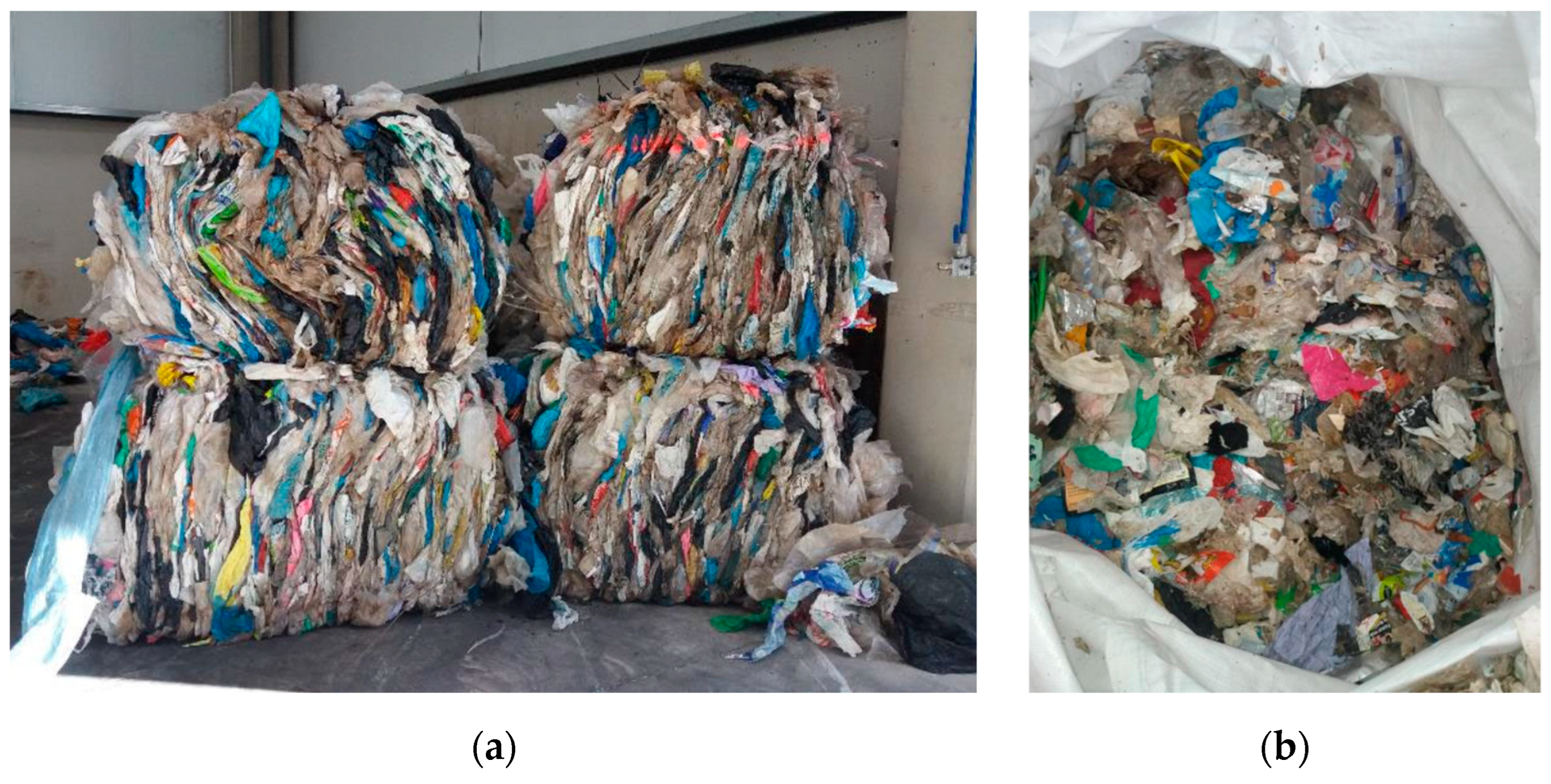
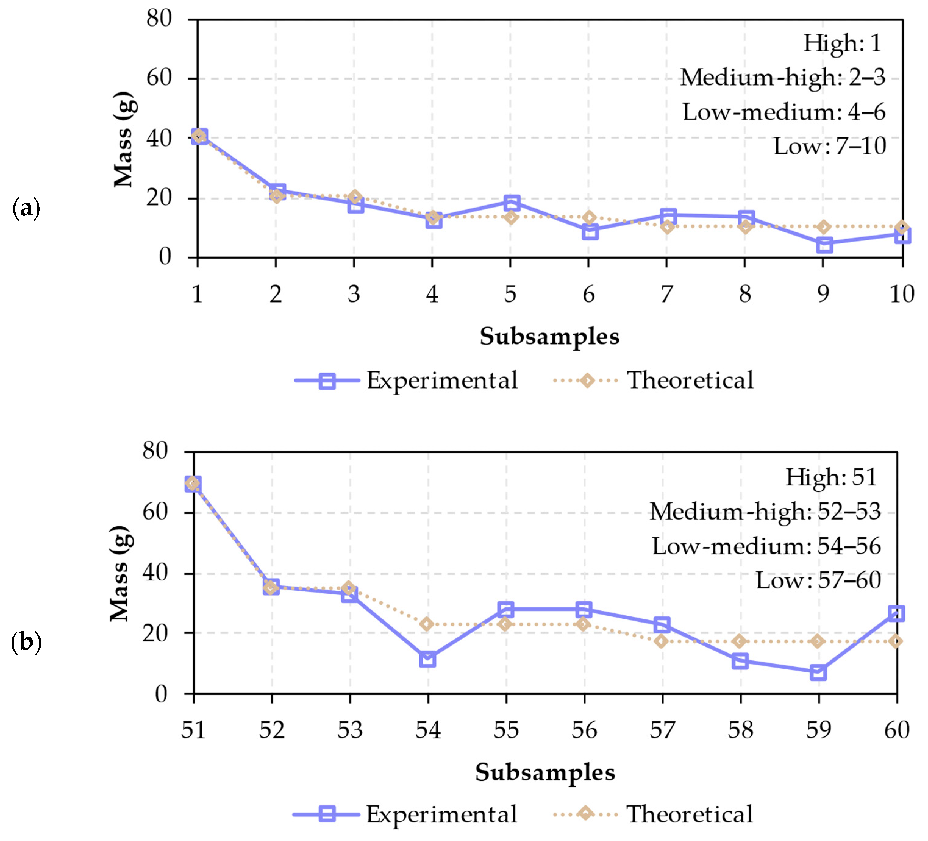
The waste sample was divided into 21 groups of different particles. Each group was defined to cover most of the inspected area, representing a high cover level. Waste fragments were presented as a single monolayer, without overlapping each other, reproducing the conditions of material flows during sorting operations [14]. On average, eight particles were used to reproduce the high load class.

To study medium-high, low-medium, and low cover levels, each group of particles was divided into two, three, and four monolayer subgroups, respectively. As an example,

Table 2. Example of particle distribution between cover levels considering a group of twelve particles with equal mass.

Cover Level	Subsamples	Waste Particles per Subsample	Load Ratio per Subsample	Relative Difference of Load Ratio (%) Between Cover Levels
High	1	12	1.00	-
Medium-high	2	6	0.50	50
Low-medium	3	4	0.33	34
Low	4	3	0.25	24

considers a group of twelve fragments with equal mass, characterizing different properties for each cover level.

The subgroups for the same load class were manually defined, aiming to reduce mass differences between them. Each particle group provided ten subgroups with different waste particles and cover levels, resulting in a total of 210 subsamples. Similar volumes of data points were used in other studies [15,25].

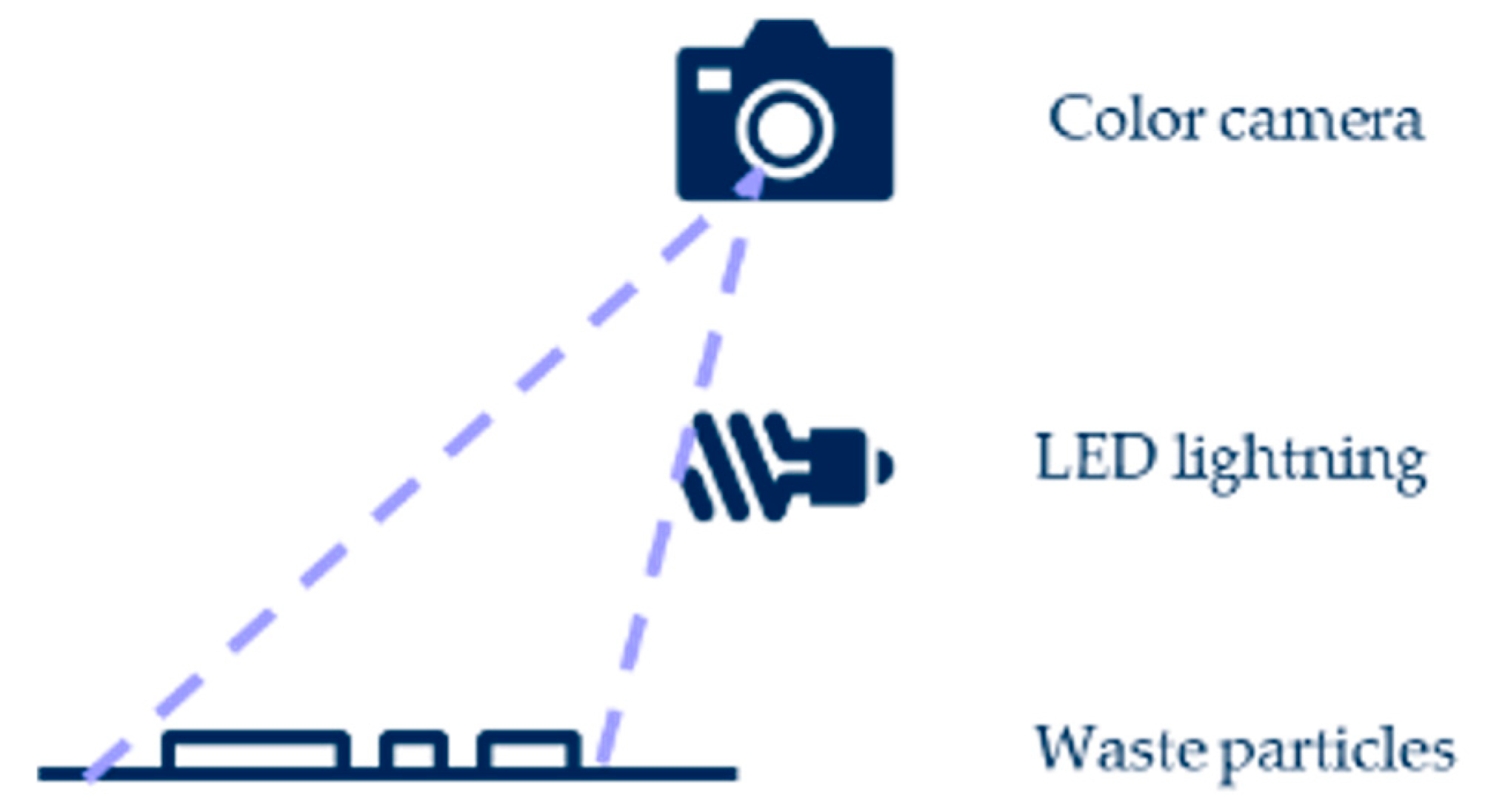
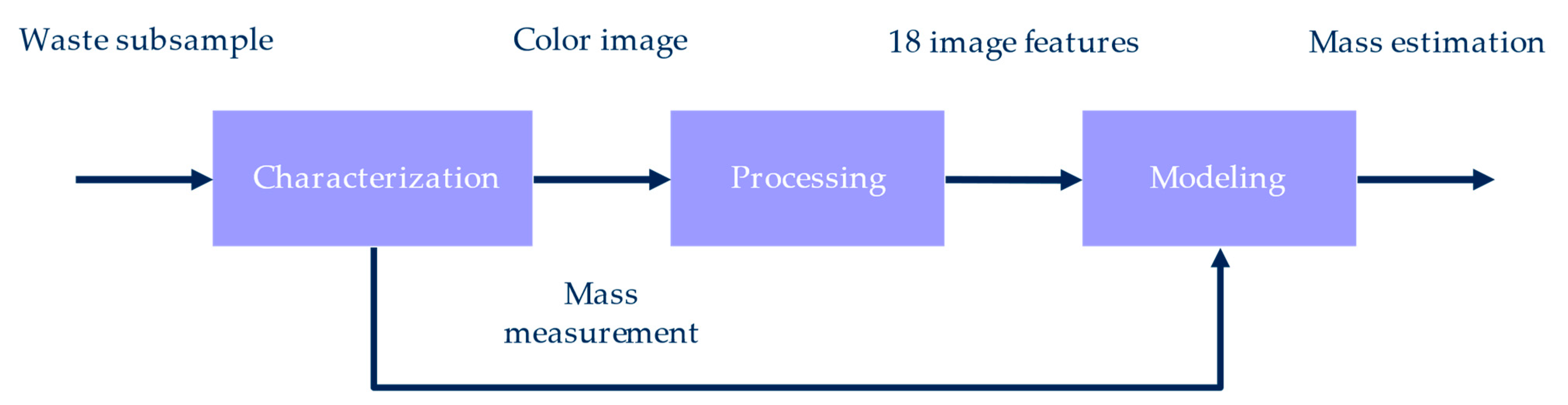
The method to estimate waste mass based on images is shown in Figure 3. Each subsample was characterized by measuring the mass of all the waste particles and acquiring a color image of them. Next, the picture was processed to compute eighteen quantitative features. Mass measurements were used to adjust the visual models.

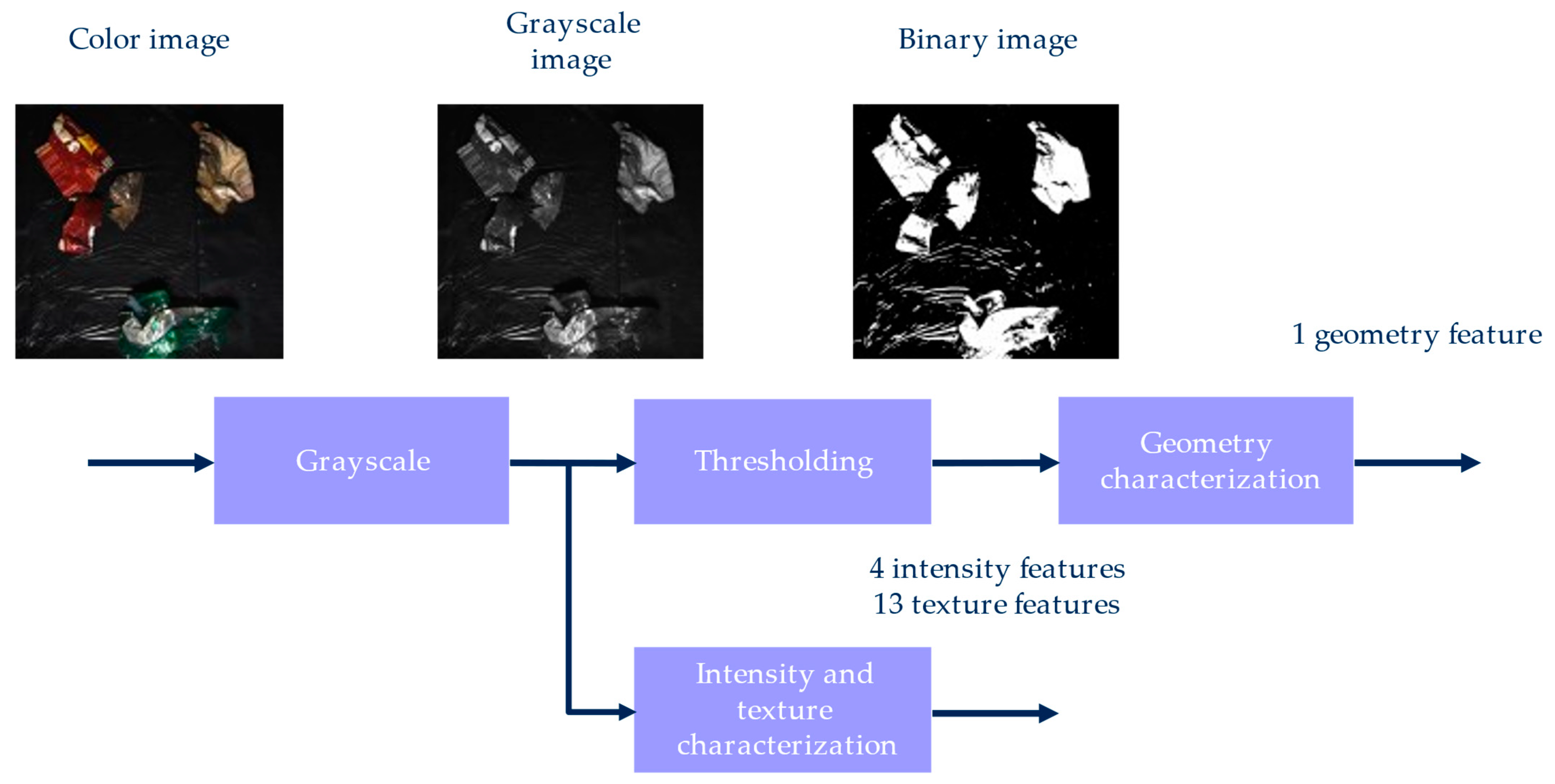
The method for the processing of waste images is summarized in Figure 4. Color images were converted to grayscale, and the image area covered by waste was quantified by counting waste pixels, segmented via thresholding. Furthermore, four intensity and thirteen texture features were computed from the grayscale images.

As previously commented, color and near-infrared cameras are relevant alternatives for material classification. While color cameras capture three monochrome images that form a color image, near-infrared cameras acquire only one. To reduce the dependence of the method on the use of color images, pictures were converted to grayscale. This way, a single monochrome image was obtained per trigger, as for near-infrared cameras. Color images were converted to grayscale by applying the method defined by OpenCV [26]. Grayscale pictures were defined as the linear combination of the red, green, and blue color channels, multiplied by 0.299, 0.587, and 0.114, respectively.

In the collected images, waste particles were generally brighter than the black surface where they were distributed, suggesting the alternative of mass estimation based on images. Waste pixels were segmented via thresholding, a common technique applied to different sectors [1,27,28]. In this study, pixels with a value equal to or higher than a predefined value were classified as waste, and the rest were considered background. Different thresholds were tested to reduce the error of waste segmentation. As result, an intensity level of 40 was chosen (16% of the maximum pixel value). Thresholding provided binary images whose pixel values were 0 (background) or 1 (waste). Next, the number of waste pixels was computed to characterize the image area covered by waste. This geometrical feature has been previously used for material characterization [1,3,4,5] and other applications [28,29].

Intensity and texture features were extracted from the whole image (waste and non-waste pixels). Based on the different intensity between the waste fragments and background, variations in the cover ratio could affect the intensity properties of the whole image, such as its mean value. A higher number of waste particles in the image may also raise the number of adjacent pixels with a significant difference in intensity, corresponding to the edges of waste fragments. Moreover, waste particles could have a different texture than the background, modifying the image texture according to the load proportion. These effects were studied by computing intensity and texture features from all the image pixels.

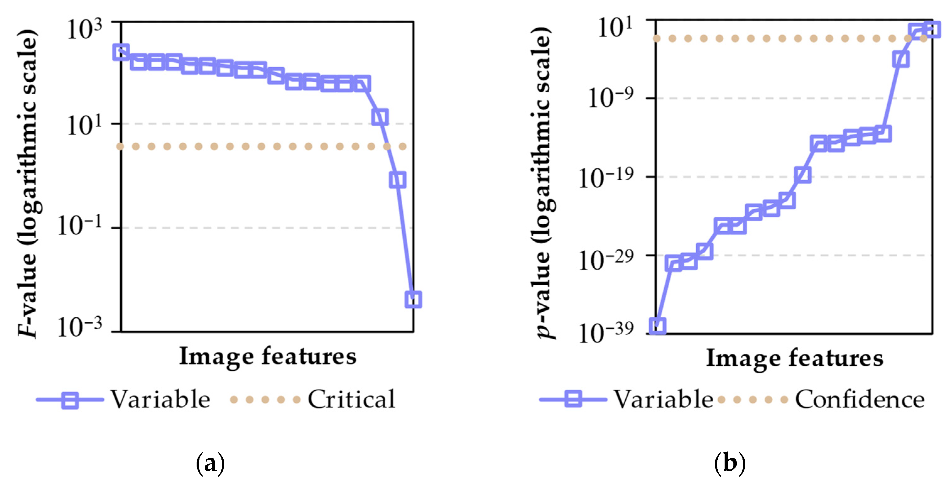
As for the image feature of the number (area) of segmented pixels, intensity and texture properties have been used to characterize materials [30]. In this work, the set of intensity features included the mean, standard deviation, skewness, and kurtosis [31]. These properties are listed in

Table 3. Intensity features extracted from the grayscale waste images [31].

Magnitude	Expression
Mean, μ	${\displaystyle \frac{1}{P}}{\sum }_{p=1}^{P}x\left(p\right)$
Standard deviation, σ	$\sqrt{{\displaystyle \frac{1}{P}}{\sum }_{p=1}^P{\left(x\right(p)-\mu )}^2}$
Skewness	${\displaystyle \frac{\frac{1}{P}{\sum }_{p=1}^P{\left(x\right(p)-\mu )}^3}{{\sigma }^3}}$
Kurtosis	${\displaystyle \frac{\frac{1}{P}{\sum }_{p=1}^P{\left(x\right(p)-\mu )}^4}{{\sigma }^4}}$

, considering a monochrome image of P pixels, where x(p) was the value of pixel p.

Texture characteristics (

Table 4. Texture features extracted from the GLCM of the grayscale waste images [32].

Magnitude	Expression
Angular second moment, energy	${\sum }_{i=1}^N{\sum }_{j=1}^N{p(i,j)}^2$
Contrast	${\sum }_{i=1}^N{\sum }_{j=1}^N{\left(i-j\right)}^{2}p(i,j)$
Correlation	${\sum }_{i=1}^N{\sum }_{j=1}^N{\displaystyle \frac{\left(ij\right)p\left(i,j\right)-{\mu }_x{\mu }_y}{{\sigma }_x{\sigma }_y}}$
Sum of squares, variance	${\sum }_{i=1}^N{\sum }_{j=1}^N{\left(i-{\mu }_x\right)}^2{p}_{ij}$
Inverse difference moment	${\sum }_{i=1}^N{\sum }_{j=1}^N{\displaystyle \frac{p_{ij}}{1+\left|i-j\right|}}$
Sum average	${\sum }_{k=2}^{2N}k{p}_{x+y}\left(k\right)$
Sum variance	${\sum }_{k=2}^{2N}{\left(k-{\mu }_{x+y}\right)}^2{p}_{x+y}\left(k\right)$
Sum entropy	$-{\sum }_{k=2}^{2N}{p}_{x+y}\left(k\right)\mathit{log}{p}_{x+y}\left(k\right)$
Entropy	$-{\sum }_{i=1}^N{\sum }_{j=1}^{N}p(i,j)\mathit{log}p(i,j)$
Difference variance	${\sum }_{k=0}^{N-1}{\left(k-{\mu }_{x-y}\right)}^2{p}_{x-y}\left(k\right)$
Difference entropy	$-{\sum }_{k=0}^{N-1}{p}_{x-y}\left(k\right)\mathit{log}{p}_{x-y}\left(k\right)$
Information measure of correlation I	${\displaystyle \frac{HXY-HXY1}{max(HX,HY)}}$
Information measure of correlation II	$\sqrt{1-\mathit{exp}\left[-2(HXY2-HXY)\right]}$

) comprised the thirteen variables defined by Haralick et al. from the gray-level co-occurrence matrix (GLCM) [32,33]. The GLCM has as many rows and columns as quantized gray values in the image (N). The element in row i and column j, p(i,j), counts the number of times that a pixel of value i is next to a pixel of value j, divided by the total number of instances. GLCMs are computed for a distance d and angle a, which can be 0, 45, 90, and 135° in the case of 2D images. This work used a distance of one pixel and averaged the values for the four pixel angles.

The texture features included three correlation properties to quantify the linear dependence between gray levels of local pixels and their neighbors [32]. The third texture variable (correlation) was complemented with the information measures of correlation I and II for general cases without normal distribution [32,34].

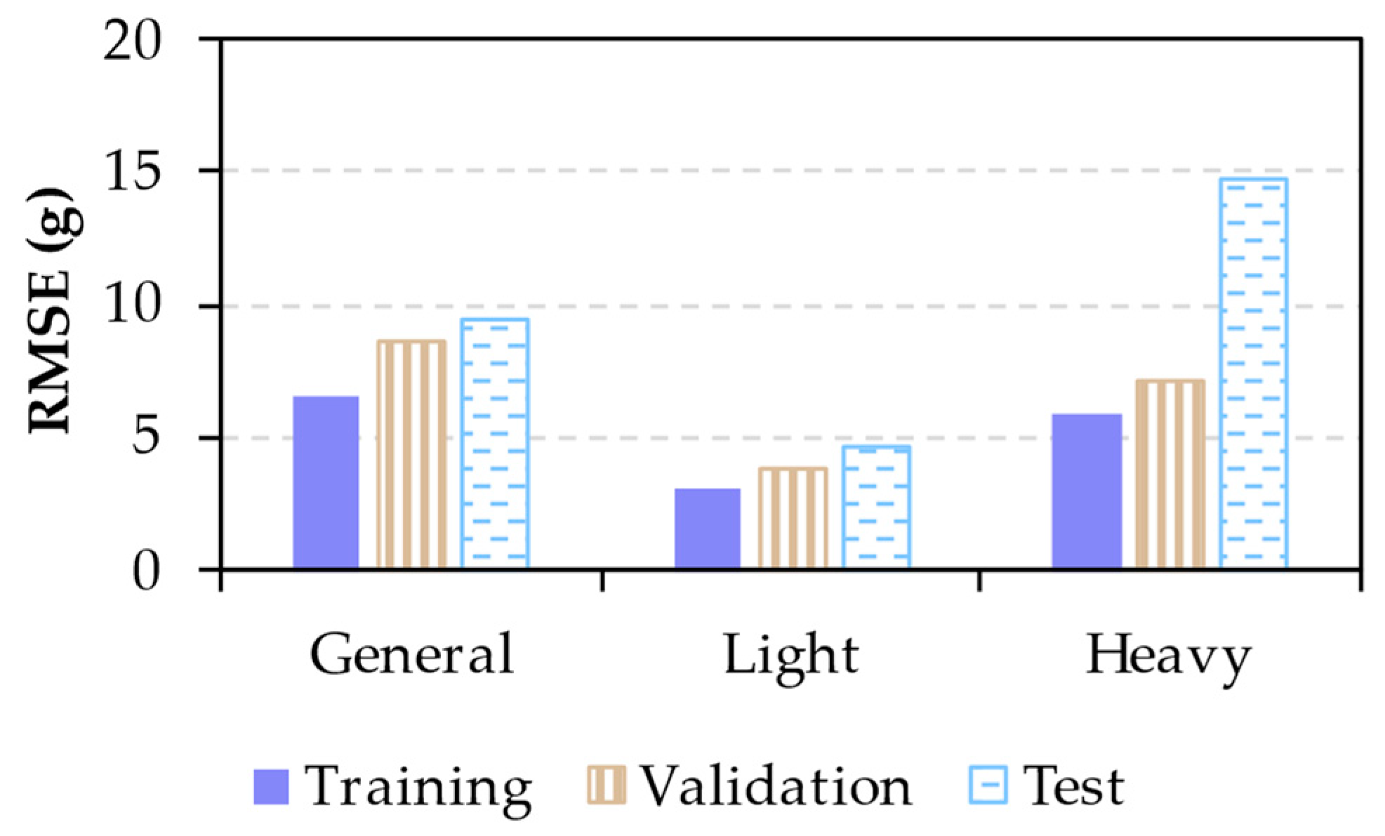
After the steps of characterization and processing, a dataset of 210 subsamples was obtained. Each subsample included a mass measurement and eighteen image features. A previous analysis of the weight values detected asymmetry in the data distribution, with 70% of subsamples weighing less than 22 g (25% of the mass range). This behavior increased the uncertainty about the performance of a general model for all the subsamples. Therefore, three different mass intervals were modeled: general, light, and heavy. Each one of these ranges was split into training and test sets, with 70% and 30% of the subsamples, respectively.

Table 5. Definition of datasets for the modeling of mass.

Dataset	Mass Interval (g)	Subsamples	Training	Test
General	[2.37, 82.40]	210	147	63
Light	[2.37, 22.00)	147	102	45
Heavy	[22.0, 82.40]	63	44	19

lists the characteristics of the datasets.

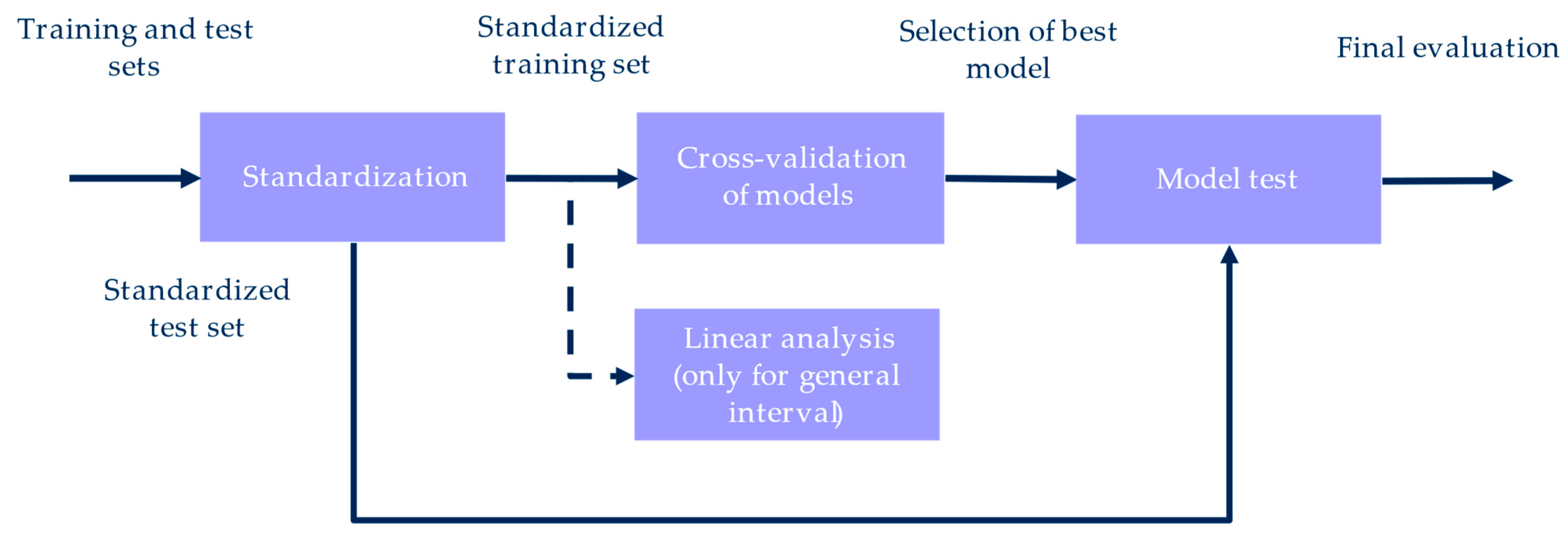
The datasets provided three pairs of training and test sets to model each mass interval. A similar method of machine learning was followed for the three ranges of mass, summarized in Figure 5. The training and test sets were standardized according to the means and standard deviations of the training set. The linear relationship between mass measurements and image features was analyzed with F-tests for the general interval of mass. A cross-validation was applied to the training set to select the best model between different alternatives. Then, the test set was employed as unseen data to perform the final evaluation of the best models.

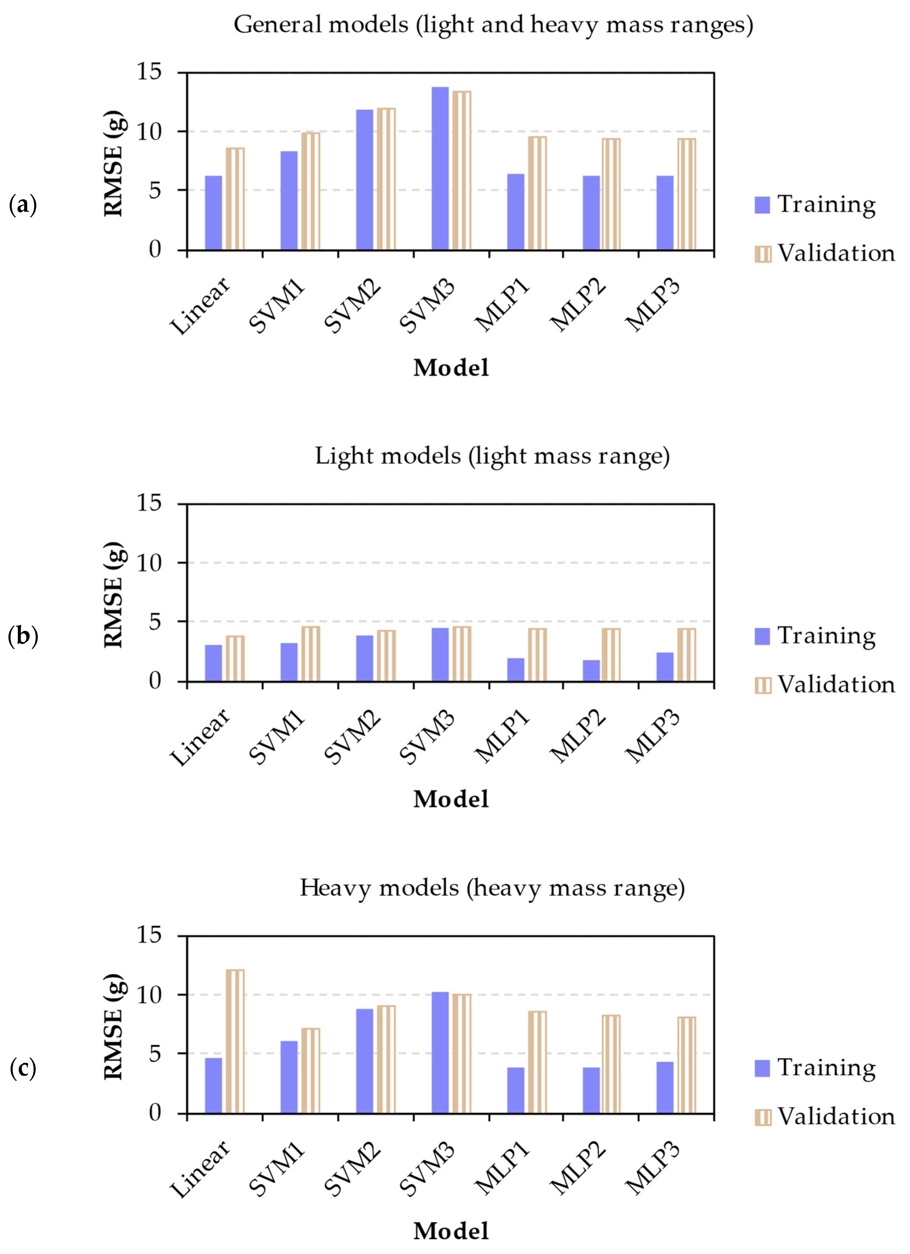
For the three datasets, different options of algorithms and regularization terms were evaluated in the step of cross-validation (

Table 6. Models evaluated during the step of cross-validation.

Model	Algorithm	Regularization Term	Notes
Linear	Linear	-	Ordinary least squares
SVM1	SVM	0.1	Kernel of radial basis function
SVM2		1
SVM3		10
MLP1	MLP	0.1	One hidden layer of 100 neurons
MLP2		1
MLP3		10

). Three algorithms were studied from artificial neural networks: linear, support vector machine (SVM), and multilayer perceptron (MLP). The linear algorithm employed the method of ordinary least squares, SVM used a radial basis function as the kernel, and the MLP was defined with a single hidden layer of one hundred neurons. Three values of the regularization term were studied for SVM and MLP: 0.1, 1, and 10.

A five-fold cross-validation was employed to evaluate the seven models. The training set was divided into five groups, combined to provide five pairs of training and validation subsets. Each training subset was formed by four folds, while its corresponding validation subset included the remaining fold. Models were trained with the training subsets, and the root mean square error (RMSE) of their predictions was computed for the training and validation subsets. The results were averaged for the five different groups and for each algorithm.

As a final evaluation for each mass interval, the model with the lowest RMSE was trained with the whole training set. Next, the RMSE was computed for the training and test sets, and the predicted and actual values were plotted. The performance of the general model was analyzed in more detail, computing its RMSE for the light and heavy subsamples. Apart from the RMSE, the normalized mean absolute error (nMAE) was obtained to compare the results with a previous study [5]. This work was selected due to its study of a similar waste sample, formed by lightweight packaging particles of up to 70 g. The nMAE was computed by dividing the mean absolute error by the average mass of the considered range (Table 5). Finally, the predicted and actual masses of the three models were plotted for their corresponding training and test sets.

The Python programming language (version 3.9) to develop the code for image processing and modeling. With that purpose, the following libraries were employed: OpenCV v4.9.0.80, Scikit-learn v1.4.2, NumPy v1.26.4, SciPy v1.13.0, Mahotas v1.4.13, and Pandas v2.2.2. The computer used was equipped with an Intel Core i7-1165G7 processor (Santa Clara, CA, USA) and a RAM of 16 GB. This processor is a member of the eleventh generation, and it has four cores and frequency of 2.80 GHz.

3. Results and Discussion

3.1. Analysis of Waste Images and Mass Measurements

One color image was acquired per waste subsample, providing a dataset of 210 images with different cover levels. As an example, Figure 6 shows the images of the ten subsamples obtained from the same group of waste particles. The waste bits had variable size and weight, which limited their equal distribution between subsamples for the same cover level and particle group. Most waste fragments were easily distinguished from the background surface by the human eye, although 6% of the subsamples included black fragments that may not be perceived (Figure 7a). The histograms of the grayscale images from Figure 6 are included in Figure 7b, averaged for each cover level. The effect of background bits was observed between the pixel values of 0 and 50. Their frequency increased with the reduction in the cover level due to the higher proportion between the background and waste pixels.

Figure 8 includes the mass of each subsample and the three quartiles of the general dataset, illustrating the asymmetric distribution. The consecutive characterizations of the same group of waste particles, in decreasing order of load level, generated a pattern that repeats every ten values. This signature is shown in more detail for the subsamples from 1 to 10 (Figure 9a) and from 51 to 60 (Figure 9b). Figure 9 also includes the theoretical values for a uniform distribution of mass between cover levels.

The mass differences between waste fragments limited their distribution along the subsamples, modifying the experimental values with respect to the theoretical and uniform assumption (Figure 9). The subsamples obtained for the same group of particles and different cover levels may have similar weights, such as subsamples 3 (medium-high) and 5 (low-medium). This effect was also measured between different groups of waste fragments, for example subsamples 1 (high) and 52 (medium-high). To study in more detail the intersection between cover levels, Figure 10 shows their boxplots with quartiles, minimum, and maximum values.

All the cover levels had mass values in common, but their quartile ranges were exclusive except for the low-medium and low classes. The intersection between cover levels increased for lower classes due to the distribution procedure of waste particles employed in this work (Table 2). While the cover area was reduced by 50% between the high and medium-high classes, it only decreased by 34% between the medium-high and low-medium levels and by 24% for the low-medium and low scenarios.

The overlapping between load classes limited their viability as descriptors of image mass. However, their sampling method enabled the generation of a diverse image dataset, with variations in the number of waste particles. The rest of the study focused on the analysis of mass instead of cover classes, which provided a more accurate variable to study.

3.2. Analysis of Linear Relationships Between Mass Measurements and Image Features

The linear relationship between mass measurements and image features was evaluated for the general training set using one F-test per variable. A confidence level of 0.05 was defined, obtaining a critical F-value of 3.91. Figure 11 includes the F-values and p-values computed for each image feature. Of the total, 89% of the properties had a linear relationship with mass, including visual variables from the three considered types, i.e., geometry, intensity, and texture. Only two texture properties did not share this relationship: the energy and the information measure of correlation I.

For each feature type, the characteristics with a stronger linear dependency on mass were the geometry area (Figure 12a), intensity mean (Figure 12b), and texture sum entropy (Figure 12c). The evolution of these properties along the four cover levels of a group of waste fragments is shown in Figure 13.

While pixel segmentation was applied to compute the area covered by waste in the image, it was not employed to extract the intensity and texture characteristics. With or without segmentation, image features linearly dependent on mass were obtained. This work proposed the novel application of intensity and texture features for mass monitoring, achieving promising results during the analysis of their linear dependency.

3.3. Cross-Validation of Mass Models Based on Image Features

The models were adjusted to estimate the total mass of waste particles captured in an image. With that purpose, the images were processed to extract eighteen visual properties used as input of the models. Seven different alternatives were cross-validated by employing the standardized training set, split into five pairs of training and validation subsets. This process was repeated for the three mass intervals, whose RMSEs are shown in Figure 14.

While error values for the general mass interval ranged between 6 and 14 g, the light and heavy models had lower errors, from 1 to 5 and 3 to 13 g, respectively. The error reduction was repeated when selecting the best alternative (lowest validation error) for each mass interval. The models with the lowest RMSE employed linear (general and light intervals) and SVM algorithms, using a regularization parameter of 0.1 (heavy interval) in the latter case. These models reached validation RMSEs of 8.63 (general), 3.84 (light), and 7.11 (heavy) g. The results could support the hypothesis of using specific models for the light and heavy mass intervals to improve the estimation performance. However, the general model could have a different RMSE for the light and heavy subsamples, requiring additional tests to confirm the theory. This aspect is analyzed later with the final evaluation of the best mass models.

This work conducted an experimental campaign where 146 training samples were characterized, matching the order of previous sorting studies with 122 [25] and 400 [15] data points. Due to the asymmetric distribution of the mass samples, model performance was analyzed for the light and heavy ranges, aiming to provide a higher level of detail. The error of the specific models was lower for the light range, which could be due to its higher number of training samples (102) with respect to the heavy range (44). The lower number of data points for the heavy range was promoted by the study of different cover levels. The sampling of each group of waste particles was characterized by the collection of seven measurements of low and low-medium cover levels and three medium-high and high data points. According to Figure 10, the reduction in load class decreased the mass average, and thus, a higher proportion of light samples could be collected. Moreover, this study focused on the monitoring of mass for low-density materials, using post-consumer plastic film with 84–94% of LDPE in weight. Heavier samples could be also collected by considering waste samples with higher densities.

By comparing training and validation errors, overfitting was detected for the linear and MLP algorithms. The overfitting of SVM models was removed with higher regularization parameters, although they barely affected the results of the MLP algorithm. To study in more detail the performance of the models, the validation RMSE was averaged for each algorithm, and the variation was computed with respect to the best algorithm of each mass interval (

Table 7. Average validation RMSE for the model algorithms and variation with respect to the best algorithm of each mass interval.

Mass Interval	Algorithm	Average Validation RMSE (g)	Variation of Validation RMSE (%)
General	Linear	8.63	-
	SVM	11.74	36
	MLP	9.45	10
Light	Linear	3.84	-
	SVM	4.53	18
	MLP	4.43	15
Heavy	Linear	12.06	45
	SVM	8.76	5
	MLP	8.32	-

). The error difference between algorithms was 25 ± 20%, matching the order of previous models of mass (18 ± 11%, [5]). From the literature review, the best machine learning models for other applications of material flow characterization achieved accuracies with a maximum difference of 51% [14]. Additionally, the accuracy of machine vision techniques for food sorting and grading varied up to 37% [35].

3.4. Final Evaluation of the Best Models of Mass

The model with the lowest validation error for each mass interval was evaluated employing unseen data (test set). With that purpose, the model was trained with the whole training set, and its RMSE was computed for the training and test sets. Figure 15 shows the results for the three mass ranges, together with the validation RMSE previously obtained. The error exhibited usual behavior for the general and light ranges, with a slight increase from the training set to the validation and test groups. Nevertheless, the RMSE was doubled between the validation and test sets of the heavy range. Similar trends were promoted by groups with a reduced volume, as in the case of the heavy set (41 samples for training and 21 for testing), 58% and 70% smaller than the light and general groups, respectively. Due to the low number of samples, the data may have different behavior in the training and test sets, which could reduce the performance of the test.

To compare the performance of the three models in the same mass intervals, the test RMSE of the general model was computed for the light and heavy subsamples (

Table 8. RMSE for the general, light, and heavy models considering the light and heavy test subsamples.

Mass Interval	Model Type	Model	Test RMSE (g)	Test nMAE
Light	General	Linear	6.18	0.43
	Light	Linear	4.67	0.28
Heavy	General	Linear	13.78	0.93
	Heavy	SVM1	14.72	1.11

). The nMAE was also obtained to compare the performance of the models with the results from a previous work.

The specific model adjusted for the light interval of mass reduced the error by 24% with respect to the general model, achieving an RMSE of 4.67 g. The general model differed with the addition of heavy samples in its datasets. Therefore, visual properties could depend on the mass interval, and the adjustment of a specific model for the light range improved the estimation performance.

However, the heavy model did not enhance the RMSE of the general model for the heavy subsamples, which was increased by 7%. In this case, the reduced number of data points promoted the error rise for the specific model. Although light and heavy subsamples could have different image characteristics, the higher volume of light subsamples provided a lower RMSE for the general model.

Another study achieved an nMAE of 0.24 [5] using shape characteristics extracted from 2D and 3D images. By contrast, this work reached a similar performance for the light mass interval (nMAE of 0.28) using a novel method with three main differences: (1) mass was predicted for images with one or more particles, (2) 3D variables were not used, and (3) only one of the 2D shape features from the other work (area) was employed, while integrating new intensity and texture variables for the whole image. Furthermore, both studies reported an error increase for heavier particle ranges.

To conclude, Figure 16 includes the predicted and actual values of mass during the training and testing of the general and specific models. The error reduction of the light model with respect to the general one is shown as a higher concentration of data points towards the line of perfect estimation. This behavior was shared by the heavy model for the subsamples between 22 and 40 g, although deviation was increased for mass values higher than 55 g. These data points had higher errors for the heavy model than for the general one, resulting in an overall increase of the RMSE.

4. Conclusions

This work analyzed the modeling of mass using 2D images for its application during sorting processes. A sample of post-consumer plastic film was collected from a material recovery facility, and different cover ratios were studied by modifying the number of waste particles in each image. Waste pixels were identified and quantified, and intensity and texture features were extracted from the whole image (waste and non-waste pixels). The models were adjusted to predict the total mass of the particles captured in a picture, and the relationship between mass and image features was evaluated using linear F-tests. Due to the asymmetric distribution of the weight measurements, three mass intervals were studied: general, light, and heavy. For each one, three regression algorithms were analyzed: linear, SVM, and MLP. The performance of the models was evaluated using a training–test split and a cross-validation.

The main conclusions of the study are presented next. Mass varied according to cover levels, although they overlapped in part of the weight range. Intensity and texture features had a linear relationship with mass, similar to the conventional characteristic of particle size but without requiring the segmentation of waste pixels in the image. The weight models were adjusted based on the image characteristics, providing an average error of 9 g for particles between 2 and 82 g. This novel method matched results from a previous work, which also used additional information (3D measurements).

Future studies may focus on the extraction of intensity and texture features from waste particles, instead of the whole image. This could provide a detailed characterization of the material to increase the accuracy of mass estimation. For example, the application of these features could be analyzed for the detection of wrinkled packages in sorting processes, which may have a higher apparent density than flat elements. In this study, model accuracy decreased for heavier particles, which could be studied in more detail by increasing the number of data points with additional tests. Finally, models could be generalized or fine-tuned for different material streams.