
A New Productivity Evaluation Method for Horizontal Wells in Offshore Low-Permeability Reservoir Based on Modified Theoretical Model

 ,
,
Abstract
1. Introduction
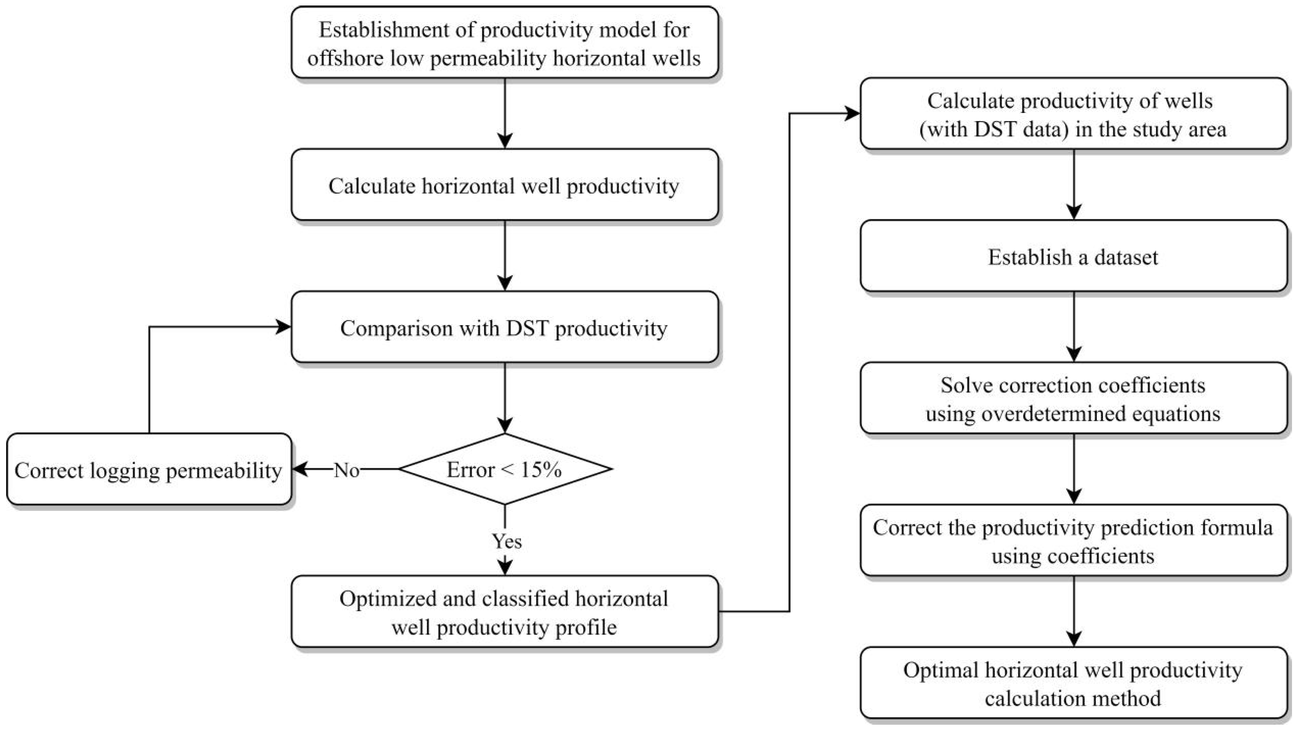
2. Workflow
3. Establishment of a Horizontal Well Productivity Function for Offshore Low-Permeability Reservoirs
4. Horizontal Well Productivity Classification and Determination of Interference Factors
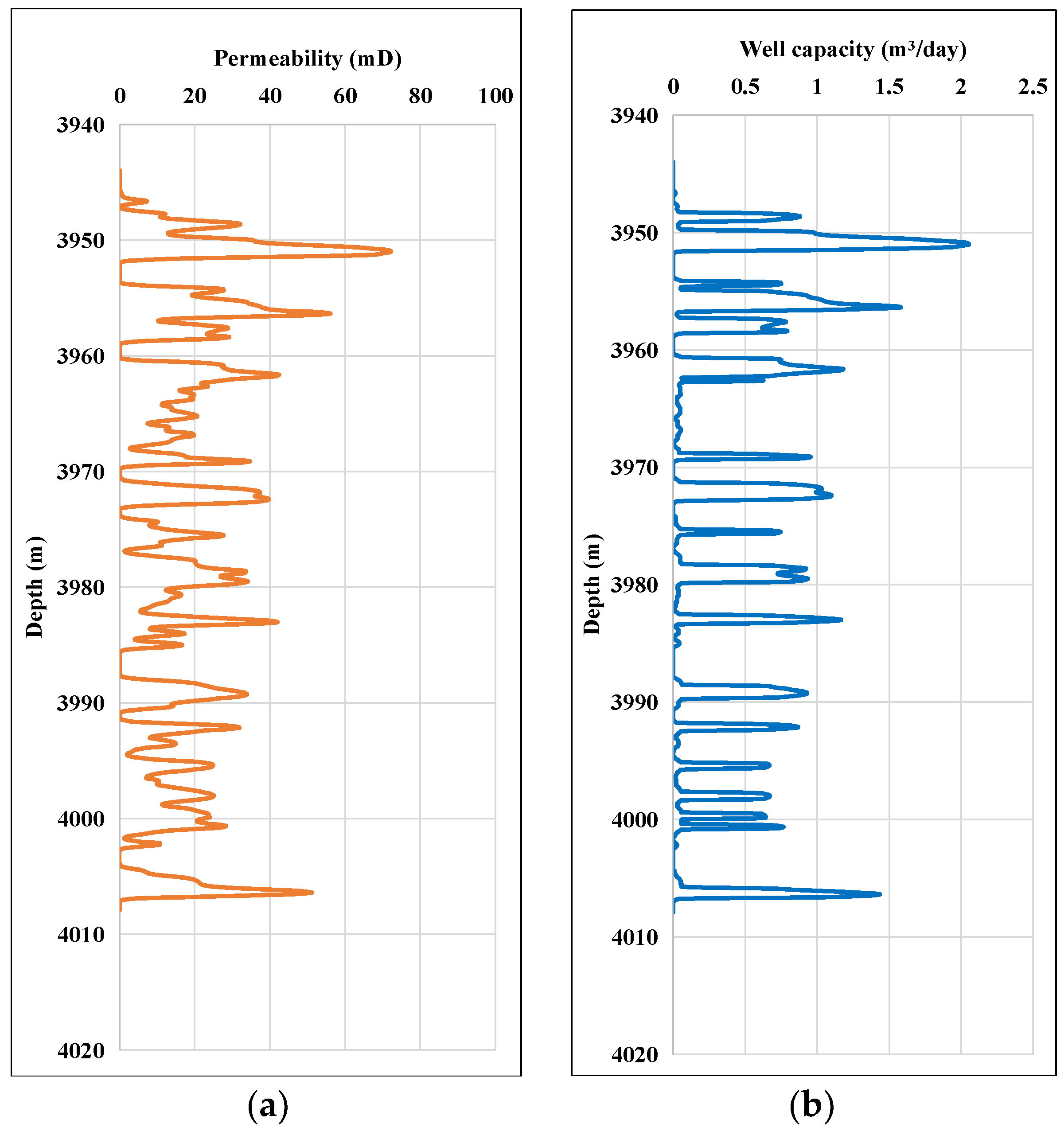
4.1. Establishment and Classification of Productivity Profiles for Horizontal Wells
4.2. Productivity Prediction Optimization Based on Overdetermined System
5. Case Study
5.1. Reservoir Background
5.2. Determining Correction Coefficients by Overdetermined Equations
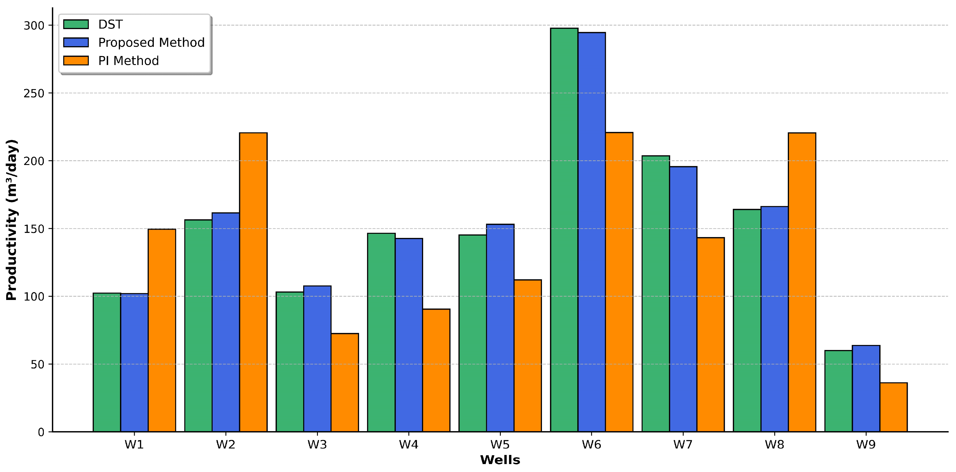
5.3. Prediction Accuracy Comparison
6. Conclusions and Recommendations
- By incorporating key factors such as the threshold pressure gradient, stress sensitivity, skin factor, and formation heterogeneity into a nonlinear seepage mathematical model, this study derived a robust formula for evaluating horizontal well productivity. This formula enables a detailed depiction of productivity profiles at the resolution level of logging curves, providing a more accurate representation of reservoir behavior.
- Based on the differences in permeability distribution of horizontal wells, the productivity of individual wells was classified. The introduction of overdetermined equation concepts allowed the derivation of correction coefficients suitable for the productivity evaluation equation of these horizontal wells: x1 = 3.3182, x2 = 0.7720, x3 = 1.0327. This approach resolved the issue of significant discrepancies between the horizontal well productivity formula and DST productivity data.
- A case study on offshore low-permeability reservoirs in the eastern South China Sea region, through evaluating the productivity of nine horizontal wells in the study area, demonstrated that the method of this study significantly improved the accuracy of productivity evaluation. Compared to the traditional PI method, the accuracy increased from 65.80% to 96.82%.
Author Contributions
Funding
Data Availability Statement
Acknowledgments
Conflicts of Interest
References
- Behrenbruch, P. Offshore Oilfield Development Planning. J. Pet. Technol. 1993, 45, 735–743. [Google Scholar] [CrossRef]
- Black, A.; Saunders, G. Offshore Gas Field Development—The Ripple Effect. APPEA J. 2018, 58, 695. [Google Scholar] [CrossRef]
- Darche, G.; Marmier, R.; Samier, P.; Bursaux, R.; Guillonneau, N.; Long, J.; Kalunga, H.; Zaydullin, R.; Cao, H. Integrated Asset Modeling of a Deep-Offshore Subsea Development Using 2 Complementary Reservoir-Surface Coupling Workflows. In Proceedings of the SPE Reservoir Simulation Conference, Galveston, TX, USA, 10 April 2019; p. D011S005R004. [Google Scholar]
- Zou, C.; Zhai, G.; Zhang, G.; Wang, H.; Zhang, G.; Li, J.; Wang, Z.; Wen, Z.; Ma, F.; Liang, Y.; et al. Formation, Distribution, Potential and Prediction of Global Conventional and Unconventional Hydrocarbon Resources. Pet. Explor. Dev. 2015, 42, 14–28. [Google Scholar] [CrossRef]
- Tavallali, M.S.; Karimi, I.A. Integrated Oil-Field Management: From Well Placement and Planning to Production Scheduling. Ind. Eng. Chem. Res. 2016, 55, 978–994. [Google Scholar] [CrossRef]
- Devine, M.D.; Lesso, W.G. Models for the Minimum Cost Development of Offshore Oil Fields. Manag. Sci. 1972, 18, B-378–B-387. [Google Scholar] [CrossRef]
- Rogner, H.-H. An Assessment of World Hydrocarbon Resources. Annu. Rev. Energy Environ. 1997, 22, 217–262. [Google Scholar] [CrossRef]
- Morooka, C.K.; Galeano, Y.D. Systematic Design For Offshore Oilfield Development; OnePetro: Richardson, TX, USA, 1999. [Google Scholar]
- Lu, W.; Yang, Y.; Liu, J.; Jia, Z.; Wang, H. Comparison of Different Offshore Oil Field Development Concepts; OnePetro: Richardson, TX, USA, 2006. [Google Scholar]
- Gupta, V.; Grossmann, I.E. Development Planning of Offshore Oilfield Infrastructure. In Alternative Energy Sources and Technologies: Process Design and Operation; Martín, M., Ed.; Springer International Publishing: Cham, Switzerland, 2016; pp. 33–87. ISBN 978-3-319-28752-2. [Google Scholar]
- Gupta, V.; Grossmann, I.E. Offshore Oilfield Development Planning under Uncertainty and Fiscal Considerations. Optim. Eng. 2017, 18, 3–33. [Google Scholar] [CrossRef]
- Karimov, V.M.; Sharifov, J.J.; Zeynalova, S.A. Intensification of Oil Production in Long-Term Developed Offshore Fields. J. Geol. Geogr. Geoecol. 2023, 32, 276–282. [Google Scholar] [CrossRef]
- Krueger, R.F. An Overview of Formation Damage and Well Productivity in Oilfield Operations. J. Pet. Technol. 1986, 38, 131–152. [Google Scholar] [CrossRef]
- Joshi, S.D. Augmentation of Well Productivity With Slant and Horizontal Wells (Includes Associated Papers 24547 and 25308). J. Pet. Technol. 1988, 40, 729–739. [Google Scholar] [CrossRef]
- Veeken, C.A.M.; Davies, D.R.; Kenter, C.J.; Kooijman, A.P. Sand Production Prediction Review: Developing an Integrated Approach. In Proceedings of the SPE Annual Technical Conference and Exhibition, Dallas, TX, USA, 6–9 October 1991; p. SPE-22792-MS. [Google Scholar]
- Guo, B.; Sun, K.; Ghalambor, A. Well Productivity Handbook; Elsevier: Amsterdam, The Netherlands, 2014; ISBN 978-0-12-799992-0. [Google Scholar]
- Wu, Z.; Sun, Z.; Shu, K.; Jiang, S.; Gou, Q.; Chen, Z. Mechanism of Shale Oil Displacement by CO2 in Nanopores: A Molecular Dynamics Simulation Study. Adv. Geo-Energy Res. 2024, 11, 141–151. [Google Scholar] [CrossRef]
- Al-Rbeawi, S.; Artun, E. Fishbone Type Horizontal Wellbore Completion: A Study for Pressure Behavior, Flow Regimes, and Productivity Index. J. Pet. Sci. Eng. 2019, 176, 172–202. [Google Scholar] [CrossRef]
- Dong, Y.; Ju, B.; Yang, Y.; Wang, J.; Ma, S.; Brantson, E.T. A Semi-Analytical Method for Optimizing the Gas and Water Bidirectional Displacement in the Tilted Fault Block Reservoir. J. Pet. Sci. Eng. 2021, 198, 108213. [Google Scholar] [CrossRef]
- Al-Kabbawi, F.A.A. Simple Pseudo-Steady State Productivity Index Correlations for Infinite-Conductivity Horizontal Wells Based on a Rigorous, Semi-Analytical Model. Geoenergy Sci. Eng. 2024, 233, 212534. [Google Scholar] [CrossRef]
- Jreou, G.N.S. Productivity Index of Horizontal Well in Mishrif Formation of Buzurgan Oil Field—Case Study. Int. Rev. Appl. Sci. Eng. 2021, 12, 301–311. [Google Scholar] [CrossRef]
- Xiong, S.; Liu, S.; Weng, D.; Shen, R.; Yu, J.; Yan, X.; He, Y.; Chu, S. A Fractional Step Method to Solve Productivity Model of Horizontal Wells Based on Heterogeneous Structure of Fracture Network. Energies 2022, 15, 3907. [Google Scholar] [CrossRef]
- Jia, X.; Sun, Z.; Lei, G.; Yao, C. Model for Predicting Horizontal Well Transient Productivity in the Bottom-Water Reservoir with Finite Water Bodies. Energies 2023, 16, 1952. [Google Scholar] [CrossRef]
- Ke, W.; Luo, W.; Miao, S.; Chen, W.; Hou, Y. A Transient Productivity Prediction Model for Horizontal Wells Coupled with Oil and Gas Two-Phase Seepage and Wellbore Flow. Processes 2023, 11, 2012. [Google Scholar] [CrossRef]
- Bi, G.; Cui, Y.; Wu, J.; Ren, Z.; Han, F.; Wang, X.; Li, M. Unsteady Productivity Prediction for Three-Dimensional Horizontal Well in Anisotropic Reservoir. Geofluids 2022, 2022, 2697311. [Google Scholar] [CrossRef]
- Wu, Z.; Jiang, S.; Xie, C.; Chen, K.; Zhang, Z. Production Performance of Multiple-Fractured Horizontal Well Based on Potential Theory. J. Energy Resour. Technol. 2022, 144, 103005. [Google Scholar] [CrossRef]
- Cao, L.; Li, X.; Zhang, J.; Luo, C.; Tan, X. Dual-Porosity Model of Rate Transient Analysis for Horizontal Well in Tight Gas Reservoirs with Consideration of Threshold Pressure Gradient. J. Hydrodyn. 2018, 30, 872–881. [Google Scholar] [CrossRef]
- Hao, F.; Cheng, L.S.; Hassan, O.; Hou, J.; Liu, C.Z.; Feng, J.D. Threshold Pressure Gradient in Ultra-Low Permeability Reservoirs. Pet. Sci. Technol. 2008, 26, 1024–1035. [Google Scholar] [CrossRef]
- Prada, A.; Civan, F. Modification of Darcy’s Law for the Threshold Pressure Gradient. J. Pet. Sci. Eng. 1999, 22, 237–240. [Google Scholar] [CrossRef]
- Yao, J.; Ding, Y.; Sun, H.; Fan, D.; Wang, M.; Jia, C. Productivity Analysis of Fractured Horizontal Wells in Tight Gas Reservoirs Using a Gas-Water Two-Phase Flow Model with Consideration of a Threshold Pressure Gradient. Energy Fuels 2023, 37, 8190–8198. [Google Scholar] [CrossRef]
- Dong, M.; Shi, X.; Bai, J.; Yang, Z.; Qi, Z. A Novel Model for Well Production Performance Estimate in Low-Permeability and Tight Reservoirs Considering Stress Sensitivity. J. Energy Resour. Technol. 2020, 142, 093002. [Google Scholar] [CrossRef]
- Guo, J.; Wang, H.; Zhang, L.; Li, C. Pressure Transient Analysis and Flux Distribution for Multistage Fractured Horizontal Wells in Triple-Porosity Reservoir Media with Consideration of Stress-Sensitivity Effect. J. Chem. 2015, 2015, 212901. [Google Scholar] [CrossRef]
- Dong, M.; Yue, X.; Shi, X.; Ling, S.; Zhang, B.; Li, X. Effect of Dynamic Pseudo Threshold Pressure Gradient on Well Production Performance in Low-Permeability and Tight Oil Reservoirs. J. Pet. Sci. Eng. 2019, 173, 69–76. [Google Scholar] [CrossRef]
- Islamov, R.; Bondarenko, A.V.; Korobov, G.Y.; Podoprigora, D.G. Complex algorithm for developing effective kill fluids for oil and gas condensate reservoirs. Int. J. Civ. Eng. Technol. 2019, 10, 2697–2713. [Google Scholar]
- Zhang, Y.; Liu, X.; Li, D.; Chang, L.; Liu, G.; Dou, Z.; Hou, H.; Zhao, X. Physical Simulation Experiment Method of Water Breakthrough Mechanism and Plugging Effect of Horizontal Well in Tight Reservoir. Energy Rep. 2022, 8, 9610–9617. [Google Scholar] [CrossRef]
- Islamov, S.; Islamov, R.; Shelukhov, G.; Sharifov, A.; Sultanbekov, R.; Ismakov, R.; Agliullin, A.; Ganiev, R. Fluid-Loss Control Technology: From Laboratory to Well Field. Processes 2024, 12, 114. [Google Scholar] [CrossRef]
- Belousov, A.; Lushpeev, V.; Sokolov, A.; Sultanbekov, R.; Tyan, Y.; Ovchinnikov, E.; Shvets, A.; Bushuev, V.; Islamov, S. Hartmann–Sprenger Energy Separation Effect for the Quasi-Isothermal Pressure Reduction of Natural Gas: Feasibility Analysis and Numerical Simulation. Energies 2024, 17, 2010. [Google Scholar] [CrossRef]
- Huang, S.; Kang, B.; Cheng, L.; Zhou, W.; Chang, S. Quantitative Characterization of Interlayer Interference and Productivity Prediction of Directional Wells in the Multilayer Commingled Production of Ordinary Offshore Heavy Oil Reservoirs. Pet. Explor. Dev. 2015, 42, 533–540. [Google Scholar] [CrossRef]
- Dasheng, Q.; Bailin, P. Physical Experiment Research of Mechanical Sand Control for Tarim Donghe Oilfield. Pet. Sci. Technol. 2009, 27, 952–958. [Google Scholar] [CrossRef]
- Kadeethum, T.; Salimzadeh, S.; Nick, H.M. An Investigation of Hydromechanical Effect on Well Productivity in Fractured Porous Media Using Full Factorial Experimental Design. J. Pet. Sci. Eng. 2019, 181, 106233. [Google Scholar] [CrossRef]
- Duan, X.; Xu, Y.; Xiong, W.; Hu, Z.; Gao, S.; Chang, J.; Ge, Y. Experimental and Numerical Study on Gas Production Decline Trend under Ultralong-Production-Cycle from Shale Gas Wells. Sci. Rep. 2023, 13, 10726. [Google Scholar] [CrossRef]
- Ertekin, T. Principles of Numerical Simulation of Oil Reservoirs—An Overview. In Heavy Crude Oil Recovery; Okandan, E., Ed.; Springer: Dordrecht, The Netherlands, 1984; pp. 379–407. ISBN 978-94-009-6142-5. [Google Scholar]
- Chen, Z.; Huan, G.; Ma, Y. Computational Methods for Multiphase Flows in Porous Media; Computational Science & Engineering; Society for Industrial and Applied Mathematics: Philadelphia, PA, USA, 2006; ISBN 978-0-89871-606-1. [Google Scholar]
- Chen, Z. Reservoir Simulation: Mathematical Techniques in Oil Recovery; CBMS-NSF Regional Conference Series in Applied Mathematics; SIAM/Society for Industrial and Applied Mathematics: Philadelphia, PA, USA, 2007; ISBN 978-0-89871-640-5. [Google Scholar]
- Hu, J.; Zhang, C.; Rui, Z.; Yu, Y.; Chen, Z. Fractured Horizontal Well Productivity Prediction in Tight Oil Reservoirs. J. Pet. Sci. Eng. 2017, 151, 159–168. [Google Scholar] [CrossRef]
- Sun, F.; Yao, Y.; Li, G.; Li, X. Effect of Physical Heating on Productivity of Cyclic Superheated Steam Stimulation Wells. J. Pet. Explor. Prod. Technol. 2019, 9, 1203–1210. [Google Scholar] [CrossRef]
- Li, Y.; Wang, B.; Wang, J.; Zaki, K.; Wu, R.; Barnum, B.; Rijken, P.; Guyaguler, B. Accurate Production Forecast and Productivity Decline Analysis Using Coupled Full-Field and Near-Wellbore Poromechanics Modeling. In Proceedings of the SPE Reservoir Simulation Conference, Galveston, TX, USA, 29 March 2023; p. D021S008R001. [Google Scholar]
- Roque, W.L.; Araújo, C.P. Production Simulations Based on a Productivity Potential Proxy Function: An Application to UNISIM-I-D and PUNQ-S3 Synthetic Reservoirs. J. Pet. Explor. Prod. Technol. 2021, 11, 399–410. [Google Scholar] [CrossRef]
- Zhang, D.; Zhang, L.; Tang, H.; Zhao, Y. Fully Coupled Fluid-Solid Productivity Numerical Simulation of Multistage Fractured Horizontal Well in Tight Oil Reservoirs. Pet. Explor. Dev. 2022, 49, 382–393. [Google Scholar] [CrossRef]
- Jing, W.; Xiao, L.; Haixia, H.; Wei, L. Productivity Prediction and Simulation Verification of Fishbone Multilateral Wells. Geofluids 2022, 2022, 3415409. [Google Scholar] [CrossRef]
- Maschio, C.; Schiozer, D.J. A New Procedure for Well Productivity and Injectivity Calibration to Improve Short-Term Production Forecast. Geoenergy Sci. Eng. 2023, 229, 212105. [Google Scholar] [CrossRef]


| Calculation Methods | Well No. | Calculated Productivity (m3/d) | Productivity by DST (m3/d) | Error (%) | Average Error (%) |
|---|---|---|---|---|---|
| Horizontal well productivity formula (Joshi formula) | 1 | 258.5 | 210.9 | 22.6 | 44.3 |
| 2 | 180.1 | 123.5 | 45.8 | ||
| 3 | 289.5 | 220.6 | 31.2 | ||
| 4 | 455.7 | 290.2 | 57.0 | ||
| 5 | 151.1 | 74.6 | 102.5 | ||
| 6 | 388.8 | 284.3 | 36.8 | ||
| 7 | 310.1 | 236.9 | 30.9 | ||
| 8 | 254.4 | 176.8 | 43.9 | ||
| 9 | 225.6 | 385.3 | 41.4 | ||
| 10 | 190.8 | 145.6 | 31.0 | ||
| Horizontal well productivity formula (The proposed formula) | 1 | 246.7 | 210.9 | 17.0 | 20.2 |
| 2 | 148.8 | 123.5 | 20.5 | ||
| 3 | 260.1 | 220.6 | 17.9 | ||
| 4 | 350.5 | 290.2 | 20.8 | ||
| 5 | 101.5 | 74.6 | 36.1 | ||
| 6 | 304.3 | 284.3 | 7.0 | ||
| 7 | 287.8 | 236.9 | 21.5 | ||
| 8 | 225.6 | 176.8 | 27.6 | ||
| 9 | 430.2 | 385.3 | 11.7 | ||
| 10 | 178.2 | 145.6 | 22.4 |
| Measured Depth (m) | Permeability (mD) | Porosity (%) | Stress Sensitivity Factor | Threshold Pressure Gradient | Qi (m3/d) | |
|---|---|---|---|---|---|---|
| Average | 3975.94 | 15.23 | 9.90 × 10⁻² | 1.03 × 10⁻³ | 7.33 × 10⁻¹ | 3.95 × 10⁻¹ |
| Max value | 4007.88 | 72.22 | 1.46 × 10⁻¹ | 1.04 × 10⁻³ | 7 | 2.05 × 100 |
| Min value | 3944.00 | 0.01 | 1.83 × 10⁻² | 1.03 × 10⁻³ | 9.69 × 10⁻⁴ | 0 |
| Amount | 512 | |||||
| W1 | W2 | W3 | W4 | W5 | W6 | W7 | W8 | W9 | |
|---|---|---|---|---|---|---|---|---|---|
| Drill Stem Test (m3/d) | 102.3 | 156.3 | 103.1 | 146.5 | 145.2 | 297.8 | 203.6 | 164 | 60 |
| The Proposed Method (m3/d) | 102 | 161.5 | 107.6 | 142.6 | 153.1 | 294.6 | 195.6 | 166.2 | 63.7 |
| PI Method (m3/d) | 149.5 | 220.6 | 72.5 | 90.5 | 112.1 | 220.8 | 143.2 | 220.5 | 36.1 |
| Accuracy of proposed method (%) | 99.71 | 96.67 | 95.64 | 97.34 | 94.56 | 98.93 | 96.07 | 98.66 | 93.83 |
| Accuracy of PI method (%) | 53.86 | 58.86 | 70.32 | 61.77 | 77.20 | 74.14 | 70.33 | 65.55 | 60.17 |
Disclaimer/Publisher’s Note: The statements, opinions and data contained in all publications are solely those of the individual author(s) and contributor(s) and not of MDPI and/or the editor(s). MDPI and/or the editor(s) disclaim responsibility for any injury to people or property resulting from any ideas, methods, instructions or products referred to in the content. |
© 2024 by the authors. Licensee MDPI, Basel, Switzerland. This article is an open access article distributed under the terms and conditions of the Creative Commons Attribution (CC BY) license (https://creativecommons.org/licenses/by/4.0/).
Share and Cite
Li, L.; Xie, M.; Liu, W.; Dai, J.; Feng, S.; Luo, D.; Wang, K.; Gao, Y.; Huang, R. A New Productivity Evaluation Method for Horizontal Wells in Offshore Low-Permeability Reservoir Based on Modified Theoretical Model. Processes 2024, 12, 2830. https://doi.org/10.3390/pr12122830
Li L, Xie M, Liu W, Dai J, Feng S, Luo D, Wang K, Gao Y, Huang R. A New Productivity Evaluation Method for Horizontal Wells in Offshore Low-Permeability Reservoir Based on Modified Theoretical Model. Processes. 2024; 12(12):2830. https://doi.org/10.3390/pr12122830
Chicago/Turabian StyleLi, Li, Mingying Xie, Weixin Liu, Jianwen Dai, Shasha Feng, Di Luo, Kun Wang, Yang Gao, and Ruijie Huang. 2024. "A New Productivity Evaluation Method for Horizontal Wells in Offshore Low-Permeability Reservoir Based on Modified Theoretical Model" Processes 12, no. 12: 2830. https://doi.org/10.3390/pr12122830
APA StyleLi, L., Xie, M., Liu, W., Dai, J., Feng, S., Luo, D., Wang, K., Gao, Y., & Huang, R. (2024). A New Productivity Evaluation Method for Horizontal Wells in Offshore Low-Permeability Reservoir Based on Modified Theoretical Model. Processes, 12(12), 2830. https://doi.org/10.3390/pr12122830