Article

Using Anchor-Free Object Detectors to Detect Surface Defects

1
School of Mechanical Engineering, Inner Mongolia University of Science and Technology, Baotou 014010, China
2
Inner Mongolia Key Laboratory of Intelligent Diagnosis and Control of Mechatronic System, Baotou 014010, China
3
College of Information Engineering, Inner Mongolia University of Science and Technology, Baotou 014017, China
*
Author to whom correspondence should be addressed.
Processes 2024, 12(12), 2817; https://doi.org/10.3390/pr12122817
Submission received: 14 September 2024 / Revised: 9 October 2024 / Accepted: 21 October 2024 / Published: 9 December 2024
(This article belongs to the Section Automation Control Systems)

Abstract

:
Due to the numerous disadvantages that come with having anchors in the detection process, a lot of researchers have been concentrating on the design of object detectors that do not rely on anchors. In this work, we use anchor-free object detectors in the field of computer vision for surface defect detection. First, we constructed a surface defect detection dataset about real wind turbine blades, which was supplemented with several methods due to the lack of natural data. Next, we used a number of popular anchor-free detectors (CenterNet, FCOS, YOLOX-S, and YOLOV8-S) to detect surface defects in this blade dataset. After experimental comparison, YOLOV8-S demonstrated the best detection performance, with a high accuracy (79.55%) and a short detection speed (9.52 fps). All the upcoming experiments are predicated on it. Third, we examined how the attention mechanism added to various YOLOV8-S model positions affected the two datasets—our blade dataset and the NEU dataset—and discovered that the insertion methods on the two datasets are the same when focusing on comprehensive performance. Lastly, we carried out a significant amount of experimental comparisons.

1. Introduction

Object detection is frequently formulated as a classification and regression problem over a set of candidate regions. These candidate regions are the anchors produced by sliding windows in a single-stage detector. The Region Proposed Network (RPN) itself is still the classification and regression of the anchors produced by the sliding window, but the candidate regions in a two-stage detector are the proposals that the RPN generates. Anchor-based models are found in the most popular object detection networks. This implies that the quality of the artificially created anchors, such as their aspect ratio, scale size, and quantity, will have a significant impact on the network’s detection performance. Additionally, because datasets change, the anchor box’s settings usually need to be modified accordingly. In order to increase detection recall, we typically need to set a lot of anchor boxes at the same time. This leads to an increase in computing resources and complexity, as well as an imbalance between positive and negative samples.
Detectors that are free of anchors find an alternative solution to the detection issue. It is further broken down into two smaller problems: estimating the object’s four borders and locating the object’s center. Predicting an object’s center allows one to predict a soft center-ness score in addition to integrating the center prediction into the target of the category prediction. Predicting the four borders involves estimating the distance between a pixel and each of the ground truth box’s four edges, but there are a few tricks involved to keep the regression’s range within reasonable bounds. The target center point and the width and height of feature maps on various scales must only be regressed by this detector; preset anchors are not required. Thus, it can lower processing power and time consumption. In addition, it can prevent certain issues with duplicate and missed detection brought on by illogical anchor settings.
The main contributions of this paper are as follows:
(1) We created a new dataset for the purpose of identifying surface defects in fan blades. Due to limitations of the original data, we employed data enhancement techniques such as random cropping and flipping, mixup, and mosaic to expand the dataset.
(2) Through experiments, YOLOV8-S exhibits the best performance among the key anchor-free object detectors compared in the fan blade surface defect dataset, and this is the foundation for all subsequent experiments.
(3) Comparing the performance of different insertion modes on two datasets (the NEU dataset and the blade dataset), the insertion modes of the two datasets are the same when considering the comprehensive performance, and when the accuracy is considered, the difference in the insertion mode of the two datasets may be due to the difference in the original images of the two datasets. The hot-rolled strip is a gray image, and the fan blade is a three-channel color image; the inserted attention module has a different ability of channel integration, which is verified by further contrast experiments.
(4) Considering that transfer learning is sensitive to the distribution similarity between source domain data and target domain data, we used YOLOV8-S’s pre-trained weights on two different datasets (the NEU dataset and the COCO dataset) as the source domain. We compared the detection performance of migrating it to the target dataset (the wind turbine blade defect detection dataset). The experimental results indicate that despite the NEU dataset appearing more intuitively similar to our blade dataset, the detection results were not optimal.
(5) Although the number of iterations and input images in this paper is relatively small, the model performance is still relatively ideal, which provides the possibility for deeper and larger models to run on computationally constrained devices. This provides the possibility to consider deep-learning network models in practical engineering applications when faced with a lack of data volume and insufficient computing equipment.
This paper is organized as follows: The Section 2 introduces anchor-based detectors and their applications. The Section 3 introduces the network model and the improved network structure, which includes a different attention mechanism (CA module) insertion mode. The corresponding experiments on the NEU dataset and the self-built wind turbine blade surface defect detection dataset are then conducted in the Section 4. In the Section 5, we offer a summary and a prognosis for upcoming research.

2. Related Work

The anchor-free object detection networks’ pertinent content is briefly introduced in this section before some anchor-based object detection networks and their applications are introduced. Finally, some surface defect detection applications are introduced.

2.1. Anchor-Based Object Detection

Two-stage detection networks and one-stage detection networks are the two categories into which anchor-based object detection networks are typically divided. The two-stage detection algorithm uses R-CNN (region-based convolutional neural network) [1], which was the first convolutional neural network to be used in object detection. However, because there are too many candidate boxes to consider when extracting target proposals, this algorithm runs extremely slowly. He et al. [2] proposed SPP-Net (spatial pyramid pooling network), which only performs one feature extraction operation, to improve detection speed, but it still has a large storage consumption problem. In order to further improve detection speed, Ross Girshick et al. [3] proposed Fast R-CNN, which uses the Region of Interest (ROI) pooling layer instead of the original spatial pyramid pooling layer. However, because of selective search (SS), it still severely limits the detection speed of the network model. Then, Ren et al. [4] proposed Faster R-CNN, the first end-to-end detection network that greatly increases detection speed by using the RPN in place of selective search. The YOLO [5] (You Only Look Once) series, SSD [6] (Single-Shot MultiBox Detector), and their variations, which approach the object detection problem as a regression analysis problem about the target location and category information and directly output the detection results through a neural network model, dominate the single-stage detection algorithm.
A thorough analysis of deep-learning applications for general object detection was given by Liu et al. [7]. In order to address the disparity between the accuracy and speed of the existing detection network, Cai et al. [8] proposed the YOLObile framework, which uses collaborative design, compression, and compilation to perform object detection on mobile devices. The research on vision-based railway vehicle obstacle detection and distance estimation was reviewed by Ristić-Durrant et al. [9], who also provided a detailed overview of the techniques used for both artificial-intelligence-based and traditional visual detection, as well as a summary of the relevant sensors. A single-stage deep-learning network (YOLO series) was employed by Wang et al. [10] for the real-time monitoring of railway track components. A lightweight SSD detection network based on a Feature Pyramid Network (FPN) for electrocardiogram images was proposed by Jothiaruna et al. [11] to identify cardiovascular diseases. In order to compare the human detection performance of SSD and Faster RCNN algorithms built with different backbone networks in aerial thermal imaging, Akshatha et al. [12] used two datasets. A Smart Art System (SAS) that uses mobile devices to recognize and detect artworks was proposed by Wang et al. [13]. Álvaro et al. [14] pre-trained and fine-tuned four detection network models on the German Traffic Sign Detection Benchmark datasets for traffic sign detection, then compared and examined the models’ performance using various backbone networks in Microsoft COCO datasets. On top of the DeepLab network, El-Bana et al. [15] constructed two distinct backbone networks to carry out semantic segmentation detection on the Lung Nodule Analysis datasets (LUNA16).

2.2. Anchor-Free Object Detection

Due to the existence of anchors, the algorithms based on them have many inherent drawbacks: the manual design of anchors, that is, the size and aspect ratio, will impact the detection performance greatly; the generalization of the same algorithm may not be strong when migrating to the datasets with large target shapes (e.g., VOC and HRSID) because the anchor box has been determined; in order to improve the detection performance, very dense anchor boxes will be generated at the same time, which will lead to the problem of imbalance of positive and negative samples; the introduction of anchor boxes significantly increases the amount of computation during network training. As a result, a lot of academics concentrate on the study of anchor-free detection algorithms.
DenseBox [16] uses a single fully convolutional network to detect faces. YOLO-V1 [5] is an anchor-free detector; it will output a number class add 4 add 1 dimensions’ vector through the network, where number_class is the total number of types of input datasets, 4 represents the offset between the prediction box and the ground truth, and 1 represents whether there is an object falling in the divided grid. It regards object detection as a regression problem, directly predicting bounding boxes and category scores on the entire image. CornerNet [17] detects targets through the top left and right bottom. In order to better locate corners, it proposes corner pooling. ExtremeNet [18] finds the extreme point by predicting four multi-peak heatmaps for each target class. Then, the central heatmap of each category is used to predict the target. Centernet [19] extracts only one central point for each object without grouping and post-processing. FCOS [20] directly predicts the distances from points on each feature map to the four sides. Additionally, it introduces FPN for multi-scale detection, which significantly reduces the ambiguity issue caused by YOLOV1: with matching positive samples, which ground truth (GT) should be assigned to a point on the feature map that simultaneously falls into multiple GT boxes? FoveaBox [21] predicts both the central area of the object that may exist and the bounding box for each valid location jointly. YOLOX [22] uses the focus network structure in the backbone part; it also divides the head into two parts to achieve classification and regression, respectively, and finally integrates them when predicting. SimOTA is used to match the positive samples for targets of different sizes dynamically. YOLOV8 [23] borrows the multi-stack structure from YoloV7 [24] and uses decoupling head and DFL technology to significantly improve the detection performance.
Various anchor-free methods replace being anchor-based with being based on the point or the region essentially, and the key is how to define the GT. The GT of object detection is a rectangular box; obviously, it is unreasonable to use this rectangular box information to detect the target. Due to the fact that only a small portion of the rectangular box is the target, and the remainder is background, the detector’s accuracy may be lowered. Although FCOS is still a rectangular box, it uses center-ness to suppress the low-quality box; therefore, it is also defined as the center area of the rectangular box by default. This is how the anchor-free detection models actually redefine GT. For instance, CornerNet defined it as corner point; ExtremeNet defined it as extreme point and center point; FSAF and FoveaBox defined it as the middle area of the rectangular box. Redefining the GT makes the semantics of the objects that need to be detected more explicit, which is good for regression and classification. Therefore, the key to increasing the speed and accuracy of object detection is understanding how to design a suitable GT.
Aboah et al. [25] proposed a unique strategy to data processing named few-shot data sampling and used YOLO-V8 from video frames to detect helmets in real time. Lou et al. [26] proposed a small-size object detection algorithm that applies to special scenarios; it can not only improve the detection accuracy of small-size targets but also ensure that the detection accuracy of each size is not lower than existing algorithms. Gao et al. [27] used the FCOS network and added the Siamese framework with a more discriminative target model and attention mechanism to improve the fast and accurate detection of the drone images. Chen et al. [28] used the improved FCOS and enhanced Deeplabv3+ to perform the detection and segmentation of the water line and were then able to compute the water level value. Lei et al. [29] improved the FCOS to perform the detection and then used Mask R-CNN to carry out the segmentation to enhance the accuracy in ultrasound image recognition. Wang et al. [30] used a modified FCOS that added a mask segmentation branch to predict the instance mask and a semantic segmentation branch to predict the classes of background pixels; they also designed a parameter-free identical mapping connection module and a parameter-free category and location aware module to improve the detection ability.

2.3. Surface Defect Detection

There are typically three components to the detection of surface defects: What is it? (The so-called image-level classification problem). Where is it? (The so-called region-level detection problem). How is it going? (Also known as the “pixel-level detection” or segmentation issue). Scale-Invariant Feature Transform (SIFT), Local Binary Pattern (LBP), Gray-Level Co-occurrence Matrix (GLCM), Histogram of Oriented Gradients (HOG), and other similar techniques are commonly used in traditional surface defect detection methods. These techniques extract features, which are then fed to support vector machines (SVMs), Random Forest (RF), or K-Nearest Neighbor (KNN) for further operations. In recent times, there has been a steady advancement in computing hardware (GPU), software), and data availability. This has allowed researchers to investigate more intricate deep-learning algorithms and attain superior outcomes.
Chen et al. [31] and Yang et al. [32] made a detail review about surface defect detection in the industry field. Wang et al. [33] employed a Generative Adversarial Network (GAN) as a data augmentation technique to defect litchi surface defects in real time. Li et al. [34] proposed a new detection network model that merges the Atrous Spatial Pyramid Fast module and More Efficient Channel Attention model to effectively alleviate the problems of industrial defect detection’s low efficiency, high false-detection rate, and poor real-time performance. Li et al. [35] improved the performance of the detection of surface defects in electronic products via improving the SSD network architecture. Huang et al. [36], focusing on the fact that existing surface defect detection algorithms sacrifice processing speed to improve detection accuracy and lack compatibility with various input image types, proposed a precise and fast pixel surface defect detection network based on skeleton perception and achieved excellent detection results. Qian et al. [37], considering the problem of different types and scales of industrial surface defects, proposed a surface defect detection method that integrates multi-scale information modules, which effectively improves the detection accuracy and detection speed. Bouguettaya et al. [38] used a transfer learning and model integration method to detect the surface defects of hot-rolled strips and improved the detection accuracy. Zhao et al. [39] used deformable convolution for feature extraction and improved the Faster R-CNN to detect the steel defects. Yu et al. [40] proposed a new detection network that effectively improves the surface defect detection performance of steel. During the detection process, the attention mechanism is combined to improve the model’s attention to the useful areas, and the expansion convolution is used to increase the model’s receptive field without adding to its computational load. Shao et al. [41] proposed a new lightweight detection network to detect the high-quality aluminum surface defect images and achieved a significant classification accuracy.

3. Model Structure

3.1. Original Model

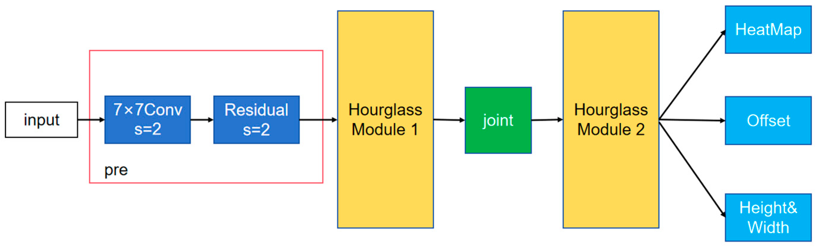
CenterNet detects an object’s position based on the center of the detection box, so it has only one large branch, which contains three small branches. The network structure diagram is shown in Figure 1. As can be seen from the graph, the input is processed by a 7 × 7 convolution with a step size of 2 and a residual error unit with a step size of 2 to compress the width and height of the image into a quarter of the original. The first hourglass convolutional neural network is followed by a joint connection to the second hourglass convolutional neural network module and a three-branch output at the head. The heatmap branch size is (W/4, H/4, C), and the offset branch size is (W/4, H/4, 2), which is used to refine the heatmap output and improve the location accuracy. The width branch size (W/4, H/4, 2) is used to predict the width and height of the key point-centric detection box. The loss function consists of the sum of the three parts of the output loss.
FCOS is not only an unanchored detector but also a one-stage convolutional neural network (a fully convolutional network, FCN). The network architecture diagram is shown in Figure 2. The backbone network is Resnet50, and the Feature Pyramid Network (FPN) generates P3, P4, and P5 on the C3, C4, and C5 outputs of the backbone network; then, on the basis of P5, we obtain P6 from a convolution layer with a convolution kernel size of 3 × 3 and a step length of 2; finally, based on P6, P7 is obtained from a convolution layer with a convolution kernel size of 3 × 3 and a step length of 2. The detection head is shared by P3–P7, which is divided into three branches: classification, regression, and IOU (center-ness), where regression and center-ness are two distinct sub-branches on the same branch. As can be seen from the diagram, each branch will first pass through the four composite modules of “convolution layer + normalization layer + activation function layer”; finally, a convolution layer with the size of 3 × 3 step is used to obtain the final prediction result. The colors blue, green, red, orange, and purple in the image represent the head, neck (PAFPN) portion, classification branch, regression branch, center-ness branch, and convolution layers in the head, respectively. For the classification branch, several score parameters of the target detection task category are predicted on each position of the prediction feature map. For the regression branch, four distance parameters are predicted on each position of the prediction feature map, i.e., the distance from the left side of the target, upper side distance, right side distance, and lower side distance; at this point, the predicted values are on the scale of the relative feature map. For the center-ness branch, one parameter center-ness is output at each location of the predicted feature map, which reflects the distance of a point on the feature map to the target center, with a range of 0 to 1. The closer the point is to the target center, the closer the output parameter value is to 1, and the farther the distance is from the target center, the closer the output parameter value is to 0.
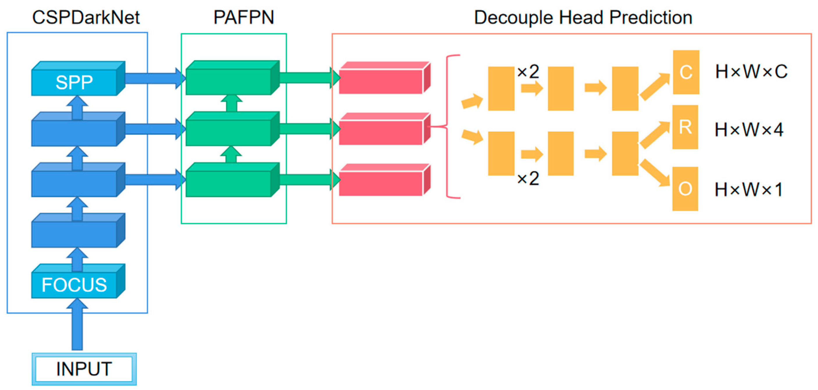
YOLOX is an improvement on YOLOV5, and its structure diagram is shown in Figure 3. Three of the key innovations are its decoupled head, the fact that it is anchor-free, and its advanced label assigning strategy (SimOTA). Previous probes were implemented using a convolution layer with a convolution core size of 1 × 1 that predicted both category scores, bounding box regression parameters, and object-ness; this approach is called a coupled detection head. The creators of YOLOX think that the coupling detector is harmful to the detection performance of the network; if it is replaced by the decoupling detector, the convergence speed of the network can be greatly improved, and the corresponding experiments can be carried out. The results show that AP can be improved by about 1.1 points by using a decoupling head. Three different branches are used for prediction classification (C), regression (R), and IOU parameters (O) in decoupling heads, but different heads are used for different prediction feature graphs in YOLOX, that is, parameters are not shared. On the surface, the decoupling detector improves the performance and convergence speed of YOLOX, but on a deeper level, it makes it possible to integrate it with the downstream detection tasks.
In the image, blue represents the backbone network, and light blue represents some special modules (FOCUS and SPP) in the base backbone model. The FOCUS structure obtains four independent feature layers by taking a value every other pixel in an image, then the four independent feature layers are stacked; at this point, the width and height information is concentrated on the channel information, and the input channel expanded four times. The SPP structure extracts features by a maximum pool of different pool sizes to improve the receptive field of the network. Green indicates the neck (Pyramid Attention Feature Pyramid Network, PAFPN) section, red indicates the head, orange indicates the convolution layer of the head, C indicates the classification branch, R indicates the regression branch, and O indicates the IOU branch. In H × W × C, C represents the number of target classes detected, 4 represents the target bounding box parameter of network prediction, and 1 represents the object-ness (IOU) parameter.
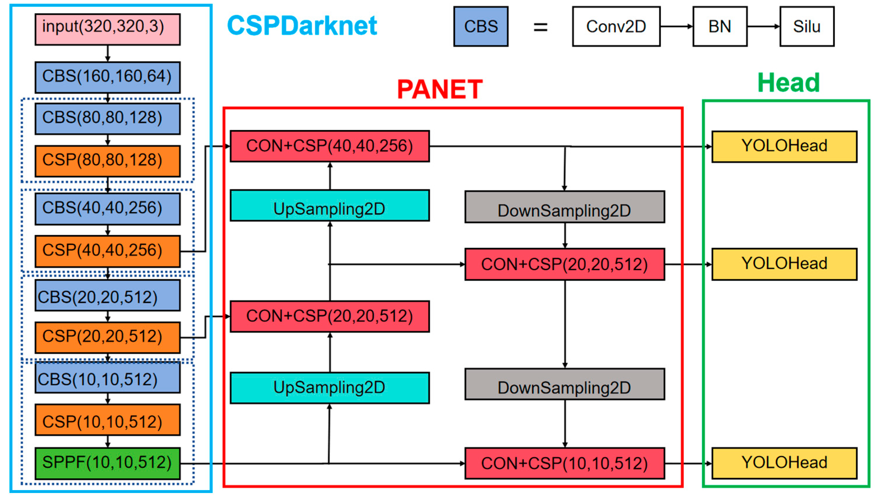
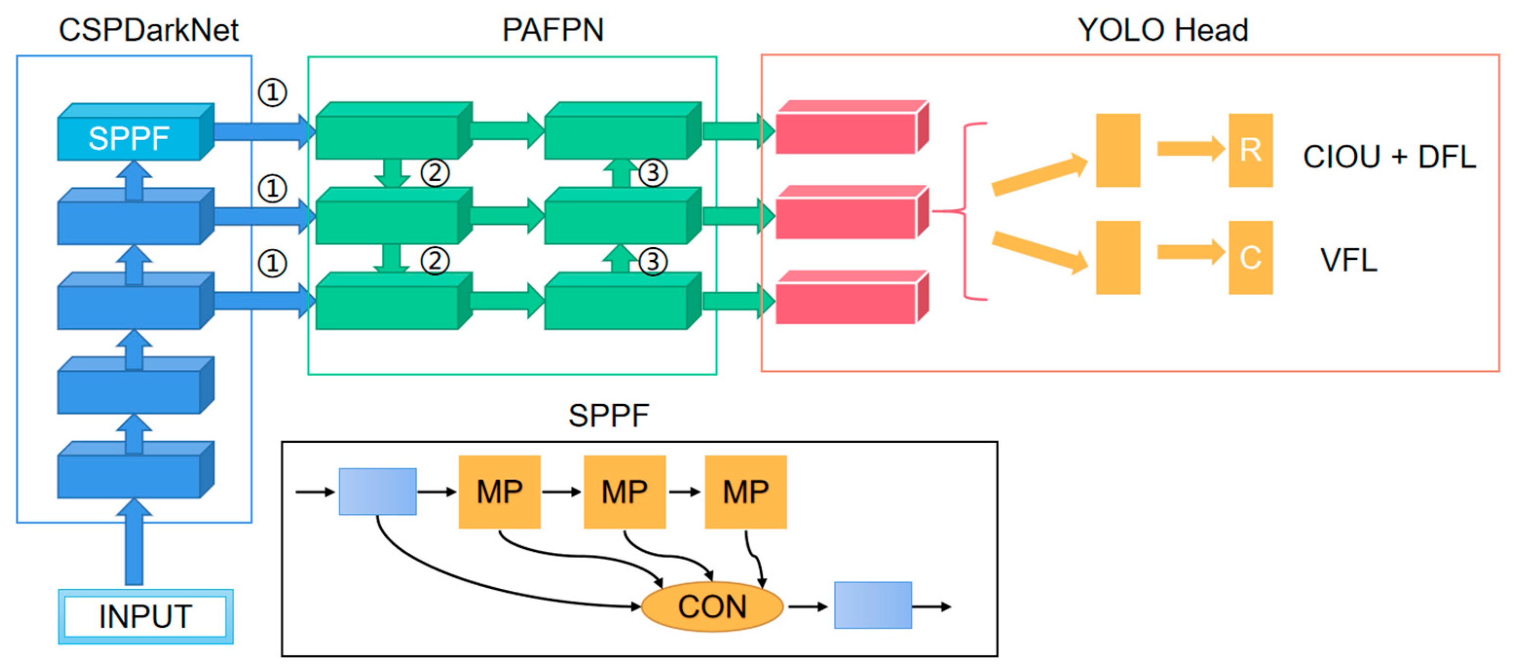
The YOLOV8 network structure and prediction method is similar to the previous YOLO series. It is divided into three parts: the backbone, FPN, and head. The structure diagram is shown in Figure 4. The backbone is the backbone feature extraction network, which extracts the feature of the input image. The extracted feature layer is the feature set of the input image. Three feature layers are selected for the next step of network construction. FPN is an enhanced feature extraction network, in which three feature layers obtained in the backbone are fused to combine different scales of feature information. Using the path aggregation network (PANET) in YOLOV8, feature fusion is realized not only by up-sampling but also by down-sampling. The head is the network’s classifier and regressor, with the backbone and FPN providing three enhanced feature layers. Each feature layer has a width, height, and number of channels, so the feature map can be regarded as a set of one feature point after another, and each feature point is regarded as an a priori point instead of an a priori frame. Each a priori point has several characteristics of the channel. The head judges the feature point, to determine whether there is an object in the a priori box on the feature point corresponding to it. The detector used by YOLOV8 is decoupled, meaning that classification and regression are not implemented in the same 1 × 1 convolution. Therefore, the work of the whole network can be summarized as follows: feature extraction, feature enhancement, and prediction of objects corresponding to an a priori box.
The backbone feature extraction network makes some optimizations to improve the detection speed: the neck structure uses a 3 × 3 convolution with a normal step size of 2; the CSP module preprocesses two convolutions instead of three convolutions; it also borrows from YOLOV7’s multi-stack architecture. That is, the number of channels of the first convolution is expanded to double the original, and then the result of the convolution is split in half on the channels, which can reduce the number of times of the first convolution and speed up the network.
In the figure, CBS refers to the “Convolution layer + batch layer + activation function layer” module. Con represents a connection operation. UpSampling2D represents the up-sampling operation, DownSampling2D represents the down-sampling operation, YOLOHead represents the detection head of the network, and the three-dimensional vector in parentheses represents the dimension shape of the feature graph of each layer. The light-blue rectangle represents the backbone of the network CSPDarknet, the red rectangle represents the PANET structure of the network neck, and the green rectangle represents the detection decoupling head of the network. 
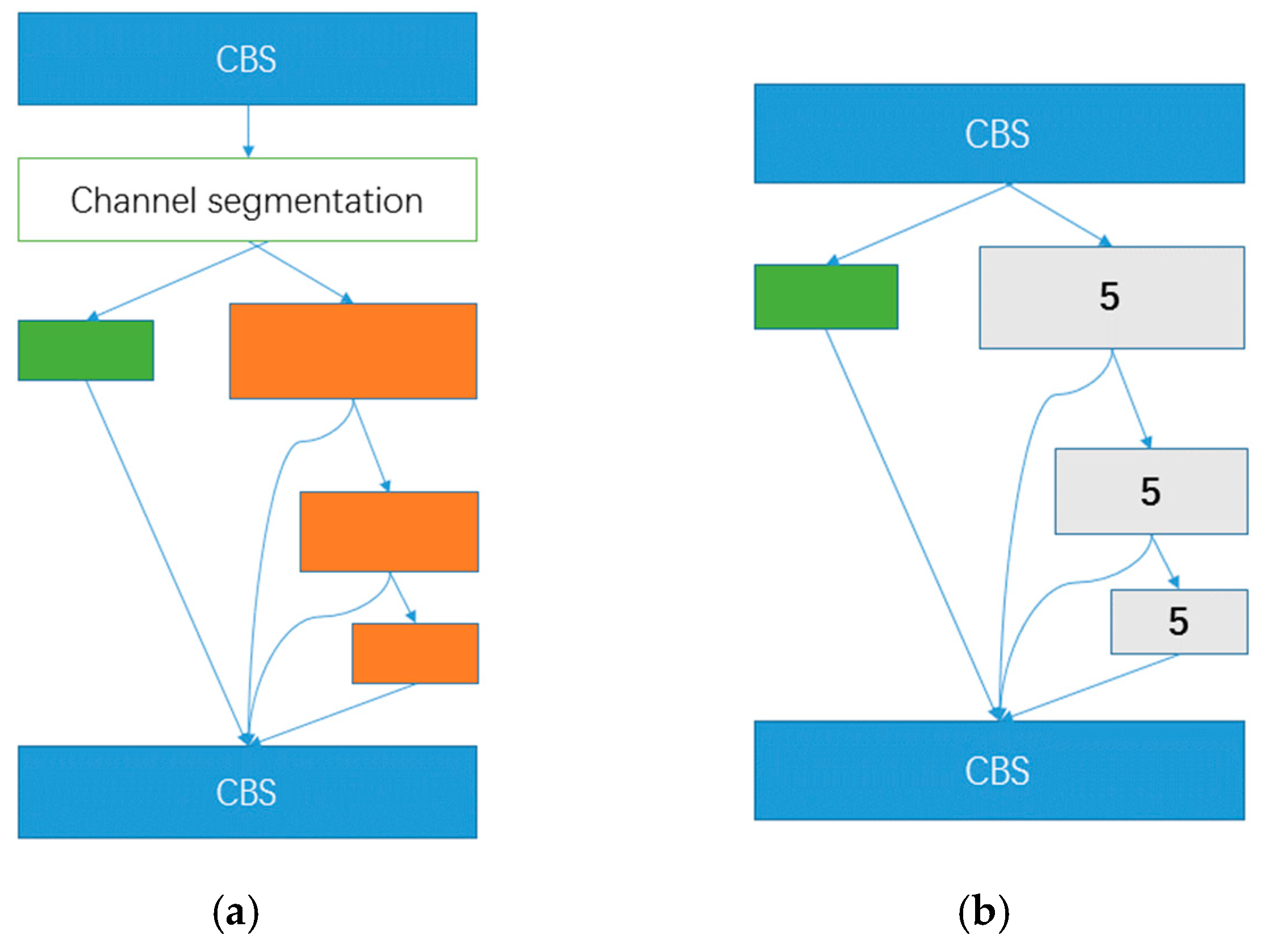
Figure 5 shows the CSP module schematic diagram (a) and the SPPF module schematic diagram (b). The orange represents a bottleneck module, while the green represents no processing. 5 represents the maximum pooling with a kernel size of 5.
The loss of YOLOV8 consists of two parts: (1) The regression part: Since YOLOV8 uses DFL for the final regression prediction, it is necessary to add DFL loss to the regression section. The regression loss for YOLOV8 consists of IOU loss versus DFL loss. The IOU loss is calculated by calculating the coincidence of the predicted box and the true box P and then using 1-p. DFL loss is calculated in a probabilistic way, so using cross-entropy, DFL classifies the regression target as a classification target; taking the upper-left corner of the real box as an example, it generally does not lie on a specific grid point, and its coordinates are not integers (the computational loss is not relative to the real graph, but to the grid graph of each feature layer). If the real box is 6.7, then it is closer to 7 and farther away from 6. Therefore, two cross-entropies can be used, that is, the prediction results with 6 cross-entropy given a lower weight, and the prediction results with 7 cross-entropy given a higher weight. (2) The category section: The cross-entropy loss is calculated as the loss component of the category part according to the category of the true frame and the category of the a priori frame. But the label is not 1 at this time, but rather calculated by the degree of coincidence, that is, by the cost function times the forecast box and the true box of the degree of coincidence divided by the true box corresponding to the maximum value.

3.2. Improved Model

The primary goal of the attention mechanism is to direct the network’s attention toward areas that require greater attention in order to achieve adaptive attention in the system. Broadly speaking, there are three types of attention mechanisms: spatial, channel, and hybrid attention mechanisms. Though location information is crucial for creating spatially selective attention maps, channel attention (e.g., SE attention) has a substantial impact on enhancing model performance. Consequently, unlike channel attention, which combines feature tensors into a single feature vector through two-dimensional global pooling, Coordinate Attention (CA), a network attention mechanism, is utilized in this paper to decompose channel attention into two one-dimensional feature coding processes that aggregate features along two spatial directions. This makes it possible to record precise location information along one spatial direction while capturing remote dependencies along another. After that, the feature map is encoded into two attention maps: one that is location-sensitive and another that is direction-aware. These attention maps can be applied complementarily to the input feature map to improve the representation of objects of interest. Figure 6 below displays the CA block schematic diagram.
The attention mechanism is a plug-and-play module that can be positioned in a reinforced feature extraction network, behind any feature layer, or behind a backbone network. This paper applies the attention mechanism to the enhanced feature extraction network because the pre-training weights of the network cannot be used when placed on the backbone. At this point, attention modules can be inserted into the network at three different positions: after the reinforcement feature layer (①), after up-sampling and before the connection layer (②), and after down-sampling and before the connection layer (③). The specific insertion network structure diagram is displayed in Figure 7 below.
In the image, red denotes the head, orange in the red anchor indicates the convolution layers in the head, blue represents the backbone, light blue indicates some special module (SPPF) in the base backbone model, green represents the neck (PAFPN) portion, and R stands for regression branch. The black anchor displays the SPPF detail; the graduated blue indicates the “Batch Normalization + Leaky Relu model + Convolution”; MP stands for Maxpool layer; and CON stands for Concat operate.

4. Experiments

All the environment configurations used in this experiment are shown in Table 1 below.

4.1. Wind Turbine Blade Surface Defect Detection

It is worthwhile to concentrate on wind power generation equipment because wind energy is a renewable green energy source with promising future growth. Fan blades are a crucial component of wind turbines and are expensive to manufacture and install. The normal operation and financial benefits of wind power systems are directly impacted by the health and lifespan of these blades. Fan blades are more likely to have large or small defects during the molding process because of their complex manufacturing process. Additionally, because fans operate in harsh environments, external factors may also cause surface damage and defects during the working process. Studying the corresponding surface defect detection of fan blades is therefore crucial. A tiny fan blade surface defect detection dataset, divided into four categories (normal, depainting, oil spill, and flaw), was created by using an unmanned aerial vehicle to take pictures of real fan blades in a wind farm. The size of the original captured photo, measuring 3936 × 2624 pixels, exceeds the input size of the target detection network. Consequently, 480 images are ultimately obtained by random flipping and cropping, mixup, mosaic data enhancement, and the selection of 120 original images that are cropped to 300 × 300 size images. A total of 120 images are obtained for each category. The dataset is then split into three groups: a training set of 388 images, a validation set of 44 images, and a test set of 48 images. There were 313 depainting defects, 222 flaw defects, 153 normal images, and 116 oil spill defects. The reason why the number of defects is different is that after data enhancement, the defect parts of some images will be clipped, and the number and type of defects of the same image are not unique. The pre-processed dataset will increase the complexity of the data due to the addition of disturbance factors, which makes the data in the training process of the network model more diverse; even if the dataset is small, you can still obtain better results.
A few of the sample pictures are displayed in Figure 8 below. The original image (a), the cropped and randomly reversed image (b), the mixup operation image (c), and the mosaic operation image (d) are arranged from left to right.

4.2. Training Parameters and Experimental Metrics

The input image size is 320 × 320. We used a two-stage training method. During the freezing stage, the backbone network remains unchanged, and only the other parts are fine-tuned. And during the unfreezing stage, all parts of the model will be changed to better adapt to the detection needs of this dataset. The Adam optimizer and cosine annealing learning rate reduction algorithm are used in the training process. The CenterNet’s learning rate is 5 × 10⁻⁴, and the momentum is 0.9; the FCOS’s learning rate is 3 × 10⁻⁴, and the momentum is 0.9; YOLOX-S has a learning rate of 1 × 10⁻² with a momentum of 0.937, the mosaic-prob is 0.5, the mixup-prob is 0.5, and it closed early; and YOLOV8-S has a learning rate of 1 × 10⁻³ with a momentum of 0.937.
We usually use parameters and FLOPs to measure the lightweight level and the algorithm complexity. Latency is the time that the network takes to predict an image. Frames per second (FPS) is the reciprocal of the latency. Precision is the proportion of true positive samples over all the positive samples that the classifier predicted. Recall is the proportion of true positive samples over all real positive samples. The average precision (AP) is the area under the precision–recall curve, and mAP is the mean of all APs of defect types.

4.3. Results and Analysis

We compared the parameter sizes of CenterNet, FCOS, YOLOX-S, and YOLOV8-S with FLOPs in Table 2. It can be seen that CenterNet and FCOS have more complex structures, and their parameter sizes are higher than the other two network models. The FLOPs values are also relatively large. The other two models not only have small parameter quantities but also have lower FLOPs values, which consume fewer computing resources, providing a greater possibility for the deployment of real-time detection applications.
The detection results for each type are detailed in Table 3 below. From the table, it can be seen that CenterNet has the lowest mAP, with only the paint stripping type detected, and the remaining three types are undetectable and therefore are not recommended for practical applications. FCOS has the highest detection accuracy (85.24%), but it has a slow detection speed of 1.67 with high latency. And YOLOX, despite having the highest FPS (10.94), has a low average mean accuracy of 57.51%. YOLOV8-S is the best detector in terms of detection performance among all the unanchored frame detectors compared in this paper. It not only has a high detection accuracy (79.55%) but also has a high FPS (9.52) and low latency (0.1052). We will use this model for subsequent studies on surface defect detection on wind turbine blades.
The relationship between the FLOPs and mAP of the comparison detectors is shown in Figure 9, which shows the performance of the four anchorless frame detectors more clearly, where the horizontal axis is the amount of floating-point operations and the closer to the left side of the model, the more lightweight it is; the vertical axis is the average accuracy, where the closer to the top of the model, the higher the accuracy of the detection; the size of the bubble represents the number of frames transmitted per second, where the bigger the bubble, the faster the detection of the model, and the closer to the top left and the bigger the bubble, the stronger the combined detection performance of the network model. From the figure, it is known that YOLOV8 has the best performance.
The optimal number of iterations to be used for the next experiments was determined by the accuracy of the model evaluated on the validation set during training. A total of 200 epochs were trained above and evaluated every 20 epochs on the validation set. The evaluation mAP is shown in Figure 10 below.
As shown in the figure, the network model reaches its maximum at 160 and 200 epochs, so we compare the results for different epochs of training in Table 4 below. mAP is similar, but the FPS is improved by 1. Therefore, we choose 200 as the final number of iterations. We still use a batch size of 32. The first 50 epochs are used as the freezing training phase, and the last 150 epochs are used as the unfreezing training phase. In the next experiments, we use the same evaluation metrics as above.
The changes in detection performance when comparing CAs added at different locations in the network model are shown in Table 5 below, from which it can be seen that among all the compared methods, the model has the optimal detection accuracy when the attention module is inserted in the backbone, up-sampling, and down-sampling parts (BCA + UCA + DCA), with an average mean accuracy of 84.78%, which is a 5.23% increase compared to the original model, and the number of frames transmitted per second is 8.49, which is a 1.03 decrease. The average mean accuracy is 84.78%, which is 5.23% higher than the original model, while the number of frames transmitted per second is 8.49, which is 1.03 lower, and the average mean accuracy and the number of frames transmitted per second when the attention module is inserted into both the backbone and the down-sampling part (BCA + DCA) are 84.54% and 9.16, which are 4.99% and 0.36 lower than the original model, respectively. The BCA + DCA model is the most optimal model in the overall view.

4.4. Further Experiments

4.4.1. Comparison of NEU Dataset

Six different types of defects were gathered by Northeastern University’s (NEU) surface detection datasets for hot-rolled steel strip steel: crazing (Cr), inclusion (In), patches (Pa), pitted surface (PS), rolled-in surface (RS), and scratches (Sc). There were 300 photos for each defect, for a total of 1800 grayscale images. Additionally, every image has a resolution of 200 × 200 pixels. The accompanying Figure 11 provides a few sample pictures.
The results of different CA modules inserted into the model location on the NEU dataset are compared as shown in Table 6 below. From the table, it can be seen that the BCA + DCA model has the highest detection accuracy, which is improved by 1.06% compared to the original model, while the BCA + UCA + DCA model, which has the best performance in terms of accuracy rate on the wind turbine blade surface defect detection dataset, performs poorly on the NEU dataset, which is only improved by 0.32%. It is presumed that the difference in the original images causes this phenomenon to occur, as the wind turbine dataset is a three-channel color image, while the NEU dataset is a single-channel grayscale image, which leads to a bias in the integration of information between the two by the channel attention module.

4.4.2. Comparison of Grayscale Channel

According to the above conjecture, the ablation experiment was carried out, and the original three-channel color image was transformed into a single-channel gray image; the results are shown in Table 7. The mAP of the BCA + DCA insertion mode was 85.15%, which was 2.82% higher than that of the BCA + UCA + DCA insertion mode, and the FPS decreased only 0.5% in the gray image defect detection dataset of fan blades. When changing the dataset of fan blade surface defect detection to the gray image dataset, it is the same as the dataset of hot-rolled strip surface defect detection, and the YOLOV8 model with the BCA + DCA insertion mode has the best detection performance.
The results of the grayscale leaf image contrast were visualized with their thermograms shown in Figure 12, with (a) representing the BCA + DCA model and (b) representing the BCA + UCA + DCA model. The diagram shows that the BCA + DCA insertion model is more focused on the thermal range of the defect location, that is, the network is more sensitive to the defect location.

4.4.3. Comparison of Source Domain Dataset

Using transfer learning ideas (fine-tuning) can alleviate the overfitting problem caused by applying large models to small datasets, considering that transfer learning is sensitive to the similarity between the distribution of source domain data and target domain data, the model detection performance of transferring to the fan blade dataset was compared between the COCO dataset and the Northeastern University hot-rolled strip dataset. The results are shown in Table 8, where 200_COCO represents the result of training 200 epochs with the COCO dataset as the source domain dataset, and 200_NEU represents the result of training 200 epochs with the NEU dataset as the source domain dataset.
As can be seen from the table above, the overall migration is not as good, although intuitively the data distribution of the NEU dataset is more similar to the wind turbine blade surface defect dataset we constructed. However, there is a better performance in the detection of the paint stripping and oil staining categories, which is presumed to be due to the irregular shapes of these two defect types, which are closer to the strip surface defect types, while the normal type has a more rounded, elliptical shape, and the crack type is characterized by elongated and inconspicuous features, which is a big difference in the shape characteristics of the defect types in the strip dataset, which leads to a less than optimal effect of the migration learning. At the same time, since we only trained the model on the NEU data for 200 rounds, and the COCO dataset was trained for far more rounds, this means that our pre-trained model may not have learned the more robust and generalized features well, but at this point, our average mean accuracy is only two percentage points less. If we had used a larger number of rounds on the NEU dataset for pre-training, the results would have been different, which is worth exploring further.

5. Discussion and Conclusions

This paper applies the anchor-free detection algorithm to the field of component surface defect detection. Based on the real fan images captured by UAV, a small fan blade surface defect detection dataset is established, and the detection performance of four existing non-anchor frame target detectors is compared. Finally, it was determined that YOLOV8 had the best comprehensive performance. Next, a large number of experiments were conducted to compare the effect of the attention module on the detection effect of the target detector when inserting different positions of the model; the results show that the model has the best detection precision when the attention module is inserted in the backbone, the upper, and the lower sampling parts; the average precision reaches 84.78%, which is 5.23% higher than the original model; and the number of frames per second was 8.49, down 1.03. When the attention module was inserted in the backbone and the lower sampling, the average precision and the number of frames per second were 84.54% and 9.16, respectively, which were improved by 4.99% and decreased by 0.36 compared with the original model. The performance of the former is better than latter, and the performance of this method is also the best on the dataset of hot strip surface detection in Northeastern University.
Following this research, we will determine whether the sample matching strategy—which could be examined further—is the primary distinction between the so-called anchor-based and anchor-free models. In addition, we will use this dataset for pixel-level surface defect detection and segmentation tasks in order to obtain more accurate defect sizes, taking into account the fusion of adversarial generation networks to generate a fan blade surface defect detection dataset with a more realistic and natural distribution for research work.

Author Contributions

Writing—original draft preparation, J.L. (Jiaxue Liu); project administration, C.Z.; modifications, J.L. (Jianjun Li). All authors have read and agreed to the published version of the manuscript.

Funding

This work was supported by the National Natural Science of China (Grant No. 52365014), Central Government Guiding Local Science and Technology Development Fund Project (Grant No. 2022ZY0221), Science and Technology Plan Projects of Inner Mongolia Autonomous Region (Grant No. 2023YFSW0003), and Fundamental Research Funds for Inner Mongolia University of Science & Technology (Inner Mongolia Autonomous Region Key Laboratory of Intelligent Diagnosis and Control of electromechanical systems).

Data Availability Statement

The dataset of hot-rolled steel strip steel surface defects was obtained from the Northeastern University. The dataset of wind blade surface defects is unavailable due to privacy or ethical restrictions.

Conflicts of Interest

The authors declare no conflicts of interest.

References

  1. Girshick, R.; Donahue, J.; Darrell, T.; Malik, J. Rich feature hierarchies for accurate object detection and semantic segmentation. In Proceedings of the IEEE Conference on Computer Vision and Pattern Recognition, Columbus, OH, USA, 23–28 June 2014; pp. 580–587. [Google Scholar]
  2. He, K.; Zhang, X.; Ren, S.; Sun, J. Spatial pyramid pooling in deep convolutional networks for visual recognition. IEEE Trans. Pattern Anal. Mach. Intell. 2015, 37, 1904–1916. [Google Scholar] [CrossRef] [PubMed]
  3. Girshick, R. Fast r-cnn. In Proceedings of the IEEE International Conference on Computer Vision, Santiago, Chile, 7–13 December 2015; pp. 1440–1448. [Google Scholar]
  4. Ren, S.; He, K.; Girshick, R.; Sun, J. Faster r-cnn: Towards real-time object detection with region proposal networks. arXiv 2015, arXiv:1506.01497. [Google Scholar] [CrossRef] [PubMed]
  5. Redmon, J.; Divvala, S.; Girshick, R.; Farhadi, A. You only look once: Unified, real-time object detection. In Proceedings of the IEEE Conference on Computer Vision and Pattern Recognition, Las Vegas, NV, USA, 27–30 June 2016; pp. 779–788. [Google Scholar]
  6. Liu, W.; Anguelov, D.; Erhan, D.; Szegedy, C.; Reed, S.; Fu, C.Y.; Berg, A.C. Ssd: Single shot multibox detector. In Proceedings of the Computer Vision–ECCV 2016: 14th European Conference, Amsterdam, The Netherlands, 11–14 October 2016; Springer International Publishing: Cham, Switzerland, 2016; pp. 21–37. [Google Scholar]
  7. Liu, L.; Ouyang, W.; Wang, X.; Fieguth, P.; Chen, J.; Liu, X.; Pietikäinen, M. Deep learning for generic object detection: A survey. Int. J. Comput. Vis. 2020, 128, 261–318. [Google Scholar] [CrossRef]
  8. Cai, Y.; Li, H.; Yuan, G.; Niu, W.; Li, Y.; Tang, X.; Ren, B.; Wang, Y. Yolobile: Real-time object detection on mobile devices via compression-compilation co-design. In Proceedings of the AAAI Conference on Artificial Intelligence, Online, 2–9 February 2021; Volume 35, pp. 955–963. [Google Scholar]
  9. Ristić-Durrant, D.; Franke, M.; Michels, K. A review of vision-based on-board obstacle detection and distance estimation in railways. Sensors 2021, 21, 3452. [Google Scholar] [CrossRef] [PubMed]
  10. Wang, T.; Yang, F.; Tsui, K.L. Real-time detection of railway track component via one-stage deep learning networks. Sensors 2020, 20, 4325. [Google Scholar] [CrossRef]
  11. Jothiaruna, N. SSDMNV2-FPN: A cardiac disorder classification from 12 lead ECG images using deep neural network. Microprocess. Microsyst. 2022, 93, 104627. [Google Scholar]
  12. Akshatha, K.R.; Karunakar, A.K.; Shenoy, S.B.; Pai, A.K.; Nagaraj, N.H.; Rohatgi, S.S. Human Detection in Aerial Thermal Images Using Faster R-CNN and SSD Algorithms. Electronics 2022, 11, 1151. [Google Scholar] [CrossRef]
  13. Wang, Z.; Lian, J.; Song, C.; Zhang, Z.; Zheng, W.; Yue, S.; Ji, S. SAS: Painting Detection and Recognition via Smart Art System With Mobile Devices. IEEE Access 2019, 7, 135563–135572. [Google Scholar] [CrossRef]
  14. Arcos-García, Á.; Alvarez-Garcia, J.A.; Soria-Morillo, L.M. Evaluation of deep neural networks for traffic sign detection systems. Neurocomputing 2018, 316, 332–344. [Google Scholar] [CrossRef]
  15. El-Bana, S.; Al-Kabbany, A.; Sharkas, M. A two-stage framework for automated malignant pulmonary nodule detection in CT scans. Diagnostics 2020, 10, 131. [Google Scholar] [CrossRef]
  16. Huang, L.; Yang, Y.; Deng, Y.; Yu, Y. DenseBox: Unifying Landmark Localization with End to End Object Detection. arXiv 2015, arXiv:1509.04874. [Google Scholar]
  17. Law, H.; Deng, J. Cornernet: Detecting objects as paired keypoints. In Proceedings of the European Conference on Computer Vision (ECCV), Munich, Germany, 8–14 September 2018; pp. 734–750. [Google Scholar]
  18. Zhou, X.; Zhuo, J.; Krahenbuhl, P. Bottom-up object detection by grouping extreme and center points. In Proceedings of the IEEE/CVF Conference on Computer Vision and Pattern Recognition, Long Beach, CA, USA, 15–20 June 2019; pp. 850–859. [Google Scholar]
  19. Duan, K.; Bai, S.; Xie, L.; Qi, H.; Huang, Q.; Tian, Q. Centernet: Keypoint triplets for object detection. In Proceedings of the IEEE/CVF International Conference on Computer Vision, Seoul, Republic of Korea, 27 October–2 November 2019; pp. 6569–6578. [Google Scholar]
  20. Tian, Z.; Shen, C.; Chen, H.; He, T. FCOS: A simple and strong anchor-free object detector. IEEE Trans. Pattern Anal. Mach. Intell. 2020, 44, 1922–1933. [Google Scholar] [CrossRef]
  21. Kong, T.; Sun, F.; Liu, H.; Jiang, Y.; Li, L.; Shi, J. FoveaBox: Beyound Anchor-Based Object Detection. IEEE Trans. Image Process. 2020, 29, 7389–7398. [Google Scholar] [CrossRef]
  22. Zheng, G.; Liu, S.; Wang, F.; Li, Z.; Sun, J. YOLOX: Exceeding YOLO Series in 2021. arXiv 2021, arXiv:2107.08430. [Google Scholar]
  23. Available online: https://github.com/ultralytics/ultralytics.git (accessed on 20 October 2024).
  24. Wang, Y.; Wang, H.; Xin, Z. Efficient detection model of steel strip surface defects based on YOLO-V7. IEEE Access 2022, 10, 133936–133944. [Google Scholar] [CrossRef]
  25. Aboah, A.; Wang, B.; Bagci, U.; Adu-Gyamfi, Y. Real-time multi-class helmet violation detection using few-shot data sampling technique and yolov8. In Proceedings of the IEEE/CVF Conference on Computer Vision and Pattern Recognition Workshops (CVPRW), Vancouver, BC, Canada, 17–24 June 2023; pp. 5349–5357. [Google Scholar]
  26. Lou, H.; Duan, X.; Guo, J.; Liu, H.; Gu, J.; Bi, L.; Chen, H. DC-YOLOv8: Small-Size Object Detection Algorithm Based on Camera Sensor. Electronics 2023, 12, 2323. [Google Scholar] [CrossRef]
  27. Gao, Y.; Hou, R.; Gao, Q.; Hou, Y. A Fast and Accurate Few-Shot Detector for Objects with Fewer Pixels in Drone Image. Electronics 2021, 10, 783. [Google Scholar] [CrossRef]
  28. Chen, C.; Fu, R.; Ai, X.; Huang, C.; Cong, L.; Li, X.; Jiang, J.; Pei, Q. An Integrated Method for River Water Level Recognition from Surveillance Images Using Convolution Neural Networks. Remote Sens. 2022, 14, 6023. [Google Scholar] [CrossRef]
  29. Lei, Y.; Wang, T.; Roper, J.; Jani, A.B.; Patel, S.A.; Curran, W.J.; Patel, P.; Liu, T.; Yang, X. Male pelvic multi-organ segmentation on transrectal ultrasound using anchor-free mask CNN. Med. Phys. 2021, 48, 3055–3064. [Google Scholar] [CrossRef]
  30. Wang, Q.; Wang, Y.; Zhou, Y.; Wang, J.; Jiang, W.; Zhang, X. SSPSNet: A single shot panoptic segmentation network for accurate scene parsing. Neural Comput. Appl. 2022, 34, 677–688. [Google Scholar] [CrossRef]
  31. Chen, Y.; Ding, Y.; Zhao, F.; Zhang, E.; Wu, Z.; Shao, L. Surface Defect Detection Methods for Industrial Products: A Review. Appl. Sci. 2021, 11, 7657. [Google Scholar] [CrossRef]
  32. Yang, J.; Li, S.; Wang, Z.; Dong, H.; Wang, J.; Tang, S. Using Deep Learning to Detect Defects in Manufacturing: A Comprehensive Survey and Current Challenges. Materials 2020, 13, 5755. [Google Scholar] [CrossRef] [PubMed]
  33. Wang, C.; Xiao, Z. Lychee surface defect detection based on deep convolutional neural networks with gan-based data augmentation. Agronomy 2021, 11, 1500. [Google Scholar] [CrossRef]
  34. Li, G.; Zhao, S.; Zhou, M.; Li, M.; Shao, R.; Zhang, Z.; Han, D. YOLO-RFF: An Industrial Defect Detection Method Based on Expanded Field of Feeling and Feature Fusion. Electronics 2022, 11, 4211. [Google Scholar] [CrossRef]
  35. Li, Y.; Xu, J. Electronic product surface defect detection based on a MSSD network. In Proceedings of the 2020 IEEE 4th Information Technology, Networking, Electronic and Automation Control Conference (ITNEC), Chongqing, China, 12–14 June 2020; IEEE: Piscataway, NJ, USA, 2020; Volume 1, pp. 773–777. [Google Scholar]
  36. Huang, L.; Gong, A. Surface Defect Detection for No-Service Rails With Skeleton-Aware Accurate and Fast Network. IEEE Trans. Ind. Inform. 2024, 20, 4571–4581. [Google Scholar] [CrossRef]
  37. Qian, X.; Wang, X.; Yang, S.; Lei, J. LFF-YOLO: A YOLO Algorithm With Lightweight Feature Fusion Network for Multi-Scale Defect Detection. IEEE Access 2022, 10, 130339–130349. [Google Scholar] [CrossRef]
  38. Bouguettaya, A.; Mentouri, Z.; Zarzour, H. Deep ensemble Transfer Learning-based approach for classifying hot-rolled steel strips surface defects. Int. J. Adv. Manuf. Technol. 2023, 125, 5313–5322. [Google Scholar] [CrossRef]
  39. Zhao, W.; Chen, F.; Huang, H.; Li, D.; Cheng, W. A New Steel Defect Detection Algorithm Based on Deep Learning. Comput. Intell. Neurosci. 2021, 2021, 5592878. [Google Scholar] [CrossRef]
  40. Yu, Y.; Chan, S.; Tang, T.; Zhou, X.; Yao, Y.; Zhang, H. Surface Defect Detection of Hot Rolled Steel Based on Attention Mechanism and Dilated Convolution for Industrial Robots. Electronics 2023, 12, 1856. [Google Scholar] [CrossRef]
  41. Shao, Y.; Fan, S.; Zhao, Q.; Zhang, L.; Sun, H. Surface Defect Detection of Aluminum Profiles Based on Multiscale and Self-Attention Mechanisms. Sensors 2024, 24, 2914. [Google Scholar] [CrossRef]
Figure 1. Diagram of the CenterNet model structure.
Processes 12 02817 g001
Figure 2. Diagram of the FCOS model structure.
Processes 12 02817 g002
Figure 3. YOLOX structure diagram.
Processes 12 02817 g003
Figure 4. YOLOV8 structure diagram.
Processes 12 02817 g004
Figure 5. The CSP module schematic diagram (a) and the SPPF module schematic diagram (b).
Processes 12 02817 g005
Figure 6. The structure of CA block.
Processes 12 02817 g006
Figure 7. Improved YOLOV8 structural diagram with various attention module (CA block) insertion techniques.
Processes 12 02817 g007
Figure 8. Example images of the wind turbine blade surface defect detection dataset.
Processes 12 02817 g008
Figure 9. Plot of model FLOPs–mAP relationship.
Processes 12 02817 g009
Figure 10. Validation set evaluation accuracy plot.
Processes 12 02817 g010
Figure 11. Some images of the NEU datasets. They, respectively, represent crazing (a), inclusion (b), patches (c), pitted surface (d), rolled-in surface (e), and scratches (f). The original image size is 200 × 200, with (a) being 200 × 200 and a scale of 1:1, (b) being 208 × 208 and a scale of 1.04:1, (c) being 194 × 194 and a scale of 0.97:1, (d) being 200 × 200 and a scale of 1:1, (e) being 192 × 192 and a scale of 0.96:1, and (f) being 200 × 200 and a scale of 1:1.
Processes 12 02817 g011
Figure 12. The results of the grayscale leaf image. BCA + DCA model (a) and BCA + UCA + DCA model (b).
Processes 12 02817 g012
Table 1. Training and testing environment configuration.
ProjectConfiguration
Operating systemWindows10 Professional Edition
CPUIntel(R)Xeon(R)CPU E5-2620V4@2.10 GHZ ×2
GPUNVIDIA TITAN V ×2
GPU acceleratorCUDA11.6.1, CUDNN8.5.0.96
RAM64 GB
LanguagePython 3.8.13
Framework environmenttorch 1.11.0, torchvision 0.12.0
Compiler IDESpyder 5.4.3
Table 2. Parameter comparison table.
Params (M)FLOPs (G)
CenterNet32.66527.417
FCOS32.12340.362
YOLOX-S8.946.692
YOLOV8-S11.1387.164
Table 3. Detailed accuracy of detection of various types of defects.
DepaintingFlawNormalOil SpillmAP (%)FPS (CPU)Latency (s)
CenterNet33.460008.36--
FCOS95.4696.3689.4759.6585.241.67350.5975
YOLOX52.2651.9382.8143.0657.5110.94450.0916
YOLOV891.3983.4886.8656.4879.559.51610.1052
Table 4. Table of results from different training epochs.
DepaintingFlawNormalOil SpillmAP (%)FPS (CPU)
160_COCO85.2785.5387.7158.7379.318.2267
200_COCO91.3983.4886.8656.4879.559.5161
Table 5. Comparison table of results of different CA module insertion methods (wind turbine blade surface defects inspection dataset).
BCAUCADCAmAP (%)FPSLatency (s)
79.559.51610.1052
79.649.39190.1065
80.488.09990.1239
84.549.15990.1092
84.788.49300.1180
76.498.19920.1992
80.948.24550.1219
78.828.31350.1207
Table 6. Comparison table of results of different CA module insertion methods (NEU dataset).
BCAUCADCACrInPaPSRSScmAP (%)FPS
39.0983.3993.2492.862.3497.3878.047.7725
41.3483.394.1291.4366.1397.3878.957.6174
36.2685.9692.8592.463.1795.8977.767.4899
36.9385.3993.2590.0471.2596.8279.17.5450
38.5588.1494.589.7962.5696.6178.367.2153
Table 7. Comparison table of the results of the two insertion methods (grayscale fan blade surface defect detection dataset).
DepaintingFlawNormalOil SpillmAP (%)FPS
BCA + DCA89.1983.8489.4778.185.157.1283
BCA + UCA + DCA89.7488.0984.2167.2882.337.6401
Table 8. Table of results from different source domain data.
DepaintingFlawNormalOil SpillmAP (%)FPS
200_COCO91.3983.4886.8656.4879.559.5161
200_NEU89.0878.4983.956.4877.228.7717
Disclaimer/Publisher’s Note: The statements, opinions and data contained in all publications are solely those of the individual author(s) and contributor(s) and not of MDPI and/or the editor(s). MDPI and/or the editor(s) disclaim responsibility for any injury to people or property resulting from any ideas, methods, instructions or products referred to in the content.

