Offshore Wind Farm Generation Simulation and Capacity Value Evaluation Considering Resonance Zone Control

Abstract

Offshore wind is a promising renewable energy generation technology and is arousing great attention in regards to pursuing carbon neutrality targets. Accurately simulating offshore wind generation can help to better optimize its operation and planning. It is also a concern that mechanical resonance is a threat to the wind turbines’ lifespan. In this paper, the time-series simulation of offshore wind generation with consideration of resonance zone (RZ) control is investigated. The output model for multiple wind farms with different spatial correlations is proposed. Additionally, the capacity value (CV) of the joint wind farms is also evaluated through a reliability-based model. The case study illustrates the offshore wind power output simulation and CV results under different farm correlation scenarios and RZ control strategies. It is shown that strong spatial correlation brings great synchronicity in wind farms’ output and results in a lower CV. The RZ control in wind simulation is validated and proven to have a marginal impact on the total output when multiple wind farms are evaluated together.

1. Introduction

Under the increasing carbon neutrality targets, developing offshore wind power in coastal regions is becoming a promising pathway. Offshore wind farms are currently widely deployed in regions such as the United Kingdom, Europe, and China [1]. Compared to onshore wind power, offshore wind has several advantages, including higher utilization hours and more stable power output. However, as the penetration of offshore wind continues to increase, optimizing the development pathways for offshore wind farms has become a significant challenge. One of the key prerequisites for addressing this challenge is to accurately simulate offshore wind power output and provide a reasonable assessment of its output characteristics.

There have been numerous studies focusing on the modeling of wind farms. Firstly, in terms of wind speed simulation, the existing research has explored various modeling methods. For instance, the long-term wind speed was widely modeled using the Weibull distribution [2], while the short-term wind speeds can be assumed to conform to a Gaussian process model [3]. Stochastic differential equations have been adopted to simulate the time-series wind speed across multiple wind farms [4]. Abdelaziz et al. [5] explored various probability distributions to fit the wind gust data and further investigated the cost return years of offshore wind farms. To accurately model the offshore wind farms’ operation in extreme events, a series of full-set, three-dimensional meteorology simulations have been conducted to figure out the empirical correction ratio and scale factor of wind speed profiles [6]. Secondly, in terms of the wind power output simulation, a book by Mathew [7] has fundamentally analyzed the modeling of wind energy conversion systems. The power generation curve of a wind turbine has been explored in various fitting equations, such as the cubic function [8]. To model the uncertainty of wind power, a method based on vine copula has shown a better result than the results from Monte Carlo simulation [9]. Considering the power decay associated with the wake effect, Feijóo and Villanueva proposed a four-parameter model for predicting wind farm power curves [10] and Wu et al. optimized the offshore wind farm operation and wind turbine layout [11]. Thirdly, in terms of the economic meaning of offshore wind farms, the life-cycle cost analysis for offshore wind farms has also been explored by investigating the feasibility of transmitting wind energy through submarine cables [12]. Wind power variability also impacts electricity market prices and loads [13], which draws great attention to effective wind power output simulation.

In addition, due to its relatively stable output, offshore wind power can contribute to the generation adequacy. Given the scale effect of offshore wind farms, it is crucial to properly assess the firm capacity of offshore wind to support the system’s load, which serves as a key index for its output characteristics. An IEEE taskforce has investigated various definitions and solving methods for the capacity value (CV) and capacity credit (CC) of wind power, providing insights into its contribution to system adequacy [14]. This taskforce has recommended the probabilistic approach based on the reliability metrics from the distribution of the thermal units’ available capacity [15]. In recent research, an analytical method demonstrated that the CV of a wind farm could be expressed by a linear combination of the chronological power output [16]. Besides the analytical method, NREL has proposed an 8760-based model that requires the load and net-load duration curve [17]. How multiple offshore wind farms can contribute to the generation adequacy of the system should be investigated, along with how the RZ control can affect these contributions.

In empirical operation, offshore wind turbines usually face complex environmental conditions, including exposure to external dynamic excitations such as winds and waves. Resonance can occur when the rotor, operating at either the rotational speed (1P) or the blade passing frequency (3P), corresponds to the first tower mode frequency. This resonance will cause fatigue and damage on the turbine’s components and shorten its lifespan [18]. Studies have explored various control techniques, such as damping control [19] and speed exclusion control [20], to actively mitigate resonance. It is well acknowledged that there are connections between power generation control and structural vibration mitigation of a wind turbine [21]. From resonance control to the offshore wind generation characteristics, the turbine’s resonance zone (RZ) control can be reflected in the power output function. However, there is no research on wind power output functions that take the RZ control into consideration.

In the existing literature, significant progress has been made in wind speed and wind power output modeling that accounts for both uncertainty and economic performance. However, the integration of spatiotemporal correlation and the wind power output function into offshore wind farm simulations is still in its early stages. There are also various studies on the calculation methods of wind farm’s CV. Nevertheless, the specific CV of offshore wind farms considering the spatiotemporal characteristics has not yet been discussed. In the domains of structure and control, the resonance of wind turbines has been thoroughly analyzed. As for the offshore wind power output simulations, it is essential to account for the effects of RZ control on the overall power output.

Regarding the above research gaps, this paper proposes the idea of simulating offshore wind farms’ output considering the RZ control. This method takes into account the spatiotemporal correlation among multiple offshore wind farms and applies it to the CV assessment of offshore wind farms. The contributions of this paper are two-fold, as follows.

(1)

An offshore wind generation simulation framework considering RZ control is proposed. The time-series wind speed is simulated based on a stochastic differential equation (SDE). The RZ control is innovatively modeled into the wind output function through a hysteresis mechanism.

(2)

A CV assessment model on offshore wind farms is proposed. The impacts from spatiotemporal correlation among various offshore wind farms on the wind output simulation and CV evaluation are then discussed in a case study.

The rest of this paper is organized as follows: In Section 2, the offshore wind power simulation method considering the RZ control is presented. Section 3 introduces the CV assessment method for offshore wind farms. Furthermore, the case study given in Section 4 analyzes the simulation and CV evaluation results of offshore wind farms in Guangdong, China, with RZ control. A discussion of the case study results is also included in this section. Section 5 concludes this paper.

2. Offshore Wind Farm Simulation Model Considering the Resonance Zone Control

2.1. Simulation Framework

The general procedure of wind farm output simulation follows: Based on the statistical data of the measured or predicted wind speeds at the wind farms, a series of hourly wind speed is randomly generated. The time-series wind speed data are then transformed to the time-series power output data according to the speed–output function of the wind turbines.

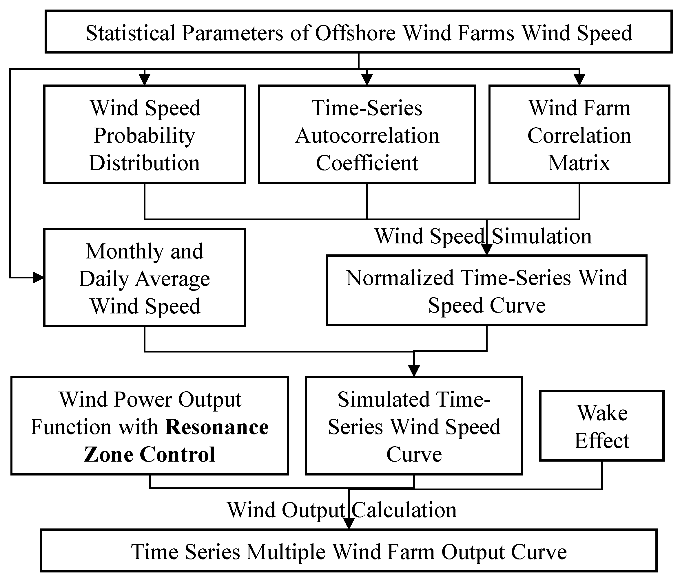
Specifically, this paper proposes an offshore wind farm simulation model considering RZ control. The framework of this model is illustrated in Figure 1.

Firstly, the time-series wind speed data of multiple offshore wind farms are utilized as the input.

Secondly, the statistical characteristics are separately calculated, including the Weibull parameters of the wind speed probability distribution, autocorrelation coefficients, the wind farm correlation matrix, and the monthly and daily average wind speed curves.

Thirdly, the SDE is applied to generate the time-series wind speed curves conforming to the statistical values. The generated raw wind speed curves are then adjusted by multiplying the per-unit monthly and daily average speed factor in accounting for the seasonal and diurnal patterns of wind speeds.

Fourthly, this paper proposes a novel wind power output function with consideration of the RZ control. By incorporating the proposed output function, the simulated wind speed curves are then adopted to generate time-series power output curves. The wind wake effect is also considered in terms of a deficiency rate.

2.2. Wind Speed Simulation Based on Stochastic Differential Equation

The stochastic differential equation introduced in [22] is applied to establish a wind speed simulation model that accounts for the spatiotemporal characteristics of wind power output. This model analytically derives the SDE for time-series wind speed considering both the autocorrelation and the Weibull shaped probability distribution function of wind speed. The SDE can be analytically derived and the time-series wind speed data are then iteratively generated by generating samples of this stochastic process at fixed time intervals.

The simulation model for a single wind farm’s operation by SDE can be briefly described as follows:

If a probability density function, $f\left(x\right)$, is non-negative, continuous, and has finite variance over its domain $\left(l,u\right)$, with its expectation, $E\left(x\right)=\mu$, then a stochastic differential equation is established:

$$d{X}_t=-\theta (X_t-\mu )dt+\sqrt{\nu \left(X_t\right)}d{W}_t,t\ge 0,$$

(1)

where $\theta \ge 0$, $W_t$ is a standard Brownian motion and $\nu \left(x\right)$ is a non-negative function.

$$\nu \left(x\right)={\displaystyle \frac{2\theta }{f\left(x\right)}}{\int }_l^x(u-y)f\left(y\right)dy,x\in (l,u)$$

(2)

Equation (1) possesses the following properties: (1) The stochastic process is ergodic, and the probability density function at each time is $f\left(x\right)$. (2) The stochastic process is mean-reverting, and its autocorrelation function satisfies the following equation.

$$\mathrm{corr}(X_{s+t},X_s)=e^{-\theta t},s,t\ge 0$$

(3)

Using the aforementioned theorem, the SDE model for wind speed is proposed. The probability distribution at each time step follows a Weibull distribution. Its autocorrelation function exhibits exponential decay. Let the wind speed follow a Weibull distribution with scale parameter c and shape parameter k:

$$f\left(x\right)={\displaystyle \frac{k}{c}}{\left({\displaystyle \frac{x}{c}}\right)}^{k-1}exp\left(-{\left({\displaystyle \frac{x}{c}}\right)}^k\right),x\ge 0$$

(4)

Then, the average wind speed, $\mu$, can be calculated as:

$$\mu =c·\Gamma \left(1+{\displaystyle \frac{1}{k}}\right),$$

(5)

where $\Gamma$ represents the Gamma function. Thus, according to the definition of $\nu \left(x\right)$ in Equation (2) and the statistic characteristics of the Weibull function, the analytical expression of $\nu \left(x\right)$ is as follows.

$$\begin{array}{cc}\hfill \nu \left(x\right)& ={\displaystyle \frac{2\theta }{f\left(x\right)}}{\int }_l^x(u-y)f\left(y\right)dy\hfill \\ \hfill & ={\displaystyle \frac{2\theta }{f\left(x\right)}}\left(\mu F\left(x\right)-{\int }_l^{x}yf\left(y\right)dy\right)\hfill \\ \hfill & ={\displaystyle \frac{2\theta c}{f\left(x\right)}}\left(\Gamma \left({\displaystyle \frac{k+1}{k}}\right)\left(1-exp\left[-{\left({\displaystyle \frac{x}{c}}\right)}^k\right]\right)-\Gamma \left({\left({\displaystyle \frac{x}{c}}\right)}^k,{\displaystyle \frac{k+1}{k}}\right)\right)\hfill \end{array}$$

(6)

In the above expression, $\Gamma \left(a\right)$ is the Gamma function and $\Gamma \left(x,a\right)$ is the incomplete Gamma function.

$$\Gamma \left(a\right)={\int }_0^{+\infty }{y}^{a-1}{e}^{-y}dy$$

(7)

$$\Gamma \left(x,a\right)={\int }_0^x{y}^{a-1}{e}^{-y}dy$$

(8)

Substituting Equation (6) into Equation (1), the value of the SDE at each time step can be computed. Therefore, the power output time series for a single wind farm, ${\widehat{v}}_t$, can be iteratively generated using the following equation:

$${\widehat{v}}_{t+1}={\widehat{v}}_t+\Delta X_t$$

(9)

Furthermore, in order to generate the time-series wind speed curves for multiple wind farms with correlated wind patterns, a multi-dimensional SDE is required. Firstly, a multi-dimensional Brownian motion, ${\mathbf{W}}_t$, where each dimension represents a standard Brownian motion, is generated. Then, the wind speed correlation matrix of the wind farms is assigned to the correlation matrix of ${\mathbf{W}}_t$. Finally, each wind farm’s time-series wind speed curve can be separately generated by applying the components of ${\mathbf{W}}_t$ to the SDE in Equation (1).

2.3. Time-Series Wind Speed Correction

The time-series wind speed curve of a wind farm is not entirely a random process but is related to climate and weather issues. The wind speed levels in the wind farm area vary across seasons and follow certain patterns. In addition, during the day, the average wind speed also fluctuates at a certain pattern due to variations in surface temperatures at different times. To account for the seasonal and diurnal patterns in wind speeds, the randomly generated wind speed curve, ${\widehat{v}}_t$, is adjusted:

$$v_t=k_h{k}_m{\widehat{v}}_t,$$

(10)

where $k_m$ represents the seasonal wind speed factor for month, m, in a year and $k_h$ represents the diurnal wind speed factor for hour, h, in a day.

Obtaining the adjusted time-series wind speed curve, $v_t$, with consideration of both the wind turbine output function and the wind farm wake effect, the wind farm’s time-series output curve can be generated by the following equation:

$$P_t=(1-\eta )C\left(k_h{k}_m{\widehat{v}}_t\right),$$

(11)

where $\eta$ is the wake effect factor. The wake effect refers to the reduction in the wind speed of the downstream turbines caused by the presence of the upstream turbines. The overall performance of the wind farm will be degraded compared to the ideal output. Therefore, $\eta$ indicates the proportion of loss of generation to the ideal output. The value of $\eta$ is usually set to 2~10%. $C\left(v\right)$ is the wind turbine output function with respect to the wind speed. In general, the function $C\left(v\right)$ follows a piece-wise shape. The power output of the turbine at wind velocities in the region between the cut-in wind speed and the rated wind speed is roughly represented by a cubic expression [7,8]. The formula of $C\left(v\right)$ is as follows:

$$C\left(v\right)=\left\{\begin{array}{cc}0,\hfill & 0\le v<v_{\mathrm{in}},v>v_{\mathrm{out}}\hfill \\ {\displaystyle \frac{v^3-v_{\mathrm{in}}^3}{v_{\mathrm{rated}}^3-v_{\mathrm{in}}^3}}R,\hfill & v_{\mathrm{in}}\le v\le v_{\mathrm{rated}}\hfill \\ R,\hfill & v_{\mathrm{rated}}\le v\le v_{\mathrm{out}}\hfill \end{array}\right.$$

(12)

where $v_{\mathrm{in}}$, $v_{\mathrm{rated}}$, and $v_{\mathrm{out}}$ are the cut-in wind speed, rated wind speed, and cut-out wind speed of the wind turbine, respectively. R is the rated wind power output.

2.4. Wind Power Output Function with Resonance Zone Control

The wind power output function, $C\left(v\right)$, in Equation (12) is an ideal one that does not consider the impact from RZ control. In this subsection, a novel wind power output function based on hysteresis control in the RZ is constructed.

The RZ control is usually implemented on the wind turbine to help the turbine speed ride through the RZ. Typically, within the RZ, if the wind speed is lower than the center of the RZ, the actual power output is set to the lower boundary of the RZ. Conversely, if the wind speed exceeds the center of the RZ, the actual power output is set to the upper boundary of the RZ.

However, when the wind speed fluctuates around the center of the RZ, frequent shifts between the upper and lower boundary outputs will occur. This leads to instability in the wind farm’s power output and causes potential mechanical damage to the wind turbine.

To address this issue, a hysteresis mechanism that takes the previous wind power output into account is then introduced. Within the RZ, a narrower buffer zone is established. If the wind speed lies within the buffer zone and the previous power output is no less than the power output at the upper boundary of the RZ, the wind power output is set to be the upper boundary. Similarly, if the wind speed lies within the buffer zone while the previous power output is no greater than the power output at the lower boundary of the RZ, the wind power output is set to be the lower boundary output.

This mechanism actively adjusts the power output when the current wind speed falls in the RZ. Therefore, the traditional power output function is supposed to be modified. The specific power output function is illustrated in Equation (13).

$$C\left(v\right)=\left\{\begin{array}{cc}0,\hfill & 0\le v<v_{\mathrm{in}},v>v_{\mathrm{out}},\hfill \\ {\displaystyle \frac{v^3-v_{\mathrm{in}}^3}{v_{\mathrm{rated}}^3-v_{\mathrm{in}}^3}}R,\hfill & v_{\mathrm{in}}\le v<v_{\mathrm{RZ},\mathrm{low}},\hfill \\ P_{\mathrm{RZ},\mathrm{low}},\hfill & v_{\mathrm{RZ},\mathrm{low}}\le v<v_{\mathrm{RZ},\mathrm{center}}-v_{\mathrm{RZ},\mathrm{buffer}},\hfill \\ P_{\mathrm{RZ},\mathrm{low}},\hfill & v_{\mathrm{RZ},\mathrm{center}}-v_{\mathrm{RZ},\mathrm{buffer}}\le v<v_{\mathrm{RZ},\mathrm{center}}+v_{\mathrm{RZ},\mathrm{buffer}},C_{\mathrm{prev}}\le P_{\mathrm{RZ},\mathrm{low}},\hfill \\ P_{\mathrm{RZ},\mathrm{high}},\hfill & v_{\mathrm{RZ},\mathrm{center}}-v_{\mathrm{RZ},\mathrm{buffer}}\le v<v_{\mathrm{RZ},\mathrm{center}}+v_{\mathrm{RZ},\mathrm{buffer}},C_{\mathrm{prev}}\ge P_{\mathrm{RZ},\mathrm{high}},\hfill \\ P_{\mathrm{RZ},\mathrm{high}},\hfill & v_{\mathrm{RZ},\mathrm{center}}+v_{\mathrm{RZ},\mathrm{buffer}}\le v<v_{\mathrm{RZ},\mathrm{high}},\hfill \\ {\displaystyle \frac{v^3-v_{\mathrm{in}}^3}{v_{\mathrm{rated}}^3-v_{\mathrm{in}}^3}}R,\hfill & v_{\mathrm{RZ},\mathrm{high}}\le v<v_{\mathrm{rated}},\hfill \\ R,\hfill & v_{\mathrm{rated}}\le v\le v_{\mathrm{out}}.\hfill \end{array}\right.$$

(13)

In Equation (13), $C_{\mathrm{prev}}$ is the wind power output at the previous time. $v_{\mathrm{RZ},\mathrm{low}},v_{\mathrm{RZ},\mathrm{center}}$, and $v_{\mathrm{RZ},\mathrm{high}}$ are the wind speeds of the lower boundary, center, and higher boundary of the RZ, respectively. $v_{\mathrm{RZ},\mathrm{buffer}}$ is the half-width of the buffer zone. $P_{\mathrm{RZ},\mathrm{high}}$ and $P_{\mathrm{RZ},\mathrm{low}}$ are the power output at the upper and lower boundaries of the RZ, respectively, which can be calculated from the original output function.

$$\begin{array}{cc}\hfill & P_{\mathrm{RZ},\mathrm{low}}={\displaystyle \frac{{v_{\mathrm{RZ},\mathrm{low}}}^3-v_{\mathrm{in}}^3}{v_{\mathrm{rated}}^3-v_{\mathrm{in}}^3}}R\hfill \end{array}$$

(14)

$$\begin{array}{cc}\hfill & P_{\mathrm{RZ},\mathrm{high}}={\displaystyle \frac{{v_{\mathrm{RZ},\mathrm{high}}}^3-v_{\mathrm{in}}^3}{v_{\mathrm{rated}}^3-v_{\mathrm{in}}^3}}R\hfill \end{array}$$

(15)

Figure 2 demonstrates the wind power output function curve that incorporates RZ control. The grey shaded area represents the RZ. The buffer zone is situated between the two dashed lines. It is clearly depicted that the wind power output exhibits a hysteresis behavior within the buffer zone. Substituting Equation (13) into Equation (10), the wind farm output simulation considering RZ control is achieved based on the simulated wind speed curves.

3. Capacity Value Assessment of Offshore Wind Farms

The concept of CV was initially utilized to evaluate the ability of thermal units, with varying forced outage rates, to provide firm capacity support (or adequacy) to the system. Due to the variation and uncertainty of offshore wind power output, wind farms cannot provide reliable power in the same way that conventional units can. This presents a significant challenge in accurately assessing the CV of offshore wind farms.

In this section, a CV assessment method based on the system’s reliability evaluation is proposed and applied to offshore wind farms. The most common metric of CV is the equivalent load-carrying capability (ELCC) [23,24]. The assessment of ELCC can be regarded as solving the equivalent reliability function, as shown in Equation (16).

$$\sum _{t\in T}{R}_t\left\{P_{w,t}+\sum _{g\in G}{C}_g,d_t+C_{cv}\right\}=\sum _{t\in T}{R}_t\left\{\sum _{g\in G}{C}_g,d_t\right\}$$

(16)

where $R_t\left(p,d\right)$ represents the reliability function of the system at time t with respect to the total available capacity, p, and the load level, d. $P_{w,t}$ is the time-series output curve of the offshore wind farm being evaluated. G is the set of conventional units in the system and $C_g$ is the installed capacity of unit g. $C_{cv}$ represents the ELCC of the evaluated offshore wind farm.

Equation (16) establishes an implicit function regarding $C_{cv}$. Solving this function yields the CV of the wind farm in the system. There are two key steps involved: (1) calculate the reliability metric, and (2) solve the implicit function.

In this paper, the expected energy not-served (EENS) is adopted as the reliability metric. With a given load or net load, $d_t$, the EENS at time interval t is calculated as shown in Equation (17).

$$R_t^{\mathrm{EENS}}\left(d_t\right)={\int }_0^{d_t}(d_t-x)P\left(x\right)\mathrm{d}\mathrm{x}$$

(17)

where $P\left(x\right)$ is the distribution of total available capacity, x, of the system’s conventional units, which can be illustrated by the capacity outage probability table (COPT) [14]. A COPT table is constructed by developing two-state or multi-state models of the conventional units and iteratively performing discrete convolution on them. This table builds the capacity levels and their associated probabilities.

The total EENS of the system during the whole evaluation period (i.e., a year) is then given by:

$$R^{\mathrm{EENS}}\left(\mathbf{d}\right)=\sum _{t=1}^T{R}_t^{\mathrm{EENS}}\left(d_t\right)$$

(18)

The COPT-based reliability function takes account of the time series information of both offshore wind power and load. It requires time-series wind power output curves. Therefore, the offshore wind farm output simulation method established in the previous section is used as a precondition for CV calculation.

The heuristic searching method is adopted to solve this implicit function of $f\left(C_{cv}\right)=0$, as indicated in Equation (16). Figure 3 demonstrates the conceptual calculation method of ELCC [25]. For the original system without the evaluated wind farm, the target EENS can be calculated by referring to the COPT table and time-series load data. Then, for the system with wind farms, by subtracting the time-series output of wind farms from the load curve, a time-series net load is obtained to calculated the EENS by Equation (18). Gradually adding the virtual loads to the net load and calculating the EENS repeatedly, the ELCC of the wind farm is determined until the target EENS is reached.

4. Case Study

The effectiveness of the proposed offshore wind power output simulation and CV evaluation model is validated using offshore wind data from Guangdong Province, China. The SDE-based offshore wind speed simulation is conducted on the chronological simulation tool GOPT software [26,27], developed by Tsinghua University. The wind power output function with RZ control is implemented in the MATLAB software (version number R2021b). The offshore wind power output and corresponding CV are also calculated in the MATLAB software.

4.1. Basic Data

Four offshore wind farms, each with a capacity of 400 MW, are selected. Based on the historical wind speed data, the statistical parameters, as shown in Figure 1, are calculated, which are then used as input parameters in the offshore wind power simulation method. The parameters of the wind turbines and the settings for the RZ are listed in

Table 1. Parameters of the wind turbines and farms.

Parameter	Value	Parameter	Value
$v_{\mathrm{in}}$	3 m/s	$v_{\mathrm{RZ},\mathrm{low}}$	5 m/s
$v_{\mathrm{rated}}$	12 m/s	$v_{\mathrm{RZ},\mathrm{high}}$	7 m/s
$v_{\mathrm{out}}$	25 m/s	$v_{\mathrm{RZ},\mathrm{buffer}}$	0.5 m/s

.

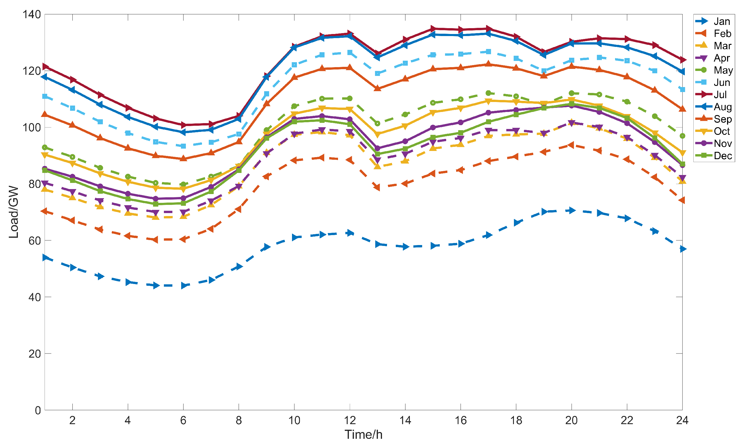
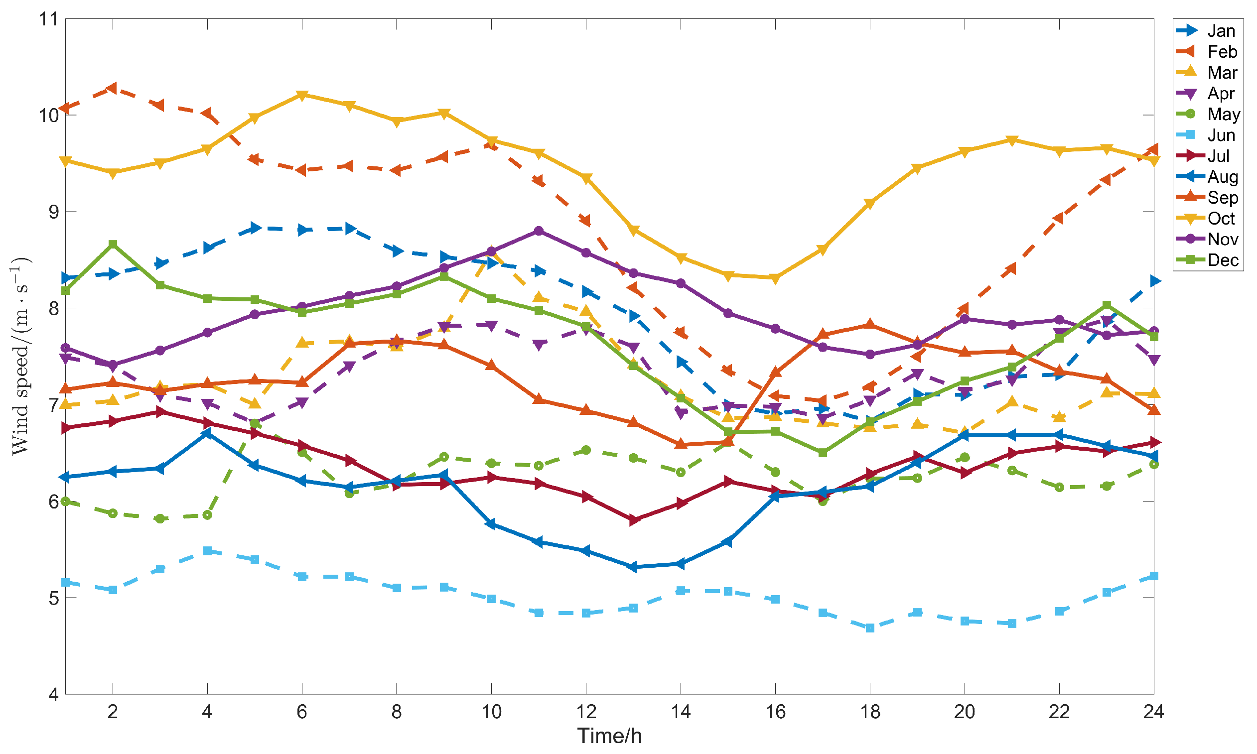
For the evaluation of the wind farms’ CV, a modified system extracted from the Guangdong grid is tested. The total installed capacity of the conventional units is nearly 150 GW, including almost 400 power units. The installed capacity of coal units is 103 GW. The total capacity of gas thermal units is 33 GW. This system also includes 10 GW from nuclear units and 3.7 GW from biomass units. The annual peak load level is set as 150 GW. Figure 4 shows the monthly average load curve. It is shown that the peak load of the system occurs in the summer, especially in July and August. From a daily perspective, the peak load usually occurs between 3 p.m. and 5 p.m. The time-series load curve will serve as the boundary condition to calculate the offshore wind farm’s CV. Moreover, Figure 5 shows the monthly average wind speed curve of a typical offshore wind farm. The overall average wind speed of this farm is more than 7 m/s. The maximum wind speed occurs in the early mornings of February and October, while in most months the wind is relatively weak in the afternoon.

4.2. Single Wind Farm Simulation

For a single offshore wind farm, its wind speed is simulated based on the proposed method. The statistical parameters of a typical wind farm are listed in

Table 2. Statistic parameters of wind speed in a typical farm.

Parameter	Value	Parameter	Value
Weibull c	8.2	Autocorrelation $\theta$	0.04
Weibull k	2.0	Wake effect $\eta$	2%

.

Figure 6 shows the probability distribution histogram of the simulated wind speed curve of a typical offshore wind farm, alongside the red line indicating the Weibull distribution function curve corresponding to the input parameters. It is noted that the probability distribution of the simulated wind speed fits well with the target Weibull distribution, which verifies the accuracy and effectiveness of the proposed method in simulating the time-series wind speed while maintaining the statistical patterns.

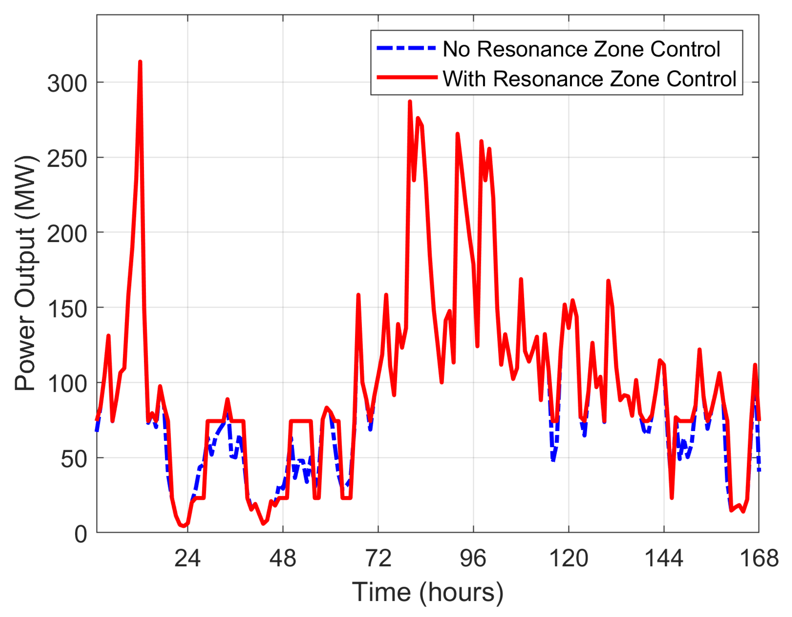
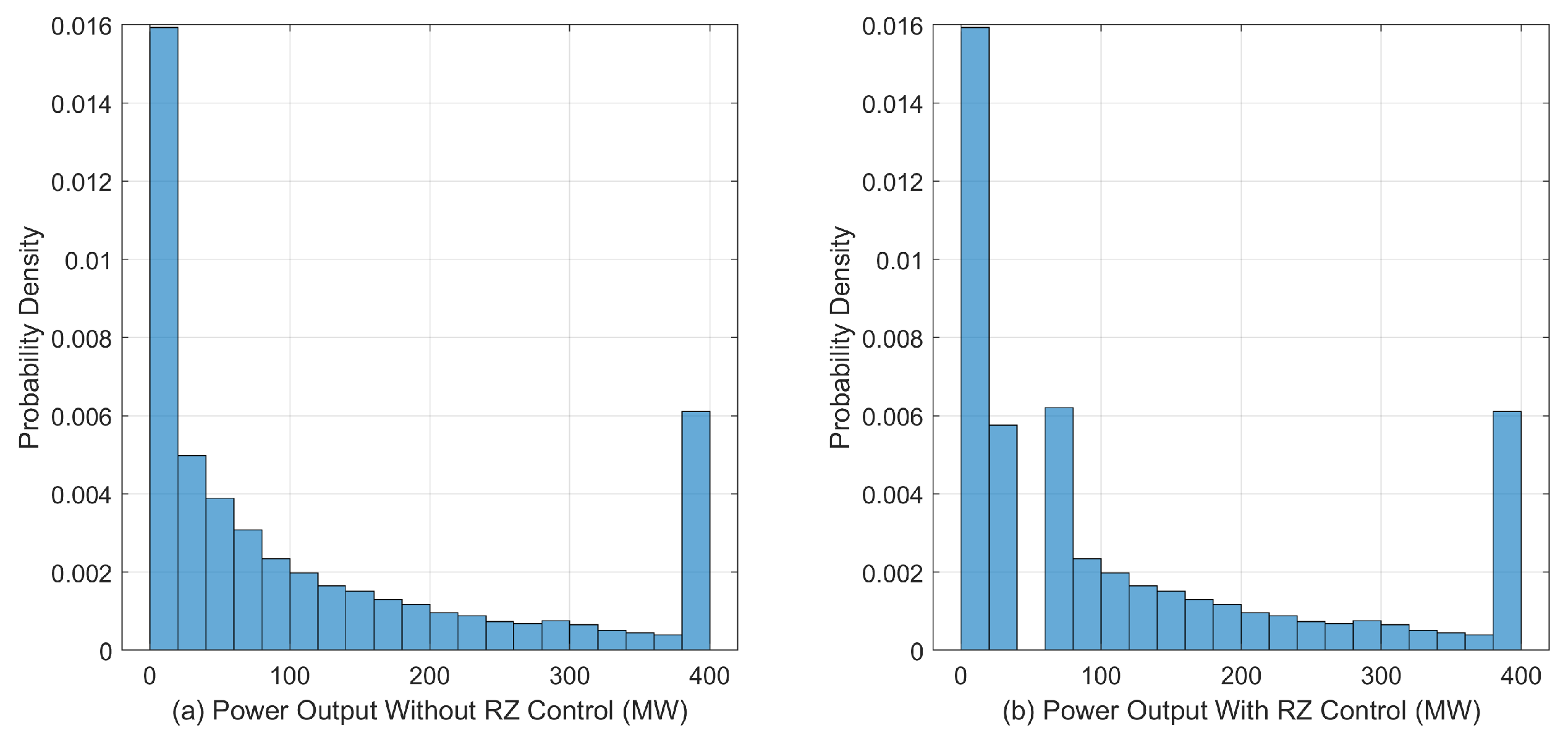
Furthermore, utilizing the power output function based on RZ control, the time-series power output curve for the offshore wind farm is established, as shown in Figure 7. Comparing with the output curve that does not consider the RZ control strategy, the wind curve from the proposed method exhibits constant performance at the upper and lower boundaries of the given RZ. Correspondingly, a probability distribution histogram of the wind power output is plotted in Figure 8, showing certain gaps at the output level of almost 10% p.u. This control strategy sharply cuts the output probability during the most severe RZ, which shows the effectiveness of the proposed wind generation simulation method with consideration of RZ control.

4.3. Multiple Wind Farm Simulation

Four offshore wind farms, which are located in Guangdong Province, China, are selected to test the output simulation and CV evaluation for multiple wind farms. Cases are selected considering different correlation scenarios for multiple wind farms and also the RZ control strategies. Then, the wind simulation and CV evaluation results for the different cases are further explored.

Four test cases are proposed, as shown in

Table 3. Case setting for multiple wind farm simulation.

Cases	Spatial Correlation	RZ Control
Case 1	Weak Correlation	No
Case 2	Weak Correlation	Yes
Case 3	Strong Correlation	No
Case 4	Strong Correlation	Yes

. On the one hand, spatial correlation is a key factor influencing the overall output of multiple wind farms. Calculated from historical wind speed data, the pairwise linear correlation coefficients between the four farms range from a maximum of 0.20 to a minimum of 0.03, which presents a weak position correlation. Moreover, a high-correlation case is established where the correlation coefficient between each two of the wind farms is set to 0.9. The correlation matrices are presented in

Table 4. Speed correlation matrix of the four wind farms under weak correlation (historical data).

	Farm 1	Farm 2	Farm 3	Farm 4
Farm 1	1.0000	0.2003	0.0410	0.1710
Farm 2	0.2003	1.0000	0.0333	0.1458
Farm 3	0.0410	0.0333	1.0000	0.0598
Farm 4	0.1710	0.1458	0.0598	1.0000

and

Table 5. Speed correlation matrix of the four wind farms under strong correlation.

	Farm 1	Farm 2	Farm 3	Farm 4
Farm 1	1.0	0.9	0.9	0.9
Farm 2	0.9	1.0	0.9	0.9
Farm 3	0.9	0.9	1.0	0.9
Farm 4	0.9	0.9	0.9	1.0

. On the other hand, in order to evaluate the impact of the RZ control strategy on the wind farms’ overall power output and CV, whether to apply the RZ control in wind power output simulation or not is another option in the case settings.

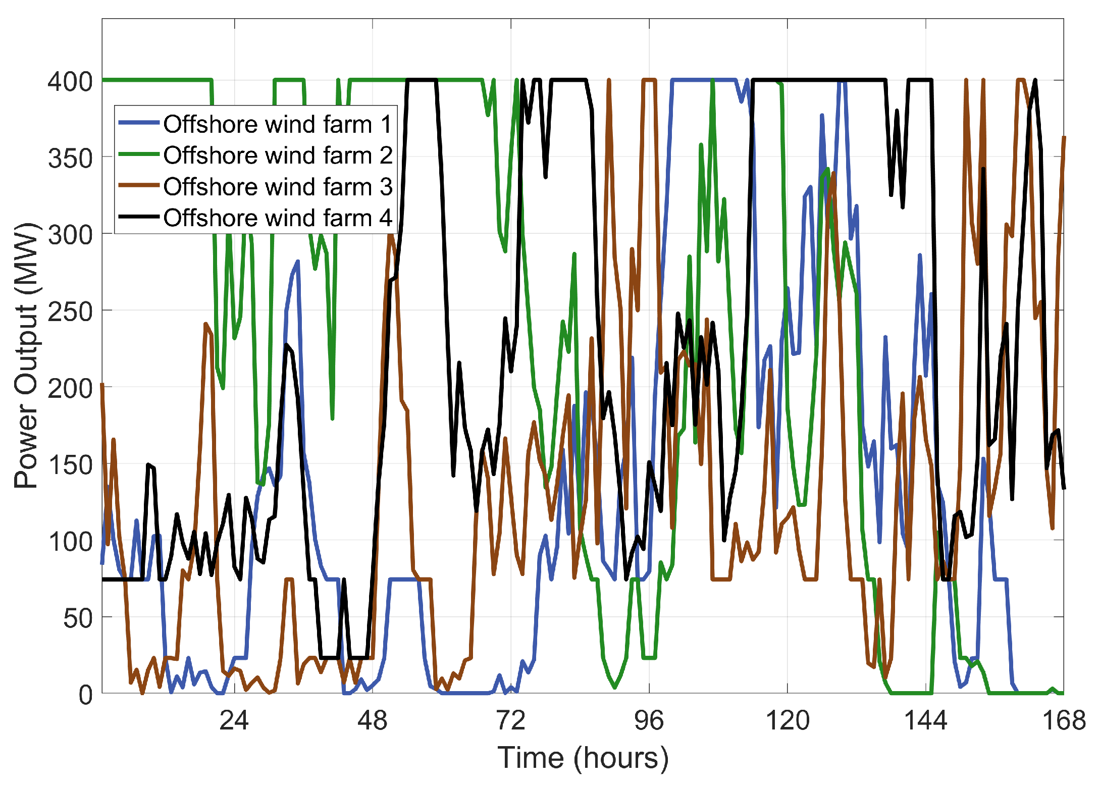
From multi-farm wind speed simulation and power generation calculation based on the output function, the time-series power output of the four offshore wind farms in a typical week are displayed in Figure 9 and Figure 10. Since the RZ control is adopted, the wind power output curves have shown the constant performance at the upper and lower boundaries of the given RZ. In Figure 9, there is rarely a correlation of the output of the offshore wind farms to each other. In the meanwhile, the output curves show some complementary patterns. Meanwhile, in Figure 10 the time-series output curves of the four farms show tight correlationship and simultaneously go up to the rated capacity or drop to zero. The simulated time-series wind power output curves corresponding to different correlation matrix inputs have proved the effectiveness of the proposed method.

Moreover, the probability distribution histograms of the combined time-series wind power output for each test case are separately presented in Figure 11.

In scenarios with weak spatial correlation (Cases 1 and 2), the total power output of four wind farms exhibits a relatively smooth probability distribution. As shown in Figure 11, the output is mainly concentrated in the lower half range (0 to 800 MW), with the highest probability occurring at around 25% of the total capacity. As the total output increases, the probability density gradually decreases. This indicates that low spatial correlation between wind farms will lead to a smoother distribution.

In contrast, for strong spatial correlation scenarios (Cases 3 and 4), the probability distribution of the total power output becomes much more diverse and fluctuant. The probability density is significantly higher in the low-output range, with the peak probability occurring at near-zero output. Additionally, there is a noticeable probability that all wind farms operate simultaneously at the rated capacity. This indicates that, with strong spatial correlation, the wind farms exhibit higher synchronicity, leading to the simultaneous occurrences of both low and high output. Consequently, the total output demonstrates greater volatility.

Comparing Case 1 with Case 2 and Case 3 with Case 4, the influence of RZ control on the probability distribution of total wind power output is relatively limited in both weak and strong correlation scenarios. In weak correlation scenarios, the smoothing effect between wind farms greatly diminishes the impact of RZ control. Meanwhile, in strong correlation scenarios, applying RZ control mainly causes that part of the output probability density at around 10% of the total capacity to be allocated into adjacent intervals. Consequently, the probability density of low power output, which is near the RZ, will become more evenly distributed.

Furthermore, based on the simulated time-series wind power output curves of the four wind farms, their total CV under different cases is calculated, as demonstrated in

Table 6. Capacity value results for the total output of the wind farms.

Cases	Capacity Value/MW	Capacity Credit
Case 1	351.58	22.0%
Case 2	353.26	22.1%
Case 3	282.62	17.7%
Case 4	285.57	17.9%

. In weak spatial correlation scenario, the CV is 351.58 MW, corresponding to 22.0% of the installed capacity, while in the strong correlation scenarios, the CV is 282.62 MW and the corresponding CC is 17.7%.

Under high correlation, the combined output shows significant low or zero output intervals. This reduces the reliable power supply capacity of the offshore wind farms, and the implementation of RZ control strategies further exacerbates this issue.

It is also noticed that, in high spatial correlation scenarios, the total output of offshore wind farms faces greater fluctuations, with a significant probability of falling into low or even zero output intervals. Therefore, the reliable generation capability of the wind farms is lower compared to weak correlation scenarios. Additionally, the impact of RZ control on the CV results appears to be marginal, since the power output range affected by the RZ control strategy is relatively small, especially when compared to the expected wind speeds of offshore farms.

4.4. Discussion

In the case study, the effectiveness of the proposed methods is verified. The impacts from both RZ control and the spatiotemporal correlation among farms on the wind power output simulation and CV evaluation are further discussed. The case results indicate that the SDE-based method can simulate the time-series wind speed while maintaining the statistical patterns of the offshore wind farm. Both the time-series wind power output curve and the output distribution indicate that RZ control will alter the wind power output distribution in low output ranges, which is in line with the boundaries of the zone. The comparison of the output results with or without RZ control shows the effectiveness of the modeling of RZ control in the wind power output function. It is also noted that weak spatial correlation of multiple farms can smooth the total output and further improve their total CV, while high correlation between farms tends to reduce the total generation reliability. For a total 1600 MW of wind farms, in weak spatial correlation scenarios the CC is 22.0%, while it is 17.7% in strong scenarios. Applying the RZ control has a marginal effect on the overall performance of multiple farms while protecting the turbines.

5. Conclusions

This paper proposes a framework for offshore wind farm output simulation with consideration of RZ control based on SDE. The SDE is adopted to simulate the uncertain wind speed while maintaining the statistic wind patterns of the farms, including the spatiotemporal correlations and wind speed distributions. Then, the RZ control is innovatively modeled in a hysteresis manner and fitted into the wind power output function. The simulated time-series speed curve is then converted to the wind power output data. Moreover, an evaluation model is proposed for the CV of offshore wind farms. The case study verifies the effectiveness of the proposed methods.

In terms of costs and economic feasibility, the proposed method can facilitate the offshore wind farms’ participation in electricity spot market bidding. Through the output simulation model for multiple farms, the operators can better predict the regional power balance situation and the market prices. Moreover, the offshore wind farm planning also relies on the long-term simulation of wind power output in a certain area. Additionally, the calculation of CV helps assess the potential for offshore wind farm participation in the capacity market.

The weaknesses of this study include the fact that the modeling of RZ control could be more detailed, particularly in considering the differences between individual turbines. Aggregating the turbines, the impact from RZ control can be better illustrated at the farm level. Furthermore, the economic issues are not discussed in the operational simulation.

Therefore, future research could explore the optimal operation and planning studies of offshore wind farms considering RZ control. With integrating both the RZ control strategies and the cost of turbine wear into long-term optimization frameworks, future studies will help offshore wind farm investors and system operators make better decision. Furthermore, the harmonic stability and power quality issues that come from the wind power output control should be considered in future offshore wind operation studies.

References

Global Wind Energy Council. Global Offshore Wind Report 2024; Global Wind Energy Council: Brussels, Belgium, 2024. [Google Scholar]
Yeh, T.-H.; Wang, L. A Study on Generator Capacity for Wind Turbines Under Various Tower Heights and Rated Wind Speeds Using Weibull Distribution. IEEE Trans. Energy Convers.2008, 23, 592–602. [Google Scholar] [CrossRef]
Sweetman, B.; Dai, S. Transformation of Wind Turbine Power Curves Using the Statistics of the Wind Process. IEEE Trans. Sustain. Energy2021, 12, 2053–2061. [Google Scholar] [CrossRef]
Zhang, N.; Kang, C.; Duan, C.; Tang, X.; Huang, J.; Lu, Z.; Wang, W.; Qi, J. Simulation Methodology of Multiple Wind Farms Operation Considering Wind Speed Correlation. Int. J. Power Energy Syst.2010, 30, 264–273. [Google Scholar] [CrossRef]
Abdelaziz, S.; Sparrow, S.N.; Hua, W.; Wallom, D. Extreme Wind Gust Impact on UK Offshore Wind Turbines: Long-Term Return Level Estimation. In Proceedings of the 2023 IEEE Power & Energy Society General Meeting (PESGM), Orlando, FL, USA, 16–20 July 2023; pp. 1–5. [Google Scholar]
Liu, Y.; Li, S.; Chan, P.W.; Chen, D. Empirical Correction Ratio and Scale Factor to Project the Extreme Wind Speed Profile for Offshore Wind Energy Exploitation. IEEE Trans. Power Syst.2017, 32, 872–881. [Google Scholar] [CrossRef]
Mathew, S. Performance of wind energy conversion systems. In Wind Energy: Fundamentals, Resource Analysis and Economics; Springer: Berlin/Heidelberg, Germany, 2006; pp. 145–178. ISBN 978-3-540-30906-2. [Google Scholar] [CrossRef]
Carrillo, C.; Obando Montaño, A.F.; Cidrás, J.; Díaz-Dorado, E. Review of power curve modelling for wind turbines. Renew. Sustain. Energy Rev.2013, 21, 572–581. [Google Scholar] [CrossRef]
Philippe, W.P.J.; Eftekharnejad, S.; Ghosh, P.K. A Copula-Based Uncertainty Modeling of Wind Power Generation for Probabilistic Power Flow Study. In Proceedings of the 2019 IEEE 7th International Conference on Smart Energy Grid Engineering (SEGE), Oshawa, ON, Canada, 12–14 August 2019; pp. 218–222. [Google Scholar]
Feijóo, A.; Villanueva, D. Four-Parameter Models for Wind Farm Power Curves and Power Probability Density Functions. IEEE Trans. Sustain. Energy2017, 8, 1783–1784. [Google Scholar] [CrossRef]
Wu, Y.K.; Su, P.E.; Su, Y.S.; Wu, T.Y. Economics- and reliability-based design for an offshore wind farm. IEEE Trans. Power Syst.2017, 32, 1743–1752. [Google Scholar] [CrossRef]
Acaroğlu, H.; García Márquez, F.P. High voltage direct current systems through submarine cables for offshore wind farms: A life-cycle cost analysis with voltage source converters for bulk power transmission. Energy2022, 247, 123310. [Google Scholar] [CrossRef]
Acaroğlu, H.; García Márquez, F.P. Comprehensive Review on Electricity Market Price and Load Forecasting Based on Wind Energy. Energies2021, 14, 7473. [Google Scholar] [CrossRef]
Keane, A.; Milligan, M.; Dent, C.J.; Hasche, B.; D’Annunzio, C.; Dragoon, K.; Holttinen, H.; Samaan, N.; Söder, L.; O’Malley, M. Capacity Value of Wind Power. IEEE Trans. Power Syst.2011, 26, 564–572. [Google Scholar] [CrossRef]
Zhang, N.; Yu, Y.; Fang, C.; Su, Y.; Kang, C. Power System Adequacy with Variable Resources: A Capacity Credit Perspective. IEEE Trans. Reliab.2024, 73, 53–58. [Google Scholar] [CrossRef]
Zhang, N.; Kang, C.; Kirschen, D.S.; Xia, Q. Rigorous Model for Evaluating Wind Power Capacity Credit. IET Renew. Power Gener.2013, 7, 504–513. [Google Scholar] [CrossRef]
Frew, B.; Cole, W.; Sun, Y.; Richards, J.; Mai, T. 8760-Based Method for Representing Variable Generation Capacity Value in Capacity Expansion Models; NREL/CP-6A20-68869; NREL: Golden, CO, USA, 2017. [Google Scholar]
Zuo, H.; Bi, K.; Hao, H. A State-of-the-Art Review on the Vibration Mitigation of Wind Turbines. Renew. Sustain. Energy Rev.2020, 121, 109710. [Google Scholar] [CrossRef]
Li, Z.; Tian, S.; Zhang, Y.; Li, H.; Lu, M. Active Control of Drive Chain Torsional Vibration for DFIG-Based Wind Turbine. Energies2019, 12, 1744. [Google Scholar] [CrossRef]
Licari, J.; Ekanayake, J.B.; Jenkins, N. Investigation of a Speed Exclusion Zone to Prevent Tower Resonance in Variable-Speed Wind Turbines. IEEE Trans. Sustain. Energy2013, 4, 977–984. [Google Scholar] [CrossRef]
Wang, J.; Golnary, F.; Li, S.; Weerasuriya, A.U.; Tse, K.T. A Review on Power Control of Wind Turbines with the Perspective of Dynamic Load Mitigation. Ocean Eng.2024, 311, 118806. [Google Scholar] [CrossRef]
Bibby, B.M.; Skovgaard, I.M.; Sørensen, M. Diffusion-Type Models with Given Marginal Distribution and Autocorrelation Function. Bernoulli2005, 11, 191–220. [Google Scholar] [CrossRef]
Milligan, M.; Frew, B.; Ibanez, E.; Kiviluoma, J.; Holttinen, H.; Söder, L. Capacity Value Assessments of Wind Power. WIREs Energy Environ.2017, 6, e226. [Google Scholar] [CrossRef]
Milligan, M.; Porter, K. The Capacity Value of Wind in the United States: Methods and Implementation. Electr. J.2006, 19, 91–99. [Google Scholar] [CrossRef]
Zhou, Y.; Mancarella, P.; Mutale, J. Framework for Capacity Credit Assessment of Electrical Energy Storage and Demand Response. IET Gener. Transm. Distrib.2016, 10, 2267–2276. [Google Scholar] [CrossRef]
Zhang, N.; Kang, C.; Xia, Q.; Ding, Y.; Huang, Y.; Sun, R.; Huang, J.; Bai, J. A Convex Model of Risk-Based Unit Commitment for Day-Ahead Market Clearing Considering Wind Power Uncertainty. IEEE Trans. Sustain. Energy2015, 30, 1582–1592. [Google Scholar] [CrossRef]
Figure 1.
Flowchart of the wind farm simulation framework.
Figure 2.
Wind turbine output characteristic curve under RZ Control.
Figure 3.
Conceptual calculation method of ELCC.
Figure 4.
Load profile: monthly average load curve.
Figure 5.
Wind profile: monthly average wind speed curve.
Figure 6.
Probability density of simulated wind speed vs. Weibull distribution.
Figure 7.
Wind power curve in a typical week with/without RZ control.
Figure 8.
Probability density of the single farm’s output w.o. (a)/with (b) RZ control.
Figure 9.
Wind power curves in a typical week for four offshore wind farms under weak correlation.
Figure 10.
Wind power curves in a typical week for four offshore wind farms under strong correlation.
Figure 11.
Probability density of the total simulated output of the four offshore wind farms under different cases: (a) Cases 1 and 2. (b) Cases 3 and 4.