
Mini-Review on the Design Principles of Biochemical Oscillators for the Continuous Ethanol Fermentation Processes


Abstract
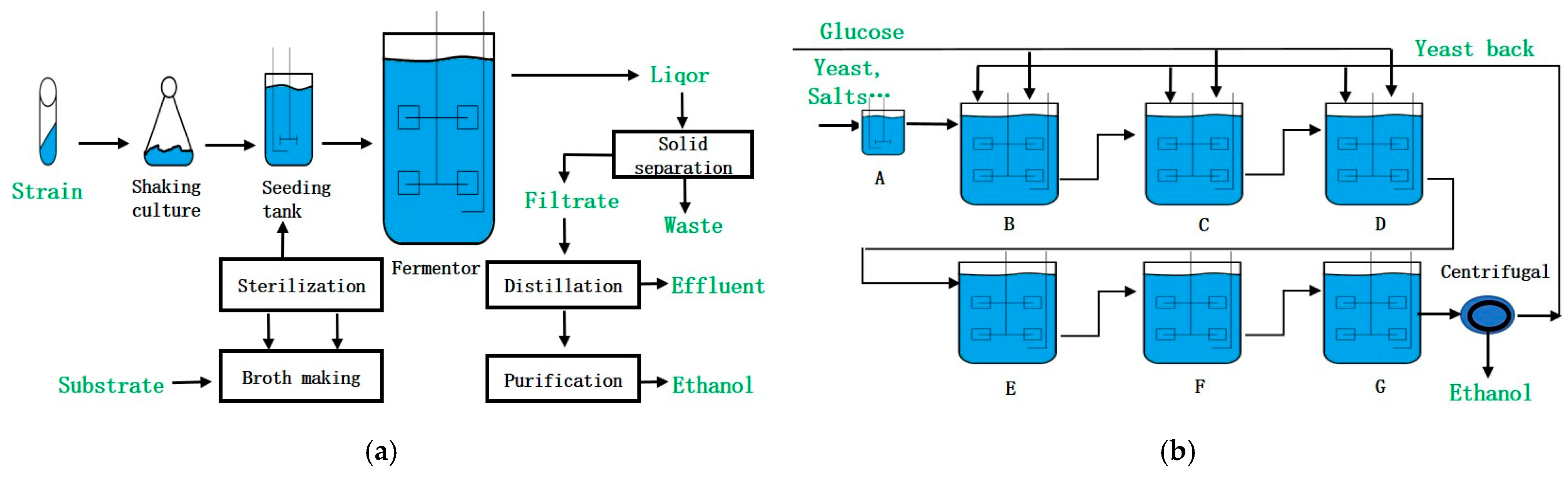
1. Introduction
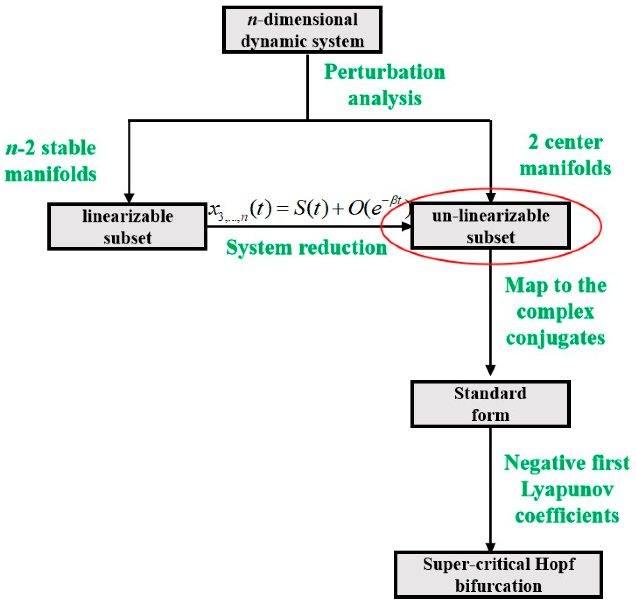
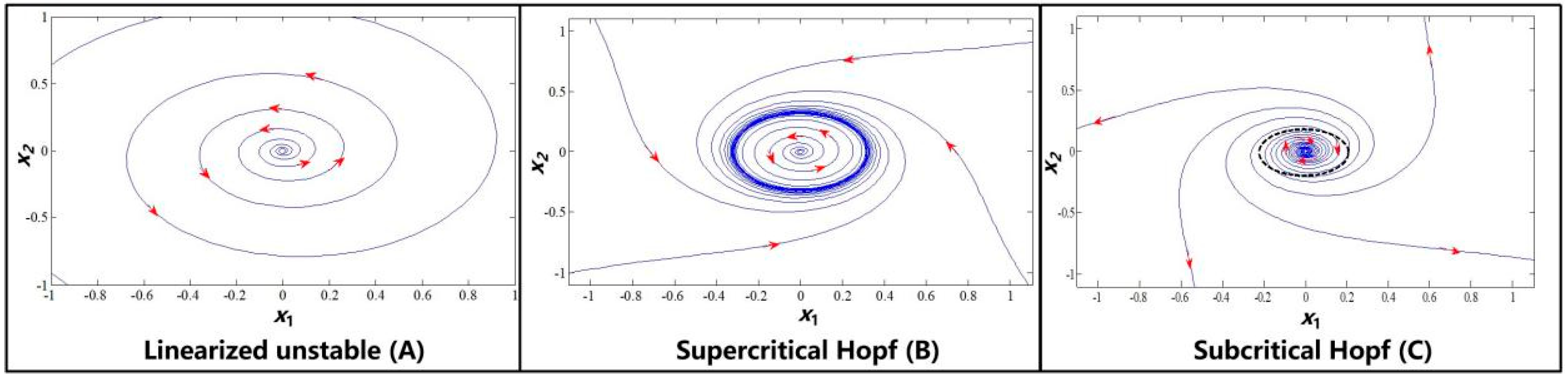
2. Preliminaries of the Hopf Bifurcation and Limit Cycles
3. Mechanisms of the Biochemical Oscillators
3.1. Negative Feedback
3.2. Nonlinear Feedback
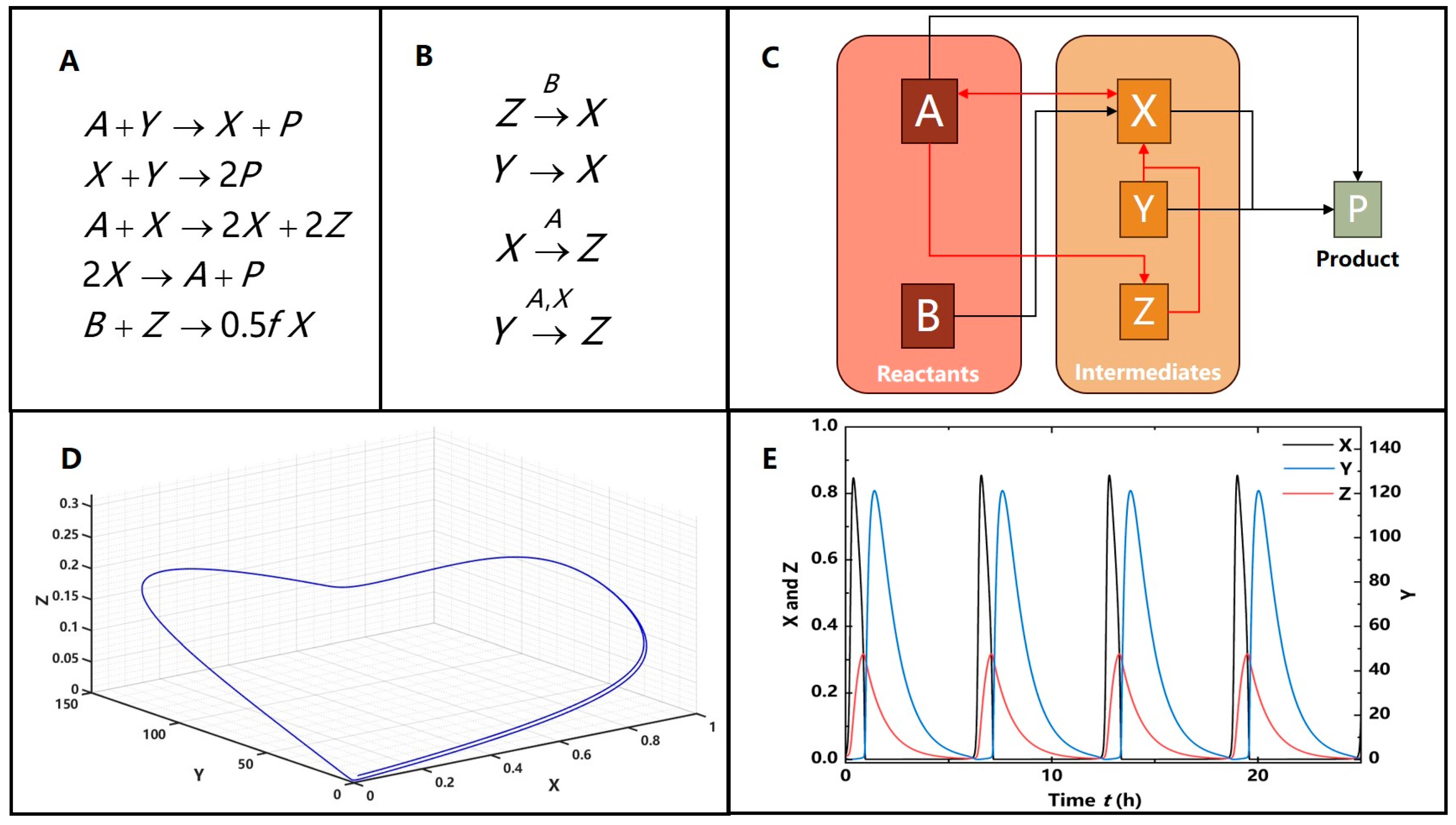
3.2.1. The Illustrative Example of Nonlinear Feedback
3.2.2. Nonlinearity Induced Limit Cycles in the Feedback


3.3. Auto-Catalytic/Positive-Plus Feedback
3.3.1. The Illustrative Example of Positive-Plus Feedback
3.3.2. Auto-Catalytic Elements in the Feedback
3.4. Delay Feedback
3.4.1. The Illustrative Example of Delay Feedback
3.4.2. Time Delay in the Feedback
4. Conclusions
Author Contributions
Funding
Data Availability Statement
Conflicts of Interest
Nomenclature
| D | dilution rate (h−1) |
| F | flow rate (l/h) |
| Ki | ethanol inhibition coefficient (g/L) |
| ks | the half-saturation constant (g/L) |
| n | fermentation cycle |
| P | product concentration (g/L) |
| r | the part of broth discharged and refilled (%) |
| S | substrate concentration (g/L) |
| Sin | the limiting substrate input concentration (g/L) |
| V | the constant volume of the tank (L) |
| X | biomass concentration (g/L) |
| Yxp | substrate consumption ratio for per product (g/g) |
| Yxs | substrate consumption ratio for per biomass produced (g/g) |
| γ | the break-even value of substrate (g/L) |
| ε | the time taken to empty and refill the tank (h) |
| μ | the characteristic reaction rates of biomass concentration (h−1) |
| μm | the maximum growth rate (h−1) |
| ρ | the characteristic reaction rates of product concentration (h−1) |
| σ | the characteristic reaction rates of substrate concentration (h−1) |
| τ | the period of evaluation |
References
- Melendez, J.R.; Matyas, B.; Hena, S.; Lowy, D.A.; El Salous, A. Perspectives in the production of bioethanol: A review of sustainable methods, technologies, and bioprocesses. Renew. Sustain. Energy Rev. 2022, 160, 112260. [Google Scholar] [CrossRef]
- Baeyens, J.; Kang, Q.; Appels, L.; Dewil, R.; Lv, Y.; Tan, T. Challenges and opportunities in improving the production of bio-ethanol. Prog. Energy Combust. Sci. 2015, 47, 60–88. [Google Scholar] [CrossRef]
- Akhtar, N.; Gupta, K.; Goyal, D.; Goyal, A. Recent advances in pretreatment technologies for efficient hydrolysis of lignocellulosic biomass. Environ. Prog. Sustain. Energy 2016, 35, 489–511. [Google Scholar] [CrossRef]
- Sun, C.; Meng, X.; Sun, F.; Zhang, J.; Tu, M.; Chang, J.S.; Reungsang, A.; Xia, A.; Ragauskas, A.J. Advances and perspectives on mass transfer and enzymatic hydrolysis in the enzyme-mediated lignocellulosic biorefinery: A review. Biotechnol. Adv. 2023, 62, 108059. [Google Scholar] [CrossRef]
- Brunecky, R.; Donohoe, B.S.; Yarbrough, J.M.; Mittal, A.; Scott, B.R.; Ding, H.; Taylor II, L.E.; Russell, J.F.; Chung, D.; Westpheling, J.; et al. The multi domain Caldi cellulosiruptor bescii CelA cellulase excels at the hydrolysis of crystalline cellulose. Sci. Rep. 2017, 7, 9622. [Google Scholar] [CrossRef]
- Nguyen, T.Y.; Cai, C.M.; Kumar, R.; Wyman, C.E. Overcoming factors limiting high-solids fermentation of lignocellulosic biomass to ethanol. Proc. Natl. Acad. Sci. USA 2017, 114, 11673–11678. [Google Scholar] [CrossRef]
- Fan, S.; Xiao, Z.; Zhang, Y.; Tang, X.; Chen, C.; Li, W.; Deng, Q.; Yao, P. Enhanced ethanol fermentation in a pervaporation membrane bioreactor with the convenient permeate vapor recovery. Bioresour. Technol. 2014, 155, 229–234. [Google Scholar] [CrossRef]
- Wang, J.; Chae, M.; Sauvageau, D.; Bressler, D.C. Improving ethanol productivity through self-cycling fermentation of yeast: A proof of concept. Biotechnol. Biofuels 2017, 10, 1–11. [Google Scholar] [CrossRef]
- dos Santos, L.; de Barros Grassi, M.C.; Gallardo, J.C.M.; Pirolla, R.; Calderón, L.L.; De Carvalho-Netto, O.V.; Parreiras, L.; Camargo, E.L.O.; Drezza, A.L.; Missawa, S.K.; et al. Second-generation ethanol: The need is becoming a reality. Ind. Biotechnol. 2016, 12, 40–57. [Google Scholar] [CrossRef]
- Takahashi, C.N.; Miller, A.W.; Ekness, F.; Dunham, M.J.; Klavins, E. A low cost, customizable turbidostat for use in synthetic circuit characterization. ACS Synth. Biol. 2015, 4, 32–38. [Google Scholar] [CrossRef]
- Müller, I. A History of Thermodynamics: The Doctrine of Energy and Entropy; Springer Science & Business Media: Berlin/Heidelberg, Germany, 2007. [Google Scholar]
- Meissner, W. Max Planck, the man and his work. Science 1951, 113, 75–81. [Google Scholar] [CrossRef] [PubMed]
- Bertola, V.; Cafaro, E. A critical analysis of the minimum entropy production theorem and its application to heat and fluid flow. Int. J. Heat Mass Transf. 2008, 51, 1907–1912. [Google Scholar] [CrossRef]
- Prigogine, I. Time, Structure, and Fluctuation. Science 1978, 201, 777–785. [Google Scholar] [CrossRef] [PubMed]
- Lee, K.J.; Tribe, D.E.; Rogers, P.L. Ethanol production by Zymomonas mobilis in continuous culture at high glucose concentrations. Biotechnol. Lett. 1979, 1, 421–426. [Google Scholar]
- Ghommidh, C.; Vaija, J.; Bolarinwa, S.; Navarro, J.M. Oscillatory behaviour of Zymomonas in continuous cultures: A simple stochastic model. Biotechnol. Lett. 1989, 11, 659–664. [Google Scholar] [CrossRef]
- Borzani, W. Variation of the ethanol yield during oscillatory concentrations changes in undisturbed continuous ethanol fermentation of sugar-cane blackstrap molasses. World J. Microbiol. Biotechnol. 2001, 17, 253–258. [Google Scholar] [CrossRef]
- Chen, L.J.; Xu, Y.L.; Bai, F.W.; Anderson, W.A.; Moo-Young, M. Observed quasi-steady kinetics of yeast cell growth and ethanol formation under very high gravity fermentation condition. Biotechnol. Bioprocess Eng. 2005, 10, 115–121. [Google Scholar] [CrossRef]
- Ge, X.M.; Zhao, X.Q.; Bai, F.W. Online monitoring and characterization of flocculating yeast cell flocs during continuous ethanol fermentation. Biotechnol. Bioeng. 2005, 90, 523–531. [Google Scholar] [CrossRef]
- Bai, F.W.; Chen, L.J.; Anderson, W.A.; Moo-Young, M. Parameter oscillations in very high gravity medium continuous ethanol fermentation and their attenuation on multi-stage packed column bioreactor system. Biotechnol. Bioeng. 2004, 88, 558–566. [Google Scholar] [CrossRef]
- Dano, S.; Sørensen, P.G.; Hynne, F. Sustained oscillations in living cells. Nature 1999, 402, 320–322. [Google Scholar] [CrossRef]
- Wolf, J.; Heinrich, R. Effect of cellular interaction on glycolytic oscillations in yeast: A theoretical investigation. Biochem. J. 2000, 345, 321–334. [Google Scholar] [CrossRef] [PubMed]
- Ferrell, J.E., Jr. Feedback loops and reciprocal regulation: Recurring motifs in the systems biology of the cell cycle. Curr. Opin. Cell Biol. 2013, 25, 676–686. [Google Scholar] [CrossRef] [PubMed]
- Tyson, J.J.; Novak, B. Regulation of the eukaryotic cell cycle: Molecular antagonism, hysteresis, and irreversible transitions. J. Theor. Biol. 2001, 210, 249–263. [Google Scholar] [CrossRef] [PubMed]
- Harashima, H.; Dissmeyer, N.; Schnittger, A. Cell cycle control across the eukaryotic kingdom. Trends Cell Biol. 2013, 23, 345–356. [Google Scholar] [CrossRef]
- Sunchu, B.; Cabernard, C. Principles and mechanisms of asymmetric cell division. Development 2020, 147, dev167650. [Google Scholar] [CrossRef]
- Crosby, M.E. Cell cycle: Principles of control. Yale J. Biol. Med. 2007, 80, 141. [Google Scholar]
- Barnum, K.J.; O’Connell, M.J. Cell cycle regulation by checkpoints. In Cell Cycle Control: Mechanisms and Protocols; Humana Press: New York, NY, USA, 2014; pp. 29–40. [Google Scholar]
- Alon, U. Network motifs: Theory and experimental approaches. Nat. Rev. Genet. 2007, 8, 450–461. [Google Scholar] [CrossRef]
- Tyson, J.J.; Novak, B. Functional motifs in biochemical reaction networks. Annu. Rev. Phys. Chem. 2010, 61, 219–240. [Google Scholar] [CrossRef]
- Hobley, T.J.; Pamment, N.B. Differences in response of Zymomonasmobilis and Saccharomyces cerevisiae to change in extracellular ethanol concentration. Biotechnol. Bioeng. 1994, 43, 155–158. [Google Scholar] [CrossRef]
- Li, C.C. Mathematical models of ethanol inhibition effects during alcohol fermentation. Nonlinear Anal. Theory Methods Appl. 2009, 71, e1608–e1619. [Google Scholar] [CrossRef]
- Jöbses, I.M.L.; Egberts, G.T.C.; Luyben, K.C.A.M.; Roels, J.A. Fermentation kinetics of Zymomonasmobilis at high ethanol concentrations: Oscillations in continuous cultures. Biotechnol. Bioeng. 1986, 28, 868–877. [Google Scholar] [CrossRef] [PubMed]
- Xiu, Z.L.; Zeng, A.P.; Deckwer, W.D. Multiplicity and stability analysis of microorganisms in continuous culture: Effects of metabolic overflow and growth inhibition. Biotechnol. Bioeng. 1998, 57, 251–261. [Google Scholar] [CrossRef]
- Ma, Y.F.; Xiu, Z.L.; Sun, L.H.; Feng, E.M. Hopf bifurcation and chaos analysis of a microbial continuous culture model with time delay. Int. J. Nonlinear Sci. Numer. Simul. 2006, 7, 305–308. [Google Scholar] [CrossRef]
- Lian, H.; Feng, E.; Li, X.; Ye, J.; Xiu, Z. Oscillatory behavior in microbial continuous culture with discrete time delay. Nonlinear Anal. Real World Appl. 2009, 10, 2749–2757. [Google Scholar] [CrossRef]
- Skupin, P.; Metzger, M. Stability analysis of the continuous ethanol fermentation process with a delayed product inhibition. Appl. Math. Model. 2017, 49, 48–58. [Google Scholar] [CrossRef]
- Caicedo-Casso, A.; Kang, H.W.; Lim, S.; Hong, C.I. Robustness and period sensitivity analysis of minimal models for biochemical oscillators. Sci. Rep. 2015, 5, 13161. [Google Scholar] [CrossRef]
- Jiménez, A.; Lu, Y.; Jambhekar, A.; Lahav, G. Principles, mechanisms and functions of entrainment in biological oscillators. Interface Focus 2022, 12, 20210088. [Google Scholar] [CrossRef]
- Robinett III, R.D.; Wilson, D.G. What is a limit cycle? Int. J. Control 2008, 81, 1886–1900. [Google Scholar] [CrossRef]
- Rosenfeld, N.; Elowitz, M.B.; Alon, U. Negative autoregulation speeds the response times of transcription networks. J. Mol. Biol. 2002, 323, 785–793. [Google Scholar] [CrossRef]
- Becskei, A.; Serrano, L. Engineering stability in gene networks by autoregulation. Nature 2000, 405, 590–593. [Google Scholar] [CrossRef]
- Novak, B.; Tyson, J.J. Design principles of biochemical oscillators. Nat. Rev. Mol. Cell. Biol. 2008, 9, 981–991. [Google Scholar] [CrossRef] [PubMed]
- Ferrell, J.E., Jr.; Tsai, T.Y.; Yang, Q. Modeling the cell cycle: Why do certain circuits oscillate? Cell 2011, 144, 874–885. [Google Scholar] [CrossRef] [PubMed]
- Thomas, R. On the relation between the logical structure of systems and their ability to generate multiple steady states or sustained oscillations. In Numerical Methods in the Study of Critical Phenomena; Springer Series in Synergetics; Springer: Berlin/Heidelberg, Germany, 1981; Volume 9, pp. 180–193. [Google Scholar]
- Richard, A.; Comet, J.P. Stable periodicity and negative circuits in differential systems. J. Math. Biol. 2011, 63, 593–600. [Google Scholar] [CrossRef] [PubMed]
- Larue, F.; Lafon-Lafourcade, S.; Ribereau-Gayon, P. Relationship between the inhibition of alcoholic fermentation by Saccharomyces cerevisiae and the activities of hexokinase and alcohol dehydrogenase. Biotechnol. Lett. 1984, 6, 687–692. [Google Scholar] [CrossRef]
- Casey, G.P.; Ingledew, W.M. Ethanol tolerance in yeasts. Crit. Rev. Microbiol. 1986, 13, 219–280. [Google Scholar] [CrossRef]
- Jones, A.M.; Ingledew, W.M. Fuel alcohol production: Optimizing of temperature for efficient very-high-gravity fermentation. Appl. Environ. Microbiol. 1994, 60, 1048–1051. [Google Scholar] [CrossRef]
- You, K.M.; Rosenfield, C.L.; Knipple, D.C. Ethanol tolerance in the yeast Saccharomyces cerevisiae is dependent on cellular oleic acid content. Appl. Environ. Microbiol. 2003, 69, 1499–1503. [Google Scholar] [CrossRef]
- Ryu, D.D.Y.; Kim, Y.J.; Kim, J.H. Effect of air supplement on the performance of continuous ethanol fermentation system. Biotechnol. Bioeng. 1984, 26, 12–16. [Google Scholar] [CrossRef]
- Pascual, C.; Alonso, A.; Garcia, I.; Roman, C.; Kotyk, A. Effect of ethanol on glucose transport, key glycolytic enzymes, and proton extrusion in Saccharomyces cerevisiae. Biotechnol. Bioeng. 1986, 32, 374–378. [Google Scholar] [CrossRef]
- Salguerio, S.P.; Sa-Correia, I.; Novais, J.M. Ethanol induced-leakage in Saccharomyces cerevisiae: Kinetics and relationship to yeast ethanol tolerance and alcohol fermentation productivity. Appl. Environ. Microbiol. 1988, 54, 903–909. [Google Scholar] [CrossRef]
- Cartwright, C.P.; Veazey, F.J.; Rose, A.H. Effect of ethanol on activity of the plasma-membrane ATPase in and accumulation of glycine by Saccharomyces cerevisiae. J. Gen. Microbiol. 1987, 133, 857–865. [Google Scholar] [CrossRef] [PubMed]
- Rosa, M.F.; Sa-Correia, I. Ethanol tolerance and activity of plasma membrane ATPase in Kluyveromyces marxianus and Saccharomyces cerevisiae. Enzym. Microb. Technol. 1992, 14, 23–27. [Google Scholar] [CrossRef]
- Yang, Q.; Ferrell, J.E., Jr. The Cdk1–APC/C cell cycle oscillator circuit functions as a time-delayed, ultrasensitive switch. Nat. Cell Biol. 2013, 15, 519–525. [Google Scholar] [CrossRef] [PubMed]
- Zhou, S.; Zhang, W.; Zhang, Y.; Ni, X.; Li, Z. Bifurcation and oscillatory dynamics of delayed CDK1-APC feedback loop. IET Syst. Biol. 2020, 14, 297–306. [Google Scholar] [CrossRef] [PubMed]
- Orlando, D.A.; Lin, C.Y.; Bernard, A.; Wang, J.Y.; Socolar, J.E.; Iversen, E.S.; Hartemink, A.J.; Haase, S.B. Global control of cell-cycle transcription by coupled CDK and network oscillators. Nature 2008, 453, 944–947. [Google Scholar] [CrossRef]
- Simmons Kovacs, L.A.; Mayhew, M.B.; Orlando, D.A.; Jin, Y.; Li, Q.; Huang, C.; Reed, S.I.; Mukherjee, S.; Haase, S.B. Cyclin-dependent kinases are regulators and effectors of oscillations driven by a transcription factor network. Mol. Cell 2012, 45, 669–679. [Google Scholar] [CrossRef]
- Zhai, C.; Sun, W. Analytical approximation of a self-oscillatory reaction system using the Laplace-Borel transform. Chaos Solitons Fractals 2021, 142, 110508. [Google Scholar] [CrossRef]
- Chi, Z. Analytical and numerical computation of self-oscillating gels driven by the Belousov-Zhabotinsky reaction. Phys. Scr. 2024, 99, 025229. [Google Scholar] [CrossRef]
- Lotka, A.J. Undamped oscillations derived from the law of mass action. J. Am. Chem. Soc. 1920, 42, 1595–1599. [Google Scholar] [CrossRef]
- Richard, P. The rhythm of yeast. FEMS Microbiol. Rev. 2003, 27, 547–557. [Google Scholar] [CrossRef]
- Ghosh, A.; Chance, B. Oscillations of glycolytic intermediates in yeast cells. Biochem. Biophys. Res. Commun. 1964, 16, 174–181. [Google Scholar] [CrossRef] [PubMed]
- Tu, B.P.; Kudlicki, A.; Rowicka, M.; McKnight, S.L. Logic of the yeast metabolic cycle: Temporal compartmentalization of cellular processes. Science 2005, 310, 1152–1158. [Google Scholar] [CrossRef] [PubMed]
- Satroutdinov, A.D.; Kuriyama, H.; Kobayashi, H. Oscillatory metabolism of Saccharomyces cerevisiae in continuous culture. FEMS Microbiol. Lett. 1992, 77, 261–267. [Google Scholar] [CrossRef] [PubMed]
- Palkova, Z.; Devaux, F.; Icicova, M.; Minarikova, L.; Le Crom, S.; Jacq, C. Ammonia pulses and metabolic oscillations guide yeast colony development. Mol. Biol. Cell 2002, 13, 3901–3914. [Google Scholar] [CrossRef]
- Higgins, J. The theory of oscillating reactions. Ind. Eng. Chem. 1967, 59, 18–62. [Google Scholar] [CrossRef]
- Richter, O.; Betz, A.; Giersch, C. The response of oscillating glycolysis to perturbations in the NADH/NAD system: A comparison between experiments and a computer model. BioSystems 1975, 7, 137–146. [Google Scholar] [CrossRef]
- Selkov, E.E. Stabilisation of energy charge, generation of oscillation and multiple steady states in energy metabolism as a result of purely stoichiometric regulation. Eur. J. Biochem. 1975, 59, 151–157. [Google Scholar] [CrossRef]
- Bier, M.; Bakker, B.M.; Westerho, H.V. How yeast cells synchronize their glycolytic oscillations: A perturbation analytic treatment. Biophys. J. 2000, 78, 1087–1093. [Google Scholar] [CrossRef]
- Wolf, J.; Sohn, H.; Heinrich, R.; Kuriyama, H. Mathematical analysis of a mechanism for autonomous metabolic oscillations in continuous culture of Saccharomyces cerevisiae. FEBS Lett. 2001, 499, 230–234. [Google Scholar] [CrossRef]
- Prigogine, I. From Being to Becoming, Time and Complexity in Physical Sciences; Freeman: San Francisco, CA, USA, 1979. [Google Scholar]
- Crooker, P.S.; Wei, C.; Tanner, R.D. The effect of the specific growth rate and yield expressions on the existence of oscillatory behavior of a continuous fermentation model. Chem. Eng. Commun. 1980, 6, 333–347. [Google Scholar] [CrossRef]
- Thatipamala, R.; Rohani, S.; Hill, G.A. Effects of high product and substrate inhibitions on the kinetics and biomass and product yields during ethanol batch fermentation. Biotechnol. Bioeng. 1992, 40, 289–297. [Google Scholar] [CrossRef] [PubMed]
- Groot, W.J.; Sikkenk, C.M.; Waldram, R.H.; Van der Lans, R.G.J.M.; Luyben, K.C.A. Kinetics of ethanol production by baker’s yeast in an intergrated process of fermentation and microfiltration. Bioprocess Eng. 1992, 8, 39–47. [Google Scholar] [CrossRef]
- Prasad, D.; Kumar, M.; Srivastav, A.; Singh, R. Modelling of Multiple Steady-state Behaviour and Control of a Continuous Bioreactor. Indian J. Sci. Technol. 2019, 12, 1–12. [Google Scholar]
- Zhai, C.; Palazoglu, A.; Wang, S.; Sun, W. Strategies for the analysis of continuous bioethanol fermentation under periodical forcing. Ind. Eng. Chem. Res. 2017, 56, 3958–3968. [Google Scholar] [CrossRef]
- Tu, B.P.; McKnight, S.L. Metabolic cycles as an underlying basis of biological oscillations. Nat. Rev. Mol. Cell Biol. 2006, 7, 696–701. [Google Scholar] [CrossRef]
- Dyson, J.; Villella-Bressan, R.; Webb, G.F. Asynchronous exponential growth in an age structured population of proliferating and quiescent cells. Math. Biosci. 2002, 177–178, 73–83. [Google Scholar] [CrossRef]
- Kurth, A.C.; Sawodny, O. Control of age-structured population dynamics with intraspecific competition in context of bioreactors. Automatica 2023, 152, 110944. [Google Scholar] [CrossRef]
- Haacker, P.; Karafyllis, I.; Krstić, M.; Diagne, M. Stabilization of age-structured chemostat hyperbolic PDE with actuator dynamics. Int. J. Robust Nonlinear Control 2024, 34, 6741–6763. [Google Scholar] [CrossRef]
- Cazzador, L. Analysis of oscillations in yeast continuous cultures by a new simplified model. Bull. Math. Biol. 1991, 53, 685–700. [Google Scholar] [CrossRef]
- McLellan, P.J.; Daugulis, A.J.; Li, J. The incidence of oscillatory behavior in the continuous fermentation of Zymomonas mobilis. Biotechnol. Prog. 1999, 15, 667–680. [Google Scholar] [CrossRef]
- Skupin, P.; Metzger, M. Oscillatory behavior control in continuous fermentation processes. IFAC-PapersOnLine 2015, 48, 1114–1119. [Google Scholar] [CrossRef]
- Song, Y.; Han, M.; Wei, J. Stability and Hopf bifurcation analysis on a simplified BAM neural network with delays. Phys. D Nonlinear Phenom. 2005, 200, 185–204. [Google Scholar] [CrossRef]
- Celik, C. The stability and Hopf bifurcation for a predator-prey system with time delay. Chaos Solitons Fractals 2008, 37, 87–99. [Google Scholar] [CrossRef]
- Zhai, C.; Wu, S.; Chen, S.; Chunxi, Y. Periodic on-off operations of the self-cycling ethanol fermentation process: Stability analysis and optimal operation strategies. Chem. Eng. Process.-Process Intensif. 2024, 200, 109805. [Google Scholar] [CrossRef]
- Wang, J.; Chae, M.; Beyene, D.; Sauvageau, D.; Bressler, D.C. Co-production of ethanol and cellulose nanocrystals through self-cycling fermentation of wood pulp hydrolysate. Bioresour. Technol. 2021, 330, 124969. [Google Scholar] [CrossRef]
- Perego, L.; Dias, J.C.D.S.; Koshimizu, L.H.; de Melo Cruz, M.R.; Borzani, W.; Vairo, M.L.R. Influence of temperature, dilution rate and sugar concentration on the establishment of steady-state in continuous ethanol fermentation of molasses. Biomass 1985, 6, 247–256. [Google Scholar] [CrossRef]


| Sources | Organisms/Cites | Mechanism | References |
|---|---|---|---|
| HK and ADH | Glycolytic pathway | Direct ethanol inhibition | Larue et al., 1984 [47] |
| Plasma membrane ATPase | Glycolytic pathway | Affect nutrient uptake, membrane potential | Casey and Ingledew, 1986 [48] |
| Acetaldehyde and temperature | Fermentation by-products and stresses | Affect cell membranes and organelles | Jones, 1994 [49] |
| Palmitoleic acid and oleic acid | Fatty acids | Ethanol decreases membrane fluidity | You et al., 2003 [50] |
| Palmitric acid and stearic acid | Oxygen- and NADH-dependent desaturase | Oxygen improves the ethanol tolerance | Ryu et al., 1984 [51] |
| Proton gradient | Trans-membrane proton | Increases the plasma membrane permeability | Pascual et al., 1988 [52] Salguerio et al., 1988 [53] Cartwright et al., 1987 [54] |
| Plasma membrane ATPase | pH | H+ produced increases the proton motive force driven by ATPase | Rosa and Sa-Correia, 1992 [55] |
| Expression of Ethanol Inhibition | |
|---|---|
| Direct time-delay effect | Indirect time-delay effect by inserting intermediates |
Disclaimer/Publisher’s Note: The statements, opinions and data contained in all publications are solely those of the individual author(s) and contributor(s) and not of MDPI and/or the editor(s). MDPI and/or the editor(s) disclaim responsibility for any injury to people or property resulting from any ideas, methods, instructions or products referred to in the content. |
© 2024 by the authors. Licensee MDPI, Basel, Switzerland. This article is an open access article distributed under the terms and conditions of the Creative Commons Attribution (CC BY) license (https://creativecommons.org/licenses/by/4.0/).
Share and Cite
Zhai, C.; Ji, C.; Sun, W. Mini-Review on the Design Principles of Biochemical Oscillators for the Continuous Ethanol Fermentation Processes. Processes 2024, 12, 2767. https://doi.org/10.3390/pr12122767
Zhai C, Ji C, Sun W. Mini-Review on the Design Principles of Biochemical Oscillators for the Continuous Ethanol Fermentation Processes. Processes. 2024; 12(12):2767. https://doi.org/10.3390/pr12122767
Chicago/Turabian StyleZhai, Chi, Cheng Ji, and Wei Sun. 2024. "Mini-Review on the Design Principles of Biochemical Oscillators for the Continuous Ethanol Fermentation Processes" Processes 12, no. 12: 2767. https://doi.org/10.3390/pr12122767
APA StyleZhai, C., Ji, C., & Sun, W. (2024). Mini-Review on the Design Principles of Biochemical Oscillators for the Continuous Ethanol Fermentation Processes. Processes, 12(12), 2767. https://doi.org/10.3390/pr12122767