Article

Improved Algorithms Based on Trust Region Framework for Solving Unconstrained Derivative Free Optimization Problems

1
Institute of Automation, Qilu University of Technology (Shandong Academy of Sciences), Jinan 250353, China
2
Liaoning Key Laboratory of Manufacturing System and Logistics, Institute of Industrial and Systems Engineering, Northeastern University, Shenyang 110819, China
*
Author to whom correspondence should be addressed.
Processes 2024, 12(12), 2753; https://doi.org/10.3390/pr12122753
Submission received: 8 November 2024 / Revised: 24 November 2024 / Accepted: 28 November 2024 / Published: 4 December 2024
(This article belongs to the Section Automation Control Systems)

Abstract

:
This paper is devoted to developing new derivative-free optimization (DFO) methods for solving optimization problems where derivative information is not available or cannot be calculated numerically. To overcome the computational difficulties arising from time-consuming estimations of the objective function, we propose two algorithms. One algorithm is a variant of the surrogate model-based DFO algorithm under the trust region method, where the surrogate model is formulated through sparse low-rank interpolation and quadratic polynomial interpolation. This algorithm serves as a comparative baseline. The second algorithm leverages the characteristics of the sparse regression model, which can handle sparsity and noise issues, to construct the surrogate model. The coefficients of the sparse surrogate model are then estimated using the alternating direction method of multipliers and refined through a correction strategy based on the R-square. Finally, numerical results, evaluated in terms of performance and data profiles, demonstrate the effectiveness and competitiveness of the proposed algorithms.

1. Introduction

Derivative-free optimization (DFO) is a common topic in nonlinear optimization literature, which aims to solve problems where the derivatives of the objective function (or constraints) are difficult to obtain or even unavailable. The growth in computing power for scientific, engineering, and other applications has made DFO methods widely used in many real-world scenarios. For example, the objective function (or constraints) might be formulated through data analytic tools [1,2] or simulation methods [3,4]. In such cases, once the inputs are provided, the outputs can be computed. However, the disadvantage of these approaches is that the algebraic expression of the models can be complex or unknown, making the corresponding derivatives hard to compute or unavailable. Thus, there is a need for the study of DFO methods to address such problems.
Based on whether the algorithm has a foundation for convergence analysis, DFO methods can be broadly classified into heuristic methods and non-heuristic methods. Common heuristic-based methods include particle swarm optimization [5], genetic algorithms [6], and estimation of distribution algorithms [7], etc. In this paper, we focus on studying the algorithms that belong to non-heuristic methods. The development of non-heuristic methods DFO methods dates back to the works of Spendley et al. [8], and Powell [9]. A considerable amount of research has been conducted from the theoretical perspective, for example, in [10,11,12]. These approaches can be classified into local search methods and global search methods [13]. Methods such as mesh adaptive direct search (MADS) and trust region-based methods are classical examples of local search methods. The former are categorized as direct search DFO methods, while the latter are model-based DFO methods [10]. Conversely, global search methods can be further divided into three categories: global deterministic search, model-based search, and stochastic search methods. More details about DFO methods can be found in [10,14]. Beside, many research have been done from the practical perspective. Besides, much research has been done from the practical perspective. For example, Gao et al. compared three non-heuristic DFO algorithms and applied them to the design of polymer microstructures and the control of polymerization processes [15].
For example, Gao et al. compared three non-heuristic DFO algorithms and applied them to the design of polymer microstructures and the control of polymerization processes [15]. Lucidi et al. utilized DFO algorithms to facilitate the planning and management of hospital services [16]. Boukouvala et al. applied the DFO algorithm proposed in [17] to optimize the pressure swing adsorption process [18]. Liu et al. developed a model-based DFO algorithm and applied it to solve the operation optimization problem in the basic oxygen furnace (BOF) steelmaking process [19].
For many optimization problems abstracted from practical issues, the objective function may be smooth or locally smooth. It is valuable to make full use of known information and approximate the objective function using a surrogate model [14]. Furthermore, as mentioned above, trust region-based DFO methods are a type of model-based approach that has been shown to perform well and has been studied by many researchers [13]. Therefore, this paper is devoted to employing surrogate model-based DFO algorithms within the framework of the trust region method for solving unconstrained optimization problems extracted from real-world applications. The problem is formulated as follows.
min x R n f ( x ) ,
where f : R n R for which derivatives are difficult to obtain or even absent. x R n . In practical problems, such as those abstracted from the BOF steelmaking process [19], x corresponds to the amounts of raw materials added, and  f ( x ) represents the corresponding output, which measures the performance of the products. Furthermore, the goal of the optimization problem (1) is to find an optimal value x * that meets practical production requirements. Therefore, it is crucial to study methods for solving problem (1).
As with other algorithm research, performance is a key criterion for deploying and measuring model-based DFO methods. Powell’s work promoted the development of these methods [14]. Furthermore, to enhance algorithm performance, he adopted various interpolation error bounds to ensure convergence, which was subsequently verified through numerical experiments. Additionally, he discovered that quadratic interpolation is more effective than linear interpolation [20]. Conn and Toint [21] employed a DFO algorithm utilizing a trust region framework for unconstrained optimization problems, and they utilized quadratic interpolation for constructing the surrogate model. Numerical experiments were conducted to assess the performance of the proposed algorithm. Conn et al. [22] derived another surrogate model-based trust region method for problem-solving, adopting the interpolation error bound from [23]. In this work, first-order convergence was established. Moreover, the geometry of sample sets, which influences the quality of the interpolation model, is another crucial aspect for DFO algorithms. For instance, works in [22,24,25,26] all examined the convergence of their proposed algorithms from the perspective of the geometric properties of interpolation sets. It is important to note that the geometry of the interpolation set impacts the interpolation error and, consequently, the algorithm’s convergence.
In addition, the number of function evaluations is also a crucial factor to consider when designing DFO algorithms, as it directly influences the execution time. This factor is partly determined by the size of the interpolated sample set. When a quadratic model is used to approximate the objective function in problem (1), 1 2 ( n + 1 ) ( n + 2 ) independent parameters need to be evaluated, which can be computationally challenging for large n. To address this issue, Powell developed the NEWUOA software, which requires only m samples (where m ( n + 2 m 1 2 ( n + 1 ) ( n + 2 ) ) to build the quadratic interpolation model [27]. Inspired by the work in [26,28], and considering the sparsity of the Hessian matrix, Bandeira et al. [29] proposed a derivative-free algorithm within the framework of a sparse low-degree interpolation trust region. In this algorithm, only n + 1 < m 1 2 ( n + 1 ) ( n + 2 ) samples are needed at each iteration. Additionally, l 1 -norm optimization and l 2 -norm optimization are employed to determine the coefficients of the interpolation model when m < 1 2 ( n + 1 ) ( n + 2 ) . The numerical results presented in [29] showed that the proposed algorithms outperform NEWUOA, and using the minimum l 1 -norm model was superior to using the minimum l 2 -norm model. Furthermore, besides the interpolation method, when the cardinality of the sample set is more than 1 2 ( n + 1 ) ( n + 2 ) the regression method can also be used to establish the surrogate model [30]. This suggests that both interpolation and regression are suitable for formulating the surrogate model when the number of samples is adequate. This encourages us to explore the application of sparse modeling to formulate the surrogate model when the number of samples is insufficient.
This paper targets to propose novel efficient algorithms for solving the unconstrained DFO problems. One of the algorithms described in this paper is based on the work found on [10], p. 249. The objective of this algorithm is to validate the efficacy of incorporating the alternating direction method of multipliers (ADMM) into a DFO method for solving l 1 -norm optimization problem. Furthermore, in the literature, there are few works that verify the effectiveness of sparse regression modeling when used to determine the surrogate model. Considering that function evaluation is time-consuming for some practical problems, another algorithm proposed in this paper employs the sparse regression method, LASSO, to find the surrogate model. Moreover, numerical experiments demonstrate that the proposed algorithm is comparable and competitive. In addition to the aforementioned work, the following work are also accomplished.
(1)
To enhance the goodness of fit and ensure the sparsity of the surrogate model, a correction strategy is implemented to guarantee the feasibility of the proposed algorithm when applying LASSO to find the surrogate model.
(2)
ADMM is utilized to determine the coefficients of the sparse interpolation model and for LASSO modeling.
The remainder of this paper is organized as follows. Section 2 presents the framework of the model-based trust region method. Section 3 describes the sparse regression modeling, as well as the proposed DFO algorithms. In Section 4, the numerical experiments are performed. Conclusions of our work are given in the last section.

2. The Framework of Algorithms

In this paper, a model-based trust region framework is adopted to develop new approaches for solving DFO problems. The trust region method is an iterative algorithm for solving nonlinear programming problems [10]. The basic algorithm flowchart is shown in Figure 1. The procedure starts from a given initial solution and, through gradual iteration and continuous updating, the algorithm terminated until a satisfactory approximate optimal solution is reached. Indeed, the basic idea of the traditional trust region method is to transform the optimization problem into a series of local sub-problems. In this process, we first
The key step of trust region methods is to determine a trial step d at each iteration, where d satisfies
B = { d R n | d 2 Δ } ,
where B represents the trust region at the k-th iteration, Δ is the corresponding trust region radius. · 2 denotes the Euclidean l 2 -norm, i.e.,  d 2 = i = 1 n d i 2 . At each iteration, to obtain d, solution to the following trust region sub-optimization problem (3) should be sought.
min d B q ( x + d ) = f ( x ) + g , d + 1 2 d , H d ,
where g R n and H S n are the gradient and Hessian matrix information of f ( x ) , respectively. · , · represents the inner product, for example, x , y = i n x i y i , x , y R n . And  S n denotes the set of n × n symmetric matrices.
In trust region method, the ratio r is defined to measure the agreement between q ( x ) and f ( x ) , which affects the update of x and Δ at each iteration. As shown in Figure 1, when r h ˜ 2 holds, there will be x k + 1 = x k + d k and Δ k + 1 = λ ˜ 2 Δ k . Following gives the definition of ratio r.
r = A r e d P r e d ,
where A r e d = f ( x ) f ( x + d ) and P r e d = q ( x ) q ( x + d ) .
Apart from the aforementioned steps, as shown in Figure 1, we need to select an initial point x 0 R n during the initialization process, define constants h ˜ 1 and h ˜ 2 to determine how to update the parameters based on the comparison of the ratio r with h ˜ 1 and h ˜ 2 . Additionally, two constants λ ˜ 1 and λ ˜ 2 need to be set for shrinking and expanding the trust region radius Δ . To determine whether the algorithm should terminate, we also need to specify constants ε g and δ to assess termination based on the norm values of the gradient and Hessian matrix.
It is evident that g and H are essential for solving the sub-problem (3) in the general trust region method. Therefore, when the derivatives of f ( x ) are difficult to obtain or unavailable, it becomes crucial to find a surrogate model for q ( x ) to approximate g and H. Consequently, finding a surrogate model for the objective function is another key step in the model-based trust region method. In this paper, sparse regression modeling methods and quadratic polynomial interpolation are employed to determine this surrogate model.

3. Description of the Proposed Approach

In the study of DFO algorithm, the number of function evaluation is an important factor which effects the algorithm execution time. In fact, computing the objective function value is expensive for many applications. However, saving computing time is an important issue to resolve urgently for most of the practicality problems. Thus, methods proposed in this paper devote to time-saving.
In this section, the proposed DFO algorithms will be presented in detail, and the implementation of the surrogate model will be described. Thereinto, one of the proposed algorithms is a variant of the algorithm employed in [29], so that only specific differences are described. When the number of samples is sufficient, polynomial interpolation provide an alternative which is presented in Section 3.1. In Section 3.2, sparse regression modeling is taken into consideration when the number of samples is inadequate, where ADMM connecting with the proposed correction strategy help to determine the model coefficient. Finally, two DFO methods are described in Section 3.3.

3.1. Interpolation Based Surrogate Model Formulation

In model-based DFO, fully quadratic models of f ( x ) are often obtained from the class of quadratic polynomials by interpolating f ( x ) on some sample points. A comprehensive description of quadratic polynomial interpolation can be found in [10]. In this section, we will provide a concise overview of the fundamental concepts and the essential notation.
Define P n 2 as the space of polynomials in R n of degree less than or equal to 2. Obviously, the dimension of this space is q = 1 2 ( n + 1 ) ( n + 2 ) . Suppose φ ( x ) = { φ 0 ( x ) , , φ q 1 ( x ) } be a basis in P n 2 and m ( x ) P n 2 be the surrogate model of the objective function of optimization problem (1), then m ( x ) can be written as (5).
m ( x ) = i = 0 q 1 β i φ i ( x ) .
where β i ( i = 1 , , q 1 ) is the interpolation coefficients. Assume the interpolation set at k-th iteration is Y = { y 1 , y 2 , , y m } R n , and m is the number of interpolation samples. Then, the coefficients β i ( i = 1 , , q 1 ) can be determined from the interpolation conditions (6).
m ( y j ) = i = 0 q 1 β i φ i ( y j ) = f ( y j ) , i = 1 , , m
Conditions (6) form a linear system which can be written in matrix form as (7).
M ( φ , Y ) β = f ( Y ) ,
where f ( Y ) = ( f ( y 1 ) , , f ( y m ) ) T and M ( φ , Y ) R m × q is defined as
M ( φ , Y ) = φ 0 ( y 1 ) φ 1 ( y 1 ) φ q 1 ( y 1 ) φ 0 ( y 2 ) φ 1 ( y 2 ) φ q 1 ( y 2 ) φ 0 ( y m ) φ 1 ( y m ) φ q 1 ( y m ) ,
Generally, to build a fully quadratic class of model m ( x ) , it is necessary that the following Theorem 1 holds ([10], Chapter 6).
Theorem 1. 
Assume that f ( x ) is twice differentiable with a Lipschitz continuous Hessian. There exists a m ( x ) satisfies conditions including a Lipschitz continuous Hessian with a corresponding Lipschitz constant bounded by a positive constant v 2 m . where m ( x ) is the quadratic approximation surrogate model for f ( x ) determined by the quadratic polynomial interpolation method. And sample set Y is suitable, namely Y is poised for polynomial interpolation in R n provided that the corresponding matrix M ( ϕ , Y ) is non-singular for the basis ϕ ([10], Page 37). For any y Y , the following holds.
(1) m ( y ) = d e f f ( y ) ((indicating that m ( x ) and f ( x ) are equal at the sample point y));
(2) y m ( y ) y f ( y ) 2 κ e g ( Δ ) 2 ;
(3) y y m ( y ) y y f ( y ) 2 κ e H Δ ;
where κ e g and κ e H are positive constants, Δ = Δ ( Y ) states the smallest radios of a ball B ( Y ) containing Y.
Theorem 1 implies that, in order to formulate fully quadratic surrogate model m ( x ) for the objective function of optimization problem (1), in the context of quadratic interpolation, a total of 1 2 ( n + 1 ) ( n + 2 ) samples are required. Thus, constructing a fully quadratic surrogate model can be computationally expensive, especially as the dimension n increases, due to the cost of obtaining function values and maintaining sample points. While the cost is negligible for small n, it becomes significant for larger values. Furthermore, in numerous practical problems, evaluating the function values is a time-consuming process. To overcome this issue, Powell [27], Bandeira et al. [29] and other researchers tried to use a small number of interpolation points to formulate the interpolation model. In this way, the number of interpolation points m < 1 2 ( n + 1 ) ( n + 2 ) , which makes the linear system (7) an underdetermined one.

3.2. Sparse Surrogate Model Formulation

As mentioned above, when the number of sample points m < 1 2 ( n + 1 ) ( n + 2 ) , the linear system (7) becomes underdetermined. Assuming that the Hessian of the objective function is sparse, Bandeira et al. have incorporated sparse low-degree quadratic polynomials for interpolation to overcome this issue [29]. Unfortunately, in many optimization problems, the structure of the Hessian is unknown or the sparse structure of the model is unclear. Moreover, Theorem 1 assumes that f ( x ) is twice differentiable with a Lipschitz continuous Hessian, but this condition may not be satisfied in many optimization problems. To address these challenge, when m < q , this paper employs the sparse regression modeling method to identify an appropriate surrogate model.

3.2.1. Formulation of Sparse Model

In the case where m < 1 2 ( n + 1 ) ( n + 2 ) , to construct the quadratic surrogate model, the following l 0 -norm minimization optimization problem is formulated to determine model coefficients β .
argmin β β 0 s . t . M ( φ , Y ) β = f ( Y ) .
Here, · 0 denotes Euclidean l 0 -norm, which counts the number of non-zero elements in a vector. The problem (9) is known to be NP-hard [31]. A common strategy to address this challenge is to relax it to the l 1 minimization optimization problem (10), where β 1 is the sum of the absolute values of all elements in vector β . Additionally, if the restricted isometry property (RIP) [31] holds, the optimization problems (9) and (10) have the same solution.
argmin β β 1 s . t . M ( φ , Y ) β = f ( Y ) .
However, when using regression methods to establish the surrogate model, there will be regression errors at the sample data points, or noise present in practical problems. Consequently, problem (10) is often relaxed to the following optimization problem (11) with inequality constraints.
argmin β β 1 s . t . M ( φ , Y ) β f ( Y ) 2 2 ε ,
where ε R is a constant. (11) is a quadratically constrained convex optimization problem. With Lagrangian relaxation, (11) can be reformulated as:
min β , λ ^ L 1 2 M ( φ , Y ) β f ( Y ) 2 2 + λ ^ L β 1 .
where λ ^ L > 0 is a Lagrange multiplier. When Lagrange multiplier λ ^ L specified, problem (12) becomes an l 1 regularization regression problem, also known as the LASSO model [32]. In this problem, λ ^ L controls the sparsity of the coefficient vector β . This formulation allows for a more flexible and computationally efficient solution compared to directly solving the quadratically constrained problem. Furthermore, the method for determining λ ^ L will be introduced later in the text.

3.2.2. ADMM Algorithm for Estimating Model Coefficient

According to algorithm comparison experiment in literature [33], it found that ADMM is one of the most effective approach for solving optimization problem with the form min f ( x ) + x 1 , where f ( x ) is convex and easy solvable. Thus, ADMM is adopted to estimate coefficient β of problem (12).
Define
h ( β ) = 1 2 M ( φ , Y ) β f ( Y ) 2 2 ,
and
g ( ξ ) = λ ^ L ξ 1 ,
where h : R q R and g : R q R are both convex. Then problem (12) is equal to the following optimization problem (13).
min β , ξ 1 2 M ( φ , Y ) β f ( Y ) 2 2 + λ ^ L ξ 1 s . t . β ξ = 0 .
Thus, the augmented Lagrangian function of problem (13) is
L ( β , ξ , λ ) = h ( β ) + g ( ξ ) + λ , β ξ + ρ 2 β ξ 2 2 ,
where λ R q is a Lagrangian multiplier vector and constant ρ > 0 is a penalty parameter. For convenience of code programming process, introduce a new variable u = λ / ρ , (14) can be convert to (15).
L ( β , ξ , u ) = h ( β ) + g ( ξ ) + ρ 2 β ξ + u 2 2 ρ 2 u 2 2 .
And L ( β , ξ , u ) is named as scaled Lagrangian function. Then, the iteration scheme of ADMM for solving (13) is as follows.
β step : β k + 1 = argmin β { h ( β ) + ρ 2 β ξ k + u k 2 2 } ,
ξ step : ξ k + 1 = argmin ξ { g ( ξ ) + ρ 2 β k + 1 ξ + u k 2 2 } ,
u step : u k + 1 = u k + β k + 1 ξ k + 1 .
This scheme follows the Gaussian-Seidel form, it decomposes problem (13) into three sub-problems at each iteration and makes treat function h ( β ) and g ( ξ ) individually. To solve sub-problems (16) and (17), according to the first-order condition, we have
M ( φ , Y ) T ( M ( φ , Y ) β f ( Y ) ) + ρ ( β ξ k + u k ) = 0 ,
and
0 ( λ ^ L ξ 1 ) + ρ ( ξ ( β k + 1 + u k ) ) ,
where denotes the subdifferential operator. Obviously, in (19), M ( φ , Y ) T M ( φ , Y ) + ρ I is non-singular, thus, we have
β k + 1 = ( M ( φ , Y ) T M ( φ , Y ) + ρ I ) 1 ( M ( φ , Y ) T f ( Y ) + ρ ( ξ k u k ) ) .
As for (20), according to the definition of subdifferential, we have
ξ k + 1 = S λ ^ L ρ ( β k + 1 + u k ) ,
where
S λ ^ L ρ ( β k + 1 + u k ) = β k + 1 + u k λ ^ L ρ , β k + 1 + u k > λ ^ L ρ 0 , o t h e r w i s e β k + 1 + u k + λ ^ L ρ , β k + 1 + u k < λ ^ L ρ
The following Algorithm 1 illustrates the ADMM algorithm scheme for solving problem (13). With ADMM algorithm, a sequence of β k , ξ k and u k are produced. The algorithm stopped until the primary residuals and dual residuals satisfy the termination criterion.
Algorithm 1 ADMM algorithm to solve problem (13)
Initialization: Determine the initial point β 0 , ξ 0 , u 0
1:
Compute β k + 1 = ( M ( φ , Y ) T M ( φ , Y ) + ρ I ) 1 M ( φ , Y ) T f ( Y ) + ρ ( ξ k u k ) ,
2:
Compute ξ k + 1 = S λ ^ L / ρ ( β k + 1 + u k ) ,
3:
Compute u k + 1 = u k + β k + 1 ξ k + 1 .
Notably, in Algorithm 1, there is a parameter λ ^ L > 0 that controls the sparsity of coefficient vector β in problem (12). The value of λ ^ L > 0 affects effectiveness and feasibility of our algorithm (see test details in Section 4). To balance the trade-off between model fit and model sparsity, we propose the following correction strategy for λ ^ L .
(1)
Initialization: Given the constant R 1 > R 2 > 0 , 1 < χ 2 < χ 1 . And set the initial value λ ^ L 0 and λ ^ L m a x = M ( φ , Y ) f ( Y ) , where · defined for a vector x R n with x = max i n | x i | ;
(2)
Use Algorithm 1 to find value of β ;
(3)
R-square statistic [34] is used to test for goodness of fit, and  sum ( | β | > e p s ) is used to judge the sparsity of the coefficient, where sum ( | β | > e p s ) denotes the number of elements in β satisfying | β i | > e p s ( i = 1 , , q ) . Define R 2 = S R 2 / S T 2 , where S R 2 = M ( φ , Y ) β f ¯ ( Y ) I 2 2 , S T 2 = f ( Y ) f ¯ ( Y ) I 2 2 . f ¯ ( Y ) = 1 m i = 1 m f ( y i ) is the mean value. And  I R m is a vector of all elements with 1.
(4)
Determine shrink or expansion of factor λ ^ L :
If R 2 R 1 , sum ( | β | > e p s ) > 2 n + 1 and λ ^ L λ ^ L m a x , then λ ^ L = χ 1 λ ^ L .
If R 2 < R 2 , then λ ^ L = χ 2 λ ^ L .

3.2.3. Ensure the Geometry of the Interpolation Set

As mentioned previously, it is necessary to ensure the geometric properties of the sample (or interpolation) sets. In this paper, to recover a sparse quadratic model and maintain the geometry of the interpolation set, it is crucial to select an appropriate basis for solving (10). The basis Φ used for constructing M ( φ , Y ) needs to satisfy the orthogonality property described below, which is cited from [35].
Definition 1 
(K-bounded orthogonal basis). For a measure μ, if a set of monomial functions Φ = { φ 1 , , φ N } satisfy
D φ i ( x ) φ ¯ j ( x ) d μ ( x ) = δ i , j = 0 , i f i j 1 , i f i = j
where | | φ j ( x ) | | L ( D ) K , for all j 1 , , N . Φ is an orthogonal basis of a certain function space.
Let μ be the uniform probability measure on B ( 0 , Δ ) , considering the sparse quadratic polynomial contains the linear terms, quadratic terms, and cross terms, to recover a sparse quadratic model of function f that satisfy the bounded orthogonal property, Bandeira et al. [29] provided a set of basis of the n-dimensional polynomial space P n 2 that is described as Definition 2. The surrogate model formulated on this basis helps to ensure the performance of the proposed algorithm.
Definition 2. 
The basis Φ satisfies the 3-bounded orthogonal property, if 
φ 0 ( x ) = 1 φ 1 , i ( x ) = 3 Δ x i φ 2 , i j ( x ) = 3 Δ 2 x i x j φ 2 , i ( x ) = 3 5 2 Δ 2 x i 2 5 2
where i , j = 1 , , n , and  i j .

3.3. Derivative Free Algorithms

In this subsection, the proposed algorithms in this paper for solving problem (1) will be detailed. We will first introduce the extension algorithm of [29] named as DFO-ADMM-TR l 1 based on ADMM, and then present the proposed algorithm DFO-LASSOADMM-TR based on the method introduced in Section 3.2.

3.3.1. DFO-ADMM-TR l 1

In the case of the number of interpolation samples being less than ( n + 1 ) ( n + 2 ) 2 , literature [29] deployed a sparse low degree interpolating polynomials method to formulate the surrogate model when solving the optimization problem (1). And the basis ϕ ( x ) is split into linear components ϕ L ( x ) and quadratic components ϕ Q ( x ) . Accordingly, the interpolation model is built as follows:
m ( x ) = β L T ϕ L ( x ) + β Q T ϕ Q ( x ) ,
where β Q R n ( n + 1 ) 2 is supposed to be a sparse coefficient vector and β L R n + 1 . Then to obtain β L and β Q , an optimization problem is formulated as follows.
min 1 t β Q t t s . t . A β Q + B β L = f ( Y ) ,
where A R m × n ( n + 1 ) 2 , and B R m × ( n + 1 ) . When t = 1 , it was transformed into linear programming and solved by the function linprog.m from Matlab toolbox. The numerical experiments verified that DFO-TR l 1 outperforms DFO-TR Frob ( t = 2 ) and NEWUOA [27].
With a guess of ADMM may reduce the computing time when solving optimization problem (25), unlike the work in [29], in the first proposed algorithm DFO-ADMM-TR l 1 , ADMM is adopted to solve problem (25). And the scaled augmented Lagrangian function for the problem (25) is as follows.
L ( β Q , β L , u ) = h ( β Q ) + g ( β L ) + ρ 2 A β Q + B β L c + u 2 2 ρ 2 u 2 2 ,
where h ( β Q ) = β Q 1 and g ( β L ) = 0 . The scaled ADMM iteration scheme for solving (25) is shown as (26).
β L k + 1 = argmin β L { ρ 2 A β Q k + B β L f ( Y ) + u k 2 2 } , β Q k + 1 = argmin β Q { β Q 1 + ρ 2 A β Q + B β L k + 1 c + u k 2 2 } , u k + 1 = u k + A β Q k + 1 + B β L k + 1 c .

3.3.2. DFO-LASSOADMM-TR

In DFO-LASSOADMM-TR for sparse modeling, the LASSO (Least Absolute Shrinkage and Selection Operator) method is employed to formulate the surrogate model for solving the optimization problem (1) when the number of sample points m is less than q. The ADMM algorithm, outlined in Algorithm 1, is then utilized to solve the optimization problem for estimating the parameters of the surrogate model. Furthermore, a correction strategy is introduced to guarantee the efficacy of the surrogate model. In the case where m = 1 2 ( n + 1 ) ( n + 2 ) , a linear system (7) is derived, which can be efficiently solved using the routine svd.m from the Matlab toolbox. The procedure for constructing the surrogate model has been elaborated upon previously. Therefore, in this subsection, we will present the DFO-LASSOADMM-TR algorithm itself. This algorithm comprises five primary steps: initialization, model construction, trust region step calculation, iteration point and trust radius updating, and sample set updating.
(0)
Initialization. Parameters and sample of interpolation set are both initialized. As for parameter initialization, it can be divided into the following three steps.
(a)
Parameter in ADMM
  • β 0 = 0 , ξ 0 = 0 , β Q 0 = 0 , β L 0 = 0 : the original variables in the optimization problem;
  • u 0 = 0 : the scaled variable;
  • ρ : a constant satisfies ρ = 5 + 1 2 > 0 ;
  • ϵ a b s = 10 2 , ϵ r e l = 10 3 : tolerances for the primal and dual feasibility conditions, which used to be define the stopping criteria.
(b)
Parameter in correction strategy
  • λ ^ L = 0.001 : controls the sparsity of coefficient vector β in problem (12);
  • R 1 = 0.8 , R 2 = 0.5 : determine shrink or expansion of factor λ ^ L .
(c)
General parameter in DFO.
  • Δ 0 = 1 , Δ m a x = 100 , and  Δ m i n = 10 10 : denote the initial, maximum, and minimum trust region radius, respectively.
  • γ 1 = 0.8 and γ 2 = 1.5 : denote the radius shrink and expansion factor respectively;
  • ε g = 10 15 : the smallest norm-square of gradient g 2 2 to stop;
  • η 1 = e p s : P r e d A r e d level to judge whether the current iteration is successful;
  • η 2 = 0.75 : P r e d A r e d level to expand trust region radius;
  • maxiter = 1000 : the maximum number of iteration of the DFO algorithms;
  • f τ = 10 c , c = 8 or c = 6 : the minimum change value of function f ( x ) ;
To initialize the sample set for interpolation, the initial point x 0 is supposed to be given. The initial interpolation sets are selected as Y 0 = { x 0 , x 0 + Δ 0 e i , x 0 Δ 0 e i : i = 1 , , n } , where n is the dimension of the optimization problem and e i is the i-th column of the identity matrix of order n. Then, the corresponding function values are calculated, and the interpolation sets are sorted according to the order of these function values (from smallest to largest).
(1)
Model building and trust region step calculation. At the first iteration, the initial interpolation set Y 0 is used to create the quadratic surrogate model either by the quadratic interpolation method or the LASSO method, depending on the number of samples. Without loss of generality, at the k-th ( k 0 ) iteration, the surrogate model q k ( x ) is formulated based on the updated sample set. Simultaneously, d k is computed by solving the sub-optimization problem (3). Then, f c h a n g e = | g k , d k + 1 2 d k , H k d k | is calculated. The algorithm’s termination is determined based on the values of f c h a n g e and k.
(2)
Iteration point and trust region radius updating. Compute
r k = f ( x k ) f ( x k + d k ) f c h a n g e ,
then updating x k and Δ k according to r k . If  r k > η 1 , s u c e s s = 1 .
(3)
Sample set updating. Calculate the square of the Euclidean distance D ( y i k , x k + 1 ) between all points y i k in the sample set Y k and the next trial point x k + 1 , where D ( y i k , x k + 1 ) = y i k x k + 1 2 2 for i = 1 , , m . Denote D max = argmax y i k x k + 1 2 2 . Then, update the sample set Y k according to the s u c e s s step (lines 28–43). In Algorithm 2, C a r d ( Y k ) denotes the number of samples in the set Y k .
Algorithm 2 details the pseudocode of DFO-LASSOADMM-TR that based on LASSO and interpolation based trust region method.
Algorithm 2 DFO-LASSOADMM-TR: a novel derivative free algorithm
Initialization: Give the initial algorithm parameters, and construct the initial sample sets as well as compute the corresponding objective values.
1:
Set the initial iteration k = 0 , k m a x = 1000
2:
while condition do
3:
     s u c c e s s = 0
4:
    if  m < ( n + 1 ) ( n + 2 ) 2  then
5:
        Creating quadratic model q k ( x + d ) use LASSO method
6:
        if  R 2 > R 1 && s u m ( | β ^ | > e p s ) > 2 n + 1 && λ ^ L λ ^ L m a x  then
7:
            λ ^ L = χ 1 λ ^ L , and solving problem (13) again
8:
        if  R 2 < R 2  then
9:
            λ ^ L = χ 2 λ ^ L , and solving problem (13) again
10:
    else
11:
        Creating quadratic model q k ( x + d ) by interpolation
12:
    if  g k 2 2 ε g Δ k Δ m i n  then
13:
        break
14:
    if  f c h a n g e < f τ k > m a x i t e r  then
15:
        break
16:
    Evaluate the function value f ( x k + d k ) , and then compute r k through the Equation (27)
17:
    if  r k η 1  then
18:
         s u c c e s s = 1
19:
         x k + 1 = x k + d k
20:
        if  r k η 2  then
21:
            Δ k + 1 = min { γ 2 Δ k , Δ m a x }
22:
        else
23:
            Δ k + 1 = Δ k
24:
    else
25:
         x k + 1 = x k
26:
        if  C a r d ( Y k ) n + 1  then
27:
            Δ k + 1 = γ 1 Δ k
28:
    Compute D ( y i k , x k + 1 ) , D m a x
29:
    if  s u c c e s s  then
30:
         r e a c h m a x = 1
31:
        if  C a r d ( Y k ) < ( n + 1 ) ( n + 2 ) 2 then
32:
            r e a c h m a x = 0
33:
        if  r e a c h m a x  then
34:
            y o u t = D m a x
35:
            Y k + 1 = Y k { x k + 1 } { y o u t }
36:
        else
37:
            Y k + 1 = Y k { x k + 1 }
38:
    else
39:
        if  C a r d ( Y k ) = ( n + 1 ) ( n + 2 ) 2  then
40:
           if  ( x k + d k ) x k 2 2 y o u t x k 2 2  then
41:
                Y k + 1 = Y k { x k + d k } { y o u t }
42:
        else
43:
            Y k + 1 = Y k { x k + 1 }
44:
     k = k + 1
45:
return result

4. Numerical Experiments

In this section, to evaluate the performance of the proposed algorithms, we conduct numerical experiments on both smooth optimization problems (i.e., problems without noise) and noisy optimization problems. We will compare our algorithms with the one presented in [29]. All numerical experiments are executed using Matlab 2013b on a personal computer equipped with an Intel 3.40 GHz CPU, 4 GB of RAM, and the Windows 7 operating system.

4.1. Benchmark Functions and Experimental Design

The performance of the proposed algorithms is measured by solving 24 benchmark smooth optimization problems and 20 noisy ones. Within this context, the smooth optimization problems are selected from the CUTEr/st collection [36], as shown in Table 1. Specifically, for the test functions without identified sources, we have provided their mathematical expressions based on the CUTEr/st collection. In the Table 1, the mathematical expressions for f 1 ( x ) and f 2 ( x ) are as formula (28) and (29).
f 1 ( x ) = i = 1 n 1 sin 2 ( x i ) · sin 2 ( 2 x i + 1 ) + 0.05 ( x i 2 + x i + 1 2 )
f 2 ( x ) = ( x 1 x 2 ) 2 + i = 1 n 2 x i + x i + 1 + x n 4 + ( x n 1 + x n ) 2
Besides, n denotes the number of variables for each problem, and structure represents the feature of the functions.
Moreover, the algorithms are tested on noise functions constructed based on the Sphere function and the Rosenbrock function [42]. The formulas for these base functions are as follows:
Rosenbrock function : f ( x ) = i = 1 n 1 [ b ( x i + 1 x i 2 ) 2 + ( a x i ) 2 ]
Sphere function : f ( x ) = i = 1 n x i 2
where the noise functions are constructed by incorporating log-normal noise or uniform noise into these two base functions. For details on constructing the noise function, please refer to [42]. Noticeably, in cases with moderate noise, problem sizes of 2, 4, and 10 variables are considered. However, for instances with severe noise, the sizes are limited to 2 and 4 variables. The characteristics of these noisy problems are summarized in Table 2. Additionally, many of these problems have a sparse structure. Furthermore, although some benchmark functions may indeed have boundary constraints, we did not explicitly take into account these bounds as our focus has been on unconstrained optimization. Finally, when conducting the numerical experiments, the initial points and the optimal solutions for each benchmark problem refer to references [36,37,38,39,40,41,43]. It is worth noting that the initial point chosen for numerical experiments is consistent for the same benchmark functions.

4.2. Parameter Correction Strategy Tests

Cross-validation is a crucial step in data analytics modeling. In our proposed algorithm, we employ sparse regression modeling, specifically LASSO, to identify the surrogate model. Additionally, we adopt a correction strategy to ensure the accurate determination of the surrogate model. Specifically, a correction strategy for λ ^ L has been introduced in Section 3.
In this section, the necessity of the correction strategy involving the parameter λ ^ L > 0 is validated through numerical experiments. Experiments were conducted using ten different problems, each with varying values of λ ^ L > 0 . The results are presented in Table 3, where S denotes the algorithm incorporating the strategy with λ ^ L > 0 , and the values 0.0001 , 0.0005 , , 10 represent different settings for λ ^ L > 0 . The symbol ∼ indicates that the DFO algorithm was unable to reach the optimal solution before meeting the termination condition. For instance, an entry such as 0.72 in the table signifies the CPU time required to solve the ARGLINB problem using the DFO algorithm with the strategy S.
Table 3 illustrates that the parameter λ ^ L not only governs the sparsity and precision of the model but also impacts the viability of the proposed LASSO and interpolation-based DFO algorithm. Furthermore, in terms of successfully solving the optimization problem, the algorithm employing strategy S outperforms the other configurations. Therefore, incorporating the correction strategy is crucial to ensure the effectiveness of the proposed algorithm.

4.3. Experimental Results

In the experiments, only algorithms that belong to local model-based search algorithm, especially trust region methods based on the interpolation, are selected as comparison. In the work of Bandeira et al., numerical experiments have shown that their propose DFO-TR l 1 performs better than DFO-TR Frob and software NEWUOA [29], where NEWUOA is the classical algorithm for solving derivative DFO problems. Thus, only comparisons among DFO-TR l 1 , DFO-ADMM-TR l 1 and DFO-LASSOADMM-TR are made in our numerical experiments.
To evaluate the performance of algorithms in this paper, performance profile [44] and data profile [45] are adopted. These two criteria measure the algorithms from different perspectives. Performance profile provides a view of the relative performance of solvers in terms of the amount of computing time. And data profile provides valuable information in terms of the number of evaluations. In other words, the former is informative for a user with a computation time limitation, while the latter is informative for a user whose objective functions are expensive to compute.
In order to better understand them, a brief description of the performance profile and data profile will be presented first. In addition, let S be the set of solvers and P be the set of test problems.
(1)
Performance profile. Let t p , s be the computing time required to solve problem p P by solver s S . Let R p , s denotes the performance ratio, it is defined as follows
R p , s = t p , s min { t p , s : s S } if solver s solves p properly , R M otherwise ,
where R M max { R p , s : p P , s S } , and ‘properly’ means that solver s solves p with the certain accuracy. Define
ρ s ( τ ) = size { p P : R p , s τ } n p ,
where ρ s ( τ ) is the cumulative probability of R p , s , it is named as the performance profile. And n p is the number of problems in the test sets P .
(2)
Data profile. For a given tolerance τ f , let n p , s be the number of function evaluations satisfy (33) when solver s S is adopted to solve problem p P .
f ( x ) f L + τ f ( f ( x 0 ) f L ) ,
where τ f > 0 is a tolerance, x 0 is the initial point for solving problem, here, f L is an accurate estimate of f ( x ) at a global minimum point. Thus, the data profile of a solver s S is defined as
d s ( α ) = 1 n p size { p P : n p , s p n + 1 α } ,
where p n is the number of variables in problem p.

4.3.1. Numerical Experiments for Smooth Case

When using the performance profile as a metric, accuracies of 10 6 and 10 8 are set in advance. Besides, the maximum number of iterations is set to 1000; that is, the algorithms stop when k > 1000 . When using the data profile as the metric, tolerances τ f are defined as τ f = 10 6 and τ f = 10 8 , respectively.
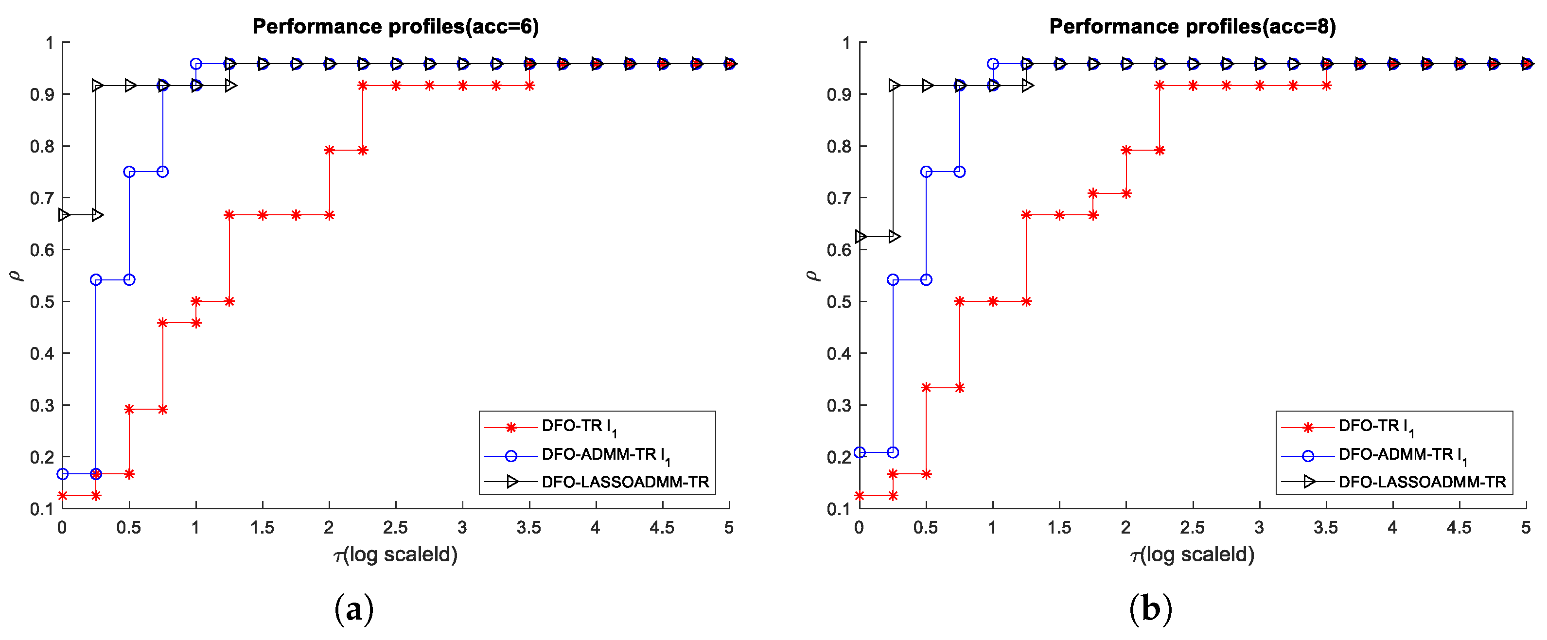
As for the performance profiles, in the numerical results, both in the cases of acc = 6 and acc = 8 , all functions except DIXMAANC reached the given accuracy. And Figure 2 illustrates the comparison results. It is worth noting that the ρ s ( τ ) values are plotted on a log-scale. In this context, ρ s ( 0 ) denotes the probability that a given algorithm is the best among all algorithms tested. Moreover, according to the definition of ρ s ( τ ) , in a certain sense, the smaller the τ (on a log-scale), the larger the ρ s ( τ ) , indicating that the algorithm can solve more problems.
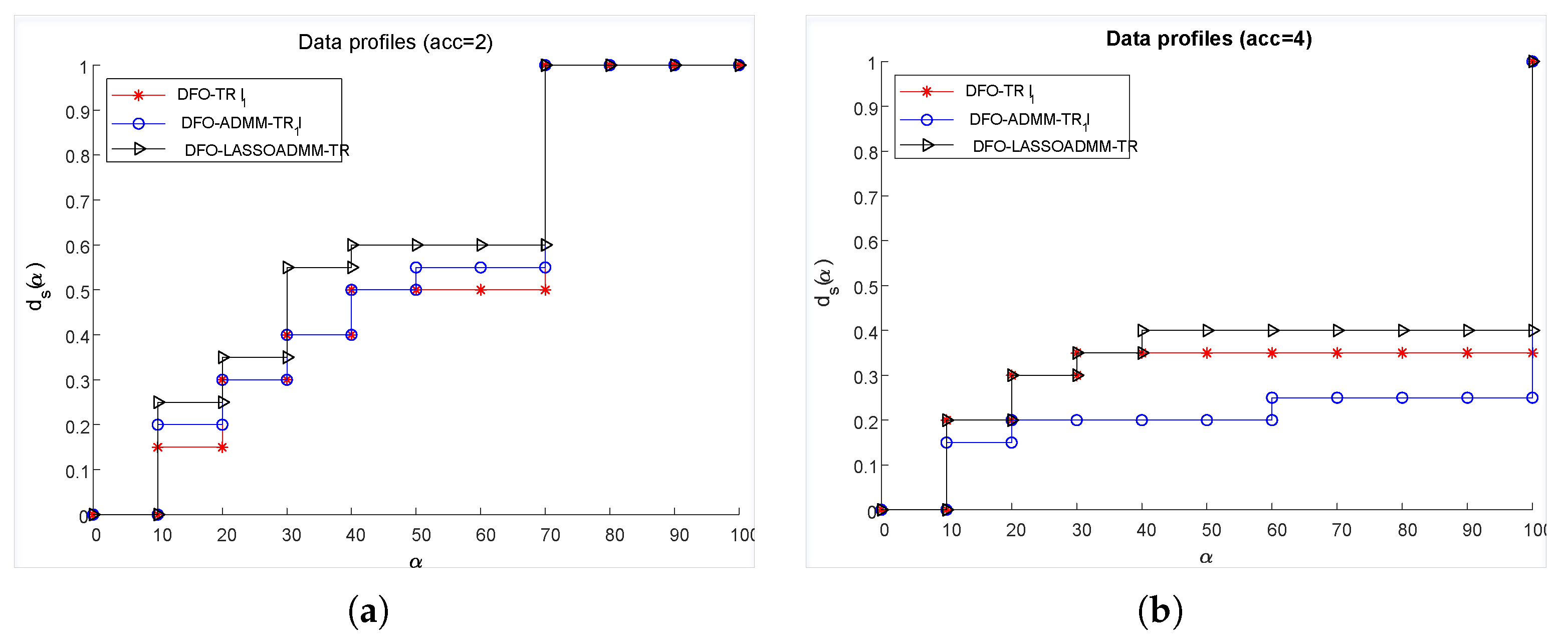
From Figure 2, it can be easily observed that, for both acc = 6 and acc = 8 , DFO-ADMM-TR l 1 and DFO-LASSOADMM-TR outperform DFO-TR l 1 . Figure 3 illustrates the comparison of the data profiles, and it can be reported that DFO-ADMM-TR l 1 performs better than the other two algorithms.
To be more specific, the following comprehensive conclusions can be deduced from Figure 2 and Figure 3: DFO-ADMM-TR l 1 demonstrates superiority over DFO-TR l 1 in both performance and data profiles, indicating the effectiveness of integrating ADMM into DFO-TR l 1 . In terms of performance profiles, the two proposed algorithms, DFO-ADMM-TR l 1 and DFO-LASSOADMM-TR, consistently outperform DFO-TR l 1 for both acc = 6 and acc = 8 , regardless of the value of τ . Furthermore, when examining data profiles, DFO-ADMM-TR l 1 is superior to the other two algorithms. It is understandable that DFO-LASSOADMM-TR might be inferior to DFO-TR l 1 because the accuracy of the surrogate model obtained by interpolation might be higher than that obtained by LASSO. However, adopting LASSO reduces the execution time of the algorithm, albeit at the cost of a slight increase in the number of function evaluations. Nevertheless, upon comparing Figure 2 and Figure 3, it is evident that DFO-ADMM-TR l 1 not only maintains its superiority but also significantly reduces the algorithm’s runtime, while the increase in the number of function evaluations is negligible.

4.3.2. Numerical Experiments for Noisy Case

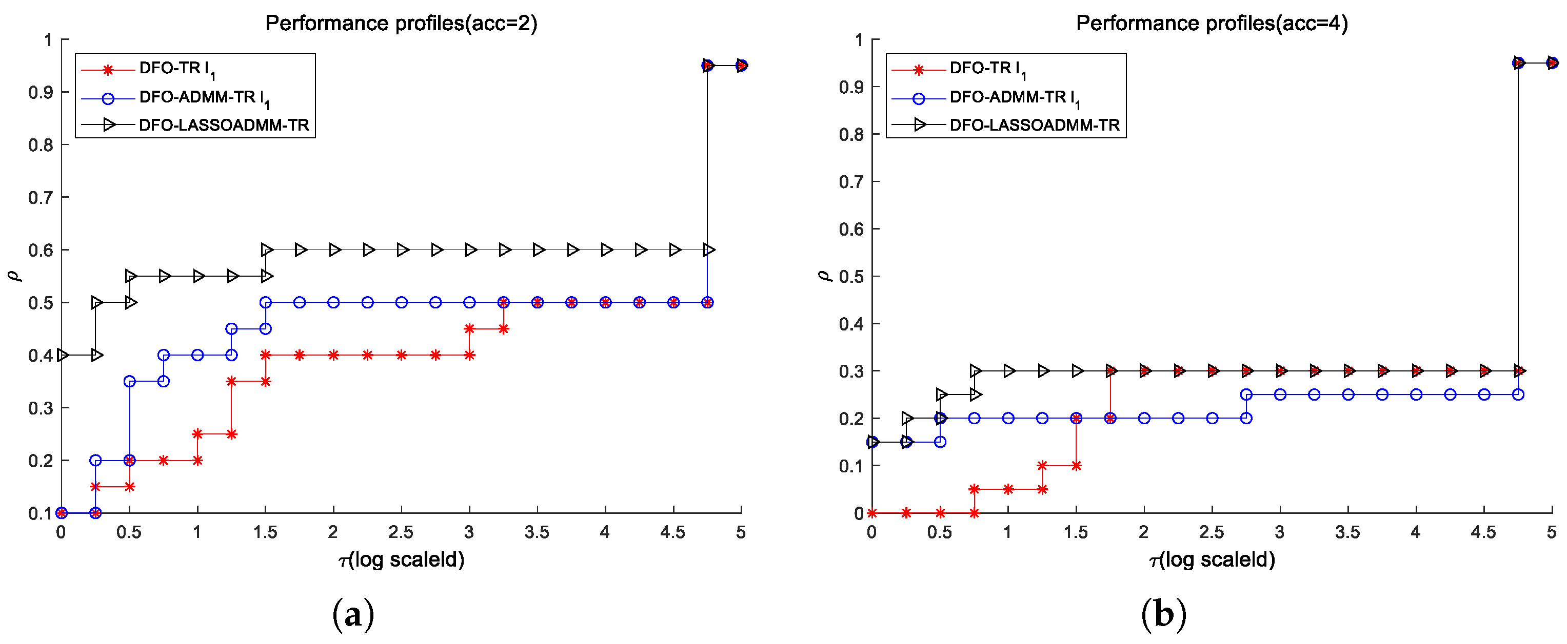
For the noisy optimization problems, we conduct numerical experiments in the same way as in the smooth case. However, for the performance profile, accuracy is set to acc = 2 and acc = 4 . Correspondingly, tolerance τ f is defined as τ f = 10 2 and τ f = 10 4 , respectively. Figure 4 and Figure 5 demonstrate that the application of the LASSO method enables the proposed DFO algorithm to attain enhanced performance, both in terms of performance profiles and data profiles.
As regards the size of the noise, taking the case acc = 2 as an example, Table 4 shows that adopting LASSO improves the algorithm’s ability to solve problems with noise. Besides, for a given accuracy, the proportion of problems that the algorithm can solve decreases as the size of the noise increases.
Overall, the proposed two algorithms are easy to adopt for solving problems with noise, particularly when LASSO is used to find the surrogate model. It is notable that the other proposed algorithm also benefits from the DFO-TR l 1 framework. The reason is that ADMM only converges to a modest accuracy, which is sufficient for many applications [33], making DFO-ADMM-TR l 1 more suitable for solving noisy problems. In conclusion, the numerical results provide a perspective for users solving optimization problems originating from practical applications. In other words, when the user needs to obtain the optimal solution as soon as possible, DFO-LASSOADMM-TR is a good choice. Moreover, DFO-LASSOADMM-TR is an alternative when there is noise in the problems.

5. Conclusions

In many practical industrial settings, one often encounters a type of optimization problem where the derivatives are hard to compute or unavailable. To address this issue, DFO methods have attracted the attention of researchers. Algorithms based on the surrogate model trust region framework constitute an important class of DFO methods. In this paper, we present two DFO algorithms that consider sparsity and noise, aiming to reduce computing time and decrease the number of function evaluations. One of the algorithms is an extension of the method proposed in [29]. Building on this, another algorithm is developed by integrating sparse modeling methods and interpolation techniques for constructing the surrogate model. Furthermore, in both algorithms, ADMM is applied to solve the optimization problem formulated for determining the coefficients of the surrogate models. Finally, the numerical experiments reported in this paper suggest that the proposed algorithms are both comparable and competitive.

Author Contributions

Conceptualization Y.L., Formal analysis Y.L., Funding acquisition Y.L., Investigation Y.L., Resources Y.L., Software Y.L., Visualization Y.L., Validation Y.L., Writing—original draft Y.L. and T.X., Writing—review & editing Y.L. and T.X. All authors have read and agreed to the published version of the manuscript.

Funding

This research is supported by the National Natural Science Foundation of China under Grant Nos. 62373204, 61977043, and the Talent Research Project Qilu University of Technology (Shandong Academy of Sciences) under Grant No. 2023RCKY159.

Data Availability Statement

The original contributions presented in the study are included in the article, further inquiries can be directed to the corresponding author.

Acknowledgments

Grateful acknowledgment is given to the editor and reviewers for their valuable insights and constructive feedback on our manuscript. Their expertise greatly contributed to enhancing the quality of our work.

Conflicts of Interest

The authors declare no conflicts of interest.

References

  1. Liu, C.; Tang, L.; Liu, J.; Tang, Z. A dynamic analytics method based on multistage modeling for a BOF steelmaking process. IEEE Trans. Autom. Sci. Eng. 2019, 16, 1097–1109. [Google Scholar] [CrossRef]
  2. Tang, L.; Meng, Y. Data analytics and optimization for smart industry. Front. Eng. Manag. 2020, 8, 157–171. [Google Scholar] [CrossRef]
  3. Feyzioglu, O.; Pierreval, H.; Deflandre, D. A simulation-based optimization approach to size manufacturing systems. Int. J. Prod. Res. 2005, 43, 247–266. [Google Scholar] [CrossRef]
  4. Coelho, G.F.; Pinto, L.R. Kriging-based simulation optimization: An emergency medical system application. J. Oper. Res. Soc. 2018, 69, 2006–2020. [Google Scholar] [CrossRef]
  5. Zhan, Z.H.; Zhang, J.; Li, Y.; Shi, Y.H. Orthogonal learning particle swarm optimization. IEEE Trans. Evol. Comput. 2011, 15, 832–847. [Google Scholar] [CrossRef]
  6. Srinivas, M.; Patnaik, L.M. Genetic algorithms: A survey. Computer 1994, 27, 17–26. [Google Scholar] [CrossRef]
  7. Du, K.L.; Swamy, M.N.S. Estimation of Distribution Algorithms. In Search and Optimization by Metaheuristics: Techniques and Algorithms Inspired by Nature; Springer International Publishing: Cham, Switzerland, 2016; pp. 105–119. [Google Scholar]
  8. Spendley, W.; Hex, G.R.; Himsworth, F.R. Sequential application for simplex designs in optimisation and evolutionary operation. Technometrics 1962, 4, 441–461. [Google Scholar] [CrossRef]
  9. Powell, M.J.D. An efficient method for finding the minimum of a function of several variables without calculating derivatives. Comput. J. 1964, 7, 155–162. [Google Scholar] [CrossRef]
  10. Conn, A.R.; Scheinberg, K.; Vicente, L. Introduction to Derivative-Free Optimization; Society for Industrial and Applied Mathematics: Philadelphia, PA, USA, 2009. [Google Scholar]
  11. Berahas, A.S.; Sohab, O.; Vicente, L.N. Full-low evaluation methods for derivative-free optimization. Optim. Methods Softw. 2023, 38, 386–411. [Google Scholar] [CrossRef]
  12. Gaudioso, M.; Liuzzi, G.; Lucidi, S. A clustering heuristic to improve a derivative-free algorithm for nonsmooth optimization. Optim. Lett. 2024, 18, 57–71. [Google Scholar] [CrossRef]
  13. Rios, L.M.; Sahinidis, N.V. Derivative-free optimization: A review of algorithms and comparison of software implementations. J. Glob. Optim. 2013, 56, 1247–1293. [Google Scholar] [CrossRef]
  14. Audet, C.; Hare, W. Derivative-Free and Blackbox Optimization; Springer: Cham, Switzerland, 2017. [Google Scholar]
  15. Gao, H.; Waechter, A.; Konstantinov, I.A.; Arturo, S.G.; Broadbelt, L.J. Application and comparison of derivative-free optimization algorithms to control and optimize free radical polymerization simulated using the kinetic Monte Carlo method. Comput. Chem. Eng. 2018, 108, 268–275. [Google Scholar] [CrossRef]
  16. Lucidi, S.; Maurici, M.; Paulon, L.; Rinaldi, F.; Roma, M. A derivative-free approach for a simulation-based optimization problem in healthcare. Optim. Lett. 2015, 10, 219–235. [Google Scholar] [CrossRef]
  17. Boukouvala, F.; Floudas, C.A. ARGONAUT: Algorithms for global optimization of constrained grey-box computational problems. Optim. Lett. 2017, 11, 895–913. [Google Scholar] [CrossRef]
  18. Boukouvala, F.; Hasan, M.M.F.; Floudas, C.A. Global optimization of general constrained grey-box models: New method and its application to constrained PDEs for pressure swing adsorption. J. Glob. Optim. 2017, 67, 3–42. [Google Scholar] [CrossRef]
  19. Liu, Y.; Tang, L.; Liu, C.; Su, L.; Wu, J. Black box operation optimization of basic oxygen furnace steelmaking process with derivative free optimization algorithm. Comput. Chem. Eng. 2021, 150, 107311. [Google Scholar] [CrossRef]
  20. Powell, M.J.D. On the global convergence of trust region algorithms for unconstrained minimization. Math. Program. 1984, 29, 297–303. [Google Scholar] [CrossRef]
  21. Conn, A.R.; Toint, P.L. An algorithm using quadratic interpolation for unconstrained derivative free optimization. In Nonlinear Optimization and Applications; Springer: Boston, MA, USA, 1996; pp. 27–47. [Google Scholar]
  22. Conn, A.R.; Scheinberg, K.; Toint, P.L. On the convergence of derivative-free methods for unconstrained optimization. In Approximation theory and optimization: Tributes to M. J. D. Powell; Iserles, A., Buhmann, M., Eds.; Cambridge University Press: Cambridge, UK, 1997; pp. 83–108. [Google Scholar]
  23. Sauer, T.; Xu, Y. On Multivariate Lagrange Interpolation. Math. Comput. 1995, 64, 1147–1170. [Google Scholar] [CrossRef]
  24. Powell, M.J.D. On trust region methods for unconstrained minimization without derivatives. Math. Program. 2003, 97, 605–623. [Google Scholar] [CrossRef]
  25. Conn, A.R.; Scheinberg, K.; Vicente, L.N. Geometry of interpolation sets in derivative free optimization. Math. Program. 2008, 111, 141–172. [Google Scholar] [CrossRef]
  26. Fasano, G.; Morales, J.L.; Nocedal, J. On the geometry phase in model-based algorithms for derivative-free optimization. Optim. Methods Softw. 2009, 24, 145–154. [Google Scholar] [CrossRef]
  27. Powell, M.J.D. The NEWUOA software for unconstrained optimization without derivatives. Large-Scale Nonlinear Optim. 2006, 83, 255–297. [Google Scholar]
  28. Scheinberg, K.; Toint, P.L. Self-correcting geometry in model-based algorithms for derivative-free unconstrained optimization. SIAM J. Optim. 2010, 20, 3512–3532. [Google Scholar] [CrossRef]
  29. Bandeira, A.S.; Scheinberg, K.; Vicente, L.N. Computation of sparse low degree interpolating polynomials and their application to derivative-free optimization. Math. Program. 2012, 134, 223–257. [Google Scholar] [CrossRef]
  30. Conn, A.R.; Scheinberg, K.; Vicente, L.N. Geometry of sample sets in derivative-free optimization: Polynomial regression and underdetermined interpolation. Ima J. Numer. Anal. 2008, 28, 721–748. [Google Scholar] [CrossRef]
  31. Foucart, S.; Rauhut, H. A Mathematical Introduction to Compressive Sensing; Birkhauser: New York, NY, USA, 2013. [Google Scholar]
  32. Tibshirani, R. Regression shrinkage and selection via the Lasso. J. R. Stat. Society. Ser. B (Methodol.) 1994, 58, 267–288. [Google Scholar] [CrossRef]
  33. Boyd, S.; Parikh, N.; Chu, E.; Peleato, B.; Eckstein, J. Distributed Optimization and Statistical Learning via the Alternating Direction Method of Multipliers; Now Foundations and Trends: Hanover, MA, USA, 2011. [Google Scholar]
  34. Yan, X.; Su, X. Linear Regression Analysis: Theory and Computing; World Scientific Publishing Co. Pte. Ltd.: Singapore, 2009. [Google Scholar]
  35. Rauhut, H. Compressive sensing and structured random matrices. Theor. Found. Numer. Methods Sparse Recovery 2010, 9, 1–92. [Google Scholar]
  36. Gould, N.I.M.; Orban, D.; Toint, P.L. CUTEr and SifDec: A constrained and unconstrained testing environment, revisited. ACM Trans. Math. Softw. 2003, 29, 373–394. [Google Scholar] [CrossRef]
  37. More, J.; Garbow, B.S.; Hillstrom, K.E. Testing unconstrained optimization software. ACM Trans. Math. Softw. 1981, 7, 17–41. [Google Scholar] [CrossRef]
  38. Conn, A.R.; Gould, N.I.M.; Lescrenier, M.J.A.; Toint, P.L. Performance of a multifrontal scheme for partially separable optimization. In Advances in Optimization and Numerical Analysis; Kluwer Academic Publishers: Dordrecht, The Netherlands, 1994; pp. 79–96. [Google Scholar]
  39. Buckley, A. Test Functions for Unconstrained Minimization; Dalhousie University: Halifax, NS, Canada, 1989. [Google Scholar]
  40. Toint, P.L. Test Problems for Partially Separable Optimization and Results for the Routine PSPMIN; Technology Report 83/4; Department of Mathematics, University of Namur: Brussels, Belgium, 1983. [Google Scholar]
  41. Fletcher, R. An optimal positive definite update for sparse hessian matrices. SIAM J. Optim. 1995, 5, 192–218. [Google Scholar] [CrossRef]
  42. Hansen, N.; Auger, A.; Finck, S.; Ros, R. Real-Parameter Black-Box Optimization Benchmarking 2010: Experimental Setup; Research Report; INRIA: Talence, France, 2010. [Google Scholar]
  43. Hock, W.; Schittkowski, K. Test Examples for Nonlinear Programming Codes; Springer: Berlin/Heidelberg, Germany, 1980; Volume 187. [Google Scholar]
  44. Dola, E.D.; More, J.J. Benchmarking optimization software with performance profiles. Math. Program. 2002, 91, 201–213. [Google Scholar] [CrossRef]
  45. More, J.J.; Wild, S.M. Benchmarking derivative-free optimization algorithms. SIAM J. Optim. 2009, 20, 172–191. [Google Scholar] [CrossRef]
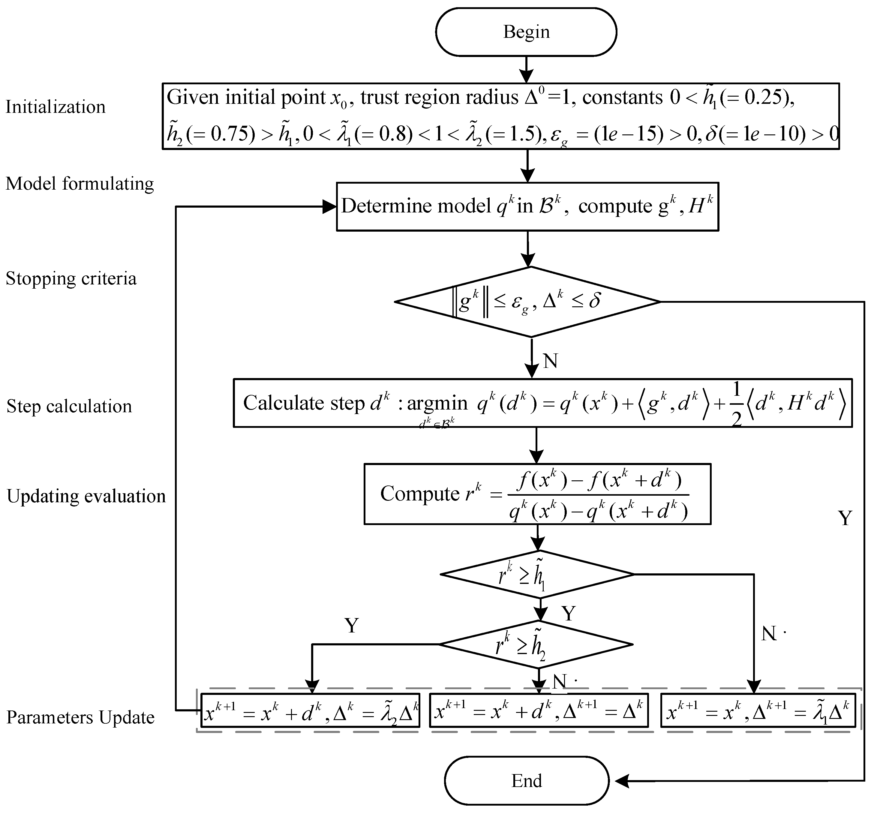
Figure 1. Flowchart of trust region algorithm.
Processes 12 02753 g001
Figure 2. Performance profiles compare between Algorithm DFO-TR l 1 , DFO-ADMM-TR l 1 and DFO-LASSOADMM-TR on smooth problems.
Processes 12 02753 g002
Figure 3. Data profiles compare between Algorithm DFO-TR l 1 , DFO-ADMM-TR l 1 and DFO-LASSOADMM-TR on smooth problems.
Processes 12 02753 g003
Figure 4. Performance profiles compare between Algorithm DFO-TR l 1 , DFO-ADMM-TR l 1 and DFO-LASSOADMM-TR on noisy problems.
Processes 12 02753 g004
Figure 5. Data profiles compare between Algorithm DFO-TR l 1 , DFO-ADMM-TR l 1 and DFO-LASSOADMM-TR on noise problems.
Processes 12 02753 g005
Table 1. Details of smooth problems.
ProblemSourse or Formula Formn
ARGLINB[37], Problem 3310
ARGLINC[37], Problem 348
ARWHEAD[38], Problem 5515
BDQRTIC[38], Problem 6110
BROYDN3DLS[37], Problem 3010
DIXMAANC[39], Page 4912
DIXMAANG[39], Page 4912
DIXMAANI[39], Page 4912
DIXMAANK[39], Page 4912
DIXON3DQ[39], Page 5112
DQDRTIC[40], Problem 2210
FLETCHCR[41], Problem 210
FREUROTH[37], Problem 210
GENHUMPS f 1 ( x ) 10
HIMMELBH[39], Page 602
MOREBVNE[39], Page 7510
NONDIA[39], Page 7610
NONDQUAR f 2 ( x ) 10
POWELLSG[37], Problem 134
POWER[39], Page 8318
ROSENBR[37], Problem 12
TRIDIA[40], Problem 810
VARDIM[37], Problem 2510
WOODS[37], Problem 144
Table 2. Details of noisy problems.
ProblemNoisen
Spheremoderate gaussian noise2, 4, 10
moderate uniform noise
severe gaussian noise2, 4
severe uniform noise
Rosenbrockmoderate gaussian noise2, 4, 10
moderate uniform noise
severe gaussian noise2, 4
severe uniform noise
Table 3. Run time(s) of the algorithm with different λ ^ L .
λ ^ L S0.00010.00050.0010.0050.010.050.10.51510
ARGLINB0.720.580.560.590.540.550.560.530.540.610.540.54
ARGLINC0.530.480.470.490.470.520.480.460.510.460.49
BDQRTIC1.571.421.571.261.461.201.321.311.641.33
DIXMAANC2.071.321.361.191.361.46
DIXMAANI2.260.920.820.97
DIXON3DQ0.840.640.670.700.500.960.940.760.77
DQDRTIC0.420.860.840.930.87
FREUROTH1.811.801.571.441.481.431.36
POWER0.830.800.840.820.830.750.790.750.800.88
TRIDIA0.630.730.710.700.570.670.75
Table 4. The percentage of problems solved by the algorithm.
DFO-TR l 1 DFO-TR l 1 DFO-LASSOADMM-TR
moderate noise58.33%58.33%75.00%
severe noise50.00%50.00%62.50%
Disclaimer/Publisher’s Note: The statements, opinions and data contained in all publications are solely those of the individual author(s) and contributor(s) and not of MDPI and/or the editor(s). MDPI and/or the editor(s) disclaim responsibility for any injury to people or property resulting from any ideas, methods, instructions or products referred to in the content.