Hierarchical Power System Scheduling and Energy Storage Planning Method Considering Heavy Load Rate

Abstract

With the rise in the proportion of renewable energy and energy storage in modern power systems, the volatility of renewable energy and the increasing demand for loads pose a significant risk of congestion in transmission lines. Along with transmission congestion, prolonged heavy loads on transmission lines increase equipment failure rates, leading to a range of issues within the power system. This study proposes a scene clustering method for power system scheduling by leveraging the net load related with the load and renewable energy power outputs. Subsequently, a scheduling model and line load evaluation indexes were developed to analyze the line load rate of power systems with different renewable energy proportions. The simulation results indicate that the utilization rate of lines, the fluctuation rate of line load, the maximum line load, and heavy line load time increase as the installed proportion of renewable energy increases. Finally, a penalty term for heavy loads was incorporated into the objective function and methods of rescheduling and planning energy storage considering the heavy load penalty function are proposed. A case study validated the significant improvements in load management, achieving a reduction in heavy load time by approximately 30% and reducing transmission congestion by 20% under high-renewable-energy-penetration scenarios. These results illustrate the effectiveness of the heavy load cost function in enhancing system resilience and optimizing load distribution.

1. Introduction

In the past few decades, many countries have implemented policies to develop renewable energy (RE) to reduce carbon emissions and combat global climate change. According to the International Energy Agency’s forecast, renewables have a strong chance of surpassing the installed capacity of traditional power sources by 2027. However, the fluctuating and intermittent nature of RE introduces several challenges to power systems, including a decreased reliability of electrical supplies. As renewable energy penetration accelerates, electricity transmission issues become more complex. The fluctuation in renewable energy and the variability in dispatch operation scenarios increase the probability of transmission line overloading [1].

In engineering practice, the overloading of transmission lines will have a greater impact on the safety and stability of the power system, which is an event that should be avoided in the operation of the power system. In addition, transmission line heavy load (TLHL) is also a matter of key concern. The long-term heavy load operation of transmission lines will reduce its service life and lead to performance degradation [2]. Similarly, Ref. [3] indicated that prolonged heavy loads on transmission and transformation equipment increases the likelihood of fatigue damage. Ref. [4] researched the relationship between the load rates of power system components and the self-organized critical status of the power system, finding that reducing the load rate of heavily loaded components can effectively decrease the probability of large-scale cascading failures. In power systems with high renewable energy penetration, the uncertainty of power flow due to substantial renewable energy input increases the risk of damage to power equipment. Consequently, some power grid companies in China are required to limit the number of heavy load lines with load rates exceeding 80% [5].

Although the TLHL has been assessed in practical engineering, it is rarely integrated with the constraints of heavy load and transmission line capacity in scheduling optimization. Most scheduling methods focus solely on transmission line capacity [6,7,8]. However, if TLHL is not considered in scheduling, the fluctuating output of increasing renewable energy may make it more difficult to achieve the goal of limiting the number of heavily loaded lines. Addressing TLHL through transmission line expansion or by reducing transmission line utilization would increase transmission costs. Therefore, it is essential to consider both TLHL and transmission capacity limits during scheduling. Additionally, reducing the duration of TLHL can help lower the probability of transmission congestion, providing a buffer of surplus transmission capacity against intermittent congestion caused by fluctuating renewable energy and ultimately saving on transmission line expansion investments [9].

In addition to scheduling, transmission capacity including overload and TLHL issues is one of the important constraints in power system planning [10]. The planning in the power system includes generation expansion planning (GEP) [11], transmission expansion planning (TEP) [12], energy storage planning (ESP) [13], and so on [14]. However, TLHL has not been considered in conventional planning. Taking TLHL into account in planning would enhance scheduling efficiency through a more appropriate site and capacity selection of planned objects, thereby mitigating risk in scheduling.

With the rapid development of energy storage [15] in recent years, independent ESP without GEP and TEP has become increasingly popular. On the one hand, the increase in renewable energy power supply brings about a significant demand for power regulation. On the other hand, many social investors are willing to invest money in energy storage projects building energy storage power stations in the situation that energy storage systems can profit through participating in the ancillary services market with policy incentives [16]. Long-term planning for energy storage mainly provides auxiliary support for the power system by adjusting the power shortage or surplus caused by fluctuations in load and RE output rather than keeping the transmission lines working perfectly [14,17]. ESP with a TLHL constraint could provide a larger space for electricity transmission without other excess investments to minimize the transmission restriction of the energy storage transmission section.

Despite advancements in power system scheduling and ESP, the integration of high levels of RE introduces significant challenges due to its variability and unpredictability. Traditional scheduling models often overlook the issue of TLHL, which arises from increased RE penetration. Persistent heavy load conditions lead to congestion and accelerated infrastructure wear, yet existing methods primarily focus on minimizing costs and general load balancing without specific TLHL considerations. Previous research has given less consideration to the role of energy storage in the operation scheduling and planning of power system transmission line heavy load issues. This study fully explores the role of energy storage in power system energy regulation and proposes a scheduling model and line load assessment indicators to analyze the line load rate of power systems with different proportions of renewable energy. A detailed comparison is shown in

Table 1. Research comparison.

Study	Focus Area	Advantages	Limitations	Improvements
[1,2,3]	Distribution network scheduling and energy storage planning	Enhances flexibility, reduces RE curtailment	Limited focus on sustained heavy loads	Integrates energy storage planning with LLR
[4,5,6]	Multi-objective load management	Balances cost and load, effective for short-term overloads	Limited adaptation to prolonged heavy load conditions	Adds a heavy load penalty to improve resilience under sustained high loads
[7,8,9]	Hybrid energy storage and RE integration	Reduces RE waste, improves economic efficiency	Lacks line-specific heavy load management	Uses scenario clustering and load penalties for stability in high-RE scenarios
[10,11,12]	RE variability and dynamic dispatch	Supports stability with RE variability and market	Limited to short-term scenarios, lacks sustained load solutions	Adapts to RE variability using scenario clustering and heavy load penalties
[13,14,15]	Transmission load balancing and grid stability	Manages peak loads, prevents overloads	Focused on immediate congestion, lacks long-term load management	Mitigates cumulative heavy loads with continuous heavy load penalty
[16,17]	RE integration with demand response and grid resilience	Increases flexibility under RE conditions	Lacks tools for managing sustained heavy loads	Introduces multi-layered penalty to enhance resilience under high RE

.

In response to the current issue of the insufficient consideration of TLHL in the optimization and planning of power system dispatch, this paper studies the transmission line load rate of power systems with renewable energy, incorporating the maximum transmission capacity and TLHL into the system’s dispatch optimization and planning. It is reflected in the objective function in the form of a line overload penalty function and reasonably plans energy storage to fully leverage the system regulation capabilities of energy storage to address the TLHL issues in power systems. The contributions of this paper are summarized as follows:

(1)

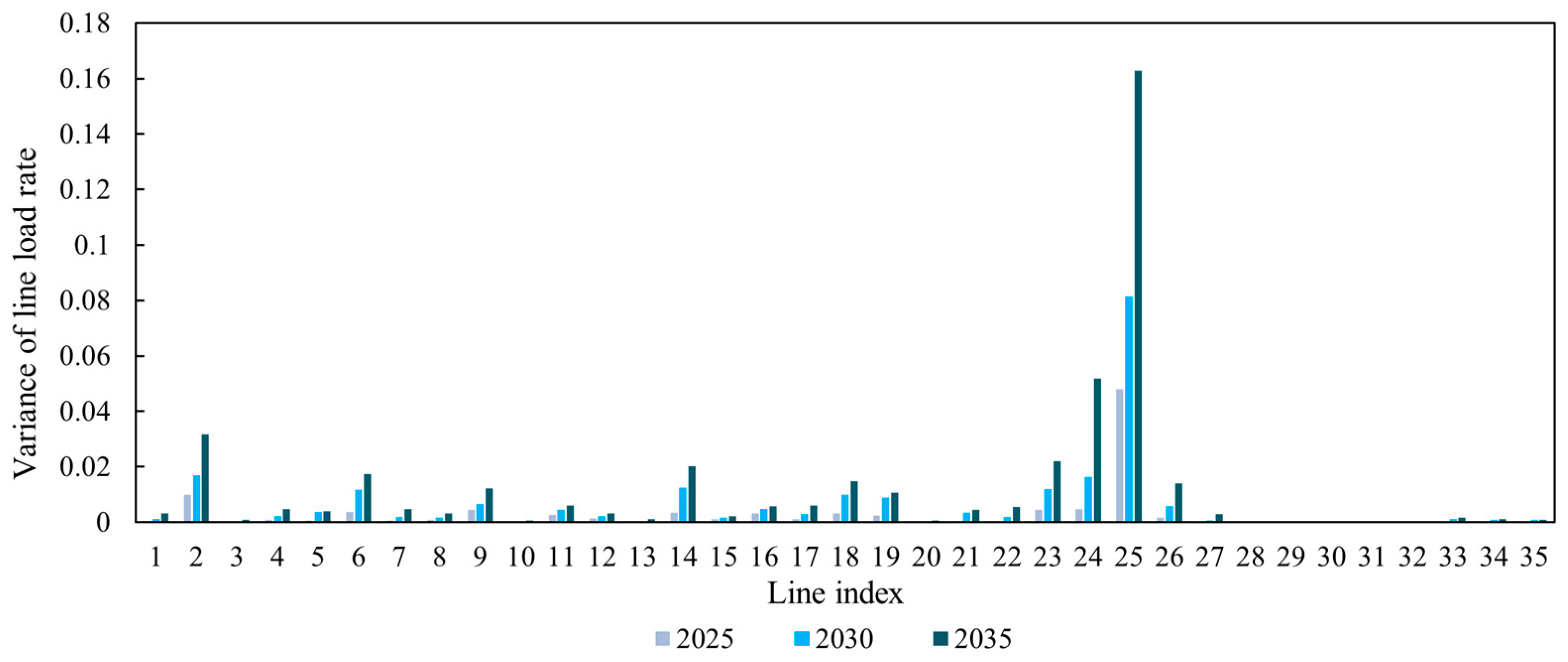
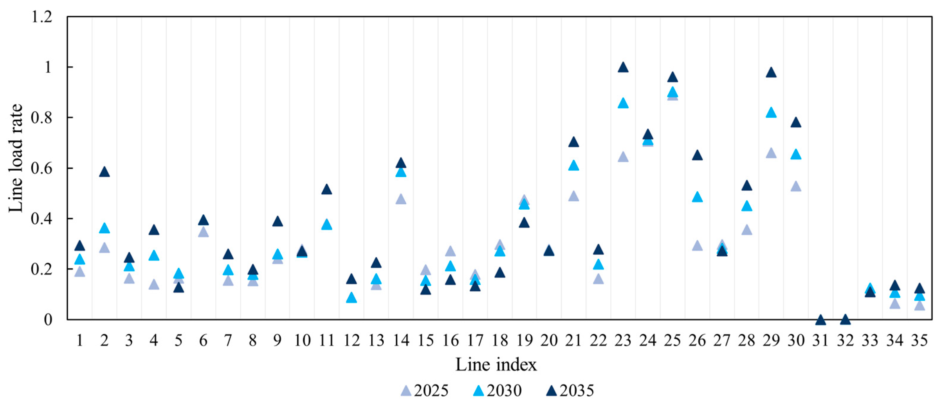
Dimensionless indicators are proposed to evaluate the impact of renewable energy on transmission line load and illustrate high-risk lines’ TLHL. By simulating scheduling operations, the increasingly serious problem of TLHL in a power system with an increasing proportion of renewable energy but an unchanged transmission network is pointed out.

(2)

Compared to conventional scheduling and ESP methods, the ESP–scheduling integrated model considering both maximum transmission capacity and TLHL are proposed to enhance operational security and economic benefits.

(3)

Finally, a penalty term for heavy loads was incorporated into the objective function and methods of rescheduling and planning energy storage considering the heavy load penalty function are proposed. The dispatching layer outputs the system operation data, and the planning layer conducts energy storage planning based on the operational data.

The remaining of this paper is organized as follows: Section 2 demonstrates the scene clustering method, scheduling models, planning models, and indexes of line load. Section 3 provides an analytical example and verifies the effectiveness of the proposed model. Section 4 summarizes all the work and analysis results of this study.

2. Problem Formulation and Model Construction

2.1. Scenario Construction and Renewable Energy Output Models

Due to the variability in power system dispatch caused by fluctuations in renewable energy (RE) output, traditional research methods that focus on single or few dispatch scenarios are no longer representative as the proportion of RE in the power system increases. The net load, which is the remaining electricity demand after accounting for renewable energy generation, effectively describes the actual electricity demand of the power grid. One of the grid’s primary objectives is to fully utilize renewable energy generation. Therefore, the typical scenarios for scheduling and planning in this paper are based on net load.

The net load in the power system can be calculated using Equation (1).

$$D_{L-RE,t}={\displaystyle \sum _{b\in B}P{L}_{b,t}}-{\displaystyle \sum _{g_{re}\in G_{re}}{P}_{re,g_{re},t}^{\prime }}$$

(1)

where $D_{L-RE,t}$ represents the net load at the $t^{th}$ time (MW); $P{L}_{b,t}$ is the sum of all buses’ loads at the $t^{th}$ time (MW); and $P_{re,g_{re},t}^{\prime }$ is the sum of all RE units’ power outputs at the $t^{th}$ time (MW).

The scene is divided into general scenarios clustered by the k-means clustering algorithm using every day’s net load and extreme scenarios with the maximum and minimum net load. The maximum and minimum net load days are determined by calculating the daily total net load values, as shown in Equations (2) and (3).

$$D{’}_{L-RE,\max }=\mathrm{MAX}{\left({\displaystyle \sum _{t\in T}{D}_{L-RE,t}}\right)}_d$$

(2)

$$D{’}_{L-RE,\min }=\mathrm{MIN}{\left({\displaystyle \sum _{t\in T}{D}_{L-RE,t}}\right)}_d$$

(3)

where $D{’}_{L-RE,\max }$ represents the maximum net load of the $d^{th}$ day (MW) and $D{’}_{L-RE,\min }$ represents the minimum net load of the $d^{th}$ day (MW).

In this study, the k-means clustering algorithm is used to classify typical net load scenarios, which are influenced by RE variability and fluctuating power demands. The choice of k-means clustering is motivated by its simplicity, efficiency, and suitability for large datasets, making it well suited for our power system data, which include daily load profiles across multiple scenarios. K-means clustering minimizes the variance within each cluster, allowing us to group days with similar net load patterns, which is crucial for accurately capturing the operational variability in RE output and demand. The basic principle of the K-means clustering algorithm is as follows:

The k-means algorithm is an iterative solution of the cluster analysis algorithm; its core idea is to divide n objects in the dataset into k clusters, so that each object to the center of the cluster to which it belongs (or known as the mean point, the center of mass) of the sum of the distances is minimum, which is shown in the Figure 1.

The execution process of the k-means algorithm usually includes the following steps (Figure 1):

(1)

Initialization: selection of k initial clustering centers.

At the beginning of the algorithm, k data points need to be randomly selected as the initial clustering centers.

(2)

Assignment: assign each data point to the nearest clustering center.

For each data point in the dataset, calculate its distance from each clustering center and assign it to the cluster center with the closest distance.

(3)

Update: recalculate the center of each cluster.

For each cluster, recalculate its cluster center. The new cluster center is the mean of all data points within that cluster.

(4)

Iterate: repeat the allocation and update steps until the termination condition is met.

Repeat the assignment and update steps until the cluster centers no longer change significantly. A key advantage of k-means clustering in this context is its iterative approach to minimizing intra-cluster variance, which enhances the model’s accuracy in identifying patterns in RE variability and load fluctuation. Compared to alternative clustering methods, k-means offers a balanced trade-off between computational efficiency and clustering precision, allowing for its practical application in large-scale systems.

The renewable energy generation values are obtained from a calculation utilizing the meteorological data and renewable energy output models.

As shown in Equation (4), the output of wind turbines, including the rate power, cut-in wind speed, rated wind speed, and cut-out wind speed, can be obtained from the basic performance parameters of wind turbines installed in wind farms.

$$P_{\mathrm{W}}\left(v\right)=\left\{\begin{array}{l}0,\hfill \\ c_{1}v+c_2,\hfill \\ P_{\mathrm{N}},\hfill \end{array}\right. \begin{array}{l}v\le v_{\mathrm{ci}} \mathrm{or} v\ge v_{\mathrm{co}}\hfill \\ v_{\mathrm{ci}}\le v\le v_{\mathrm{r}}\hfill \\ v_{\mathrm{r}}\le v<v_{\mathrm{co}}\hfill \end{array}$$

(4)

where $P_{\mathrm{W}}\left(v\right)$ indicates the relationship between the wind turbine active output $P_{\mathrm{W}}$ (MW) and wind speed $v$ (m/s); $v_{\mathrm{ci}}$, $v_{\mathrm{co}}$, and $v_{\mathrm{r}}$ represent the cut-in, cut-out, and rated wind speed of the wind turbine, respectively (MW); $c_1$ and $c_2$ are wind turbine output characteristic curve coefficients; and $P_{\mathrm{N}}$ is the rated power of the wind turbine (MW).

Since the active output of solar power is proportional to the radiant intensity, solar power generation is generally described by a beta distribution [18]. The relationship between the radiant intensity and active output of solar power generation is shown in Equation (5).

$$P_{\mathrm{PV}}(r)=\left\{\begin{array}{ll}{N}_{\mathrm{PV}}{P}_{\mathrm{rs}}\times \left({\displaystyle \frac{r^2}{R_{\mathrm{STD}}{R}_{\mathrm{C}}}}\right),\hfill & 0\le r\le R_{\mathrm{C}}\\ N_{\mathrm{PV}}{P}_{\mathrm{rs}}{\displaystyle \frac{r}{R_{\mathrm{STD}}{R}_{\mathrm{C}}}},\hfill & R_{\mathrm{C}}\le r\le R_{\mathrm{STD}}\\ N_{\mathrm{PV}}{P}_{\mathrm{rs}},\hfill & r\ge R_{\mathrm{STD}}\end{array}\right.$$

(5)

where $P_{\mathrm{PV}}(r)$ indicates the relationship between the solar system output $P_{\mathrm{PV}}$ (MW) and solar radiation intensity $r$ (W/m²); $N_{\mathrm{PV}}$ is the number of photovoltaic units; $P_{\mathrm{rs}}$ is the rated power of the photovoltaic unit (MW); $R_{\mathrm{STD}}$ is the standard solar radiation (usually 1000 W/m²); and $R_{\mathrm{C}}$ is the radiant (usually 150 W/m²).

2.2. Scheduling Optimization Model

2.2.1. Scheduling Objective Function

In numerous studies on the optimal scheduling of power systems containing RE, the most common approach combines power system cost minimization with other objective functions. Therefore, in this study, a direct current power flow model has been established, where one of the main optimization objectives is minimizing the operating cost of the power system, assuming a fixed construction cost. The efficient utilization of RE electricity promotes the development of renewable energy and supports the low-carbon operation of the power system. Thus, minimizing the waste of RE electricity is also a key objective. In addition, a penalty function for the line heavy load rate exceeding the secure value was added to the objective function. Equation (6) is the objective function containing the first two, which means that the objective of the heavy load is not considered, whereas Equation (7) involves all these objectives and the penalty function. The details of each objective and the penalty function are shown in Equations (8)–(11). It should be noted that the penalty term is the difference between the actual line load rate (LLR) and the required heavy load rate, as Equation (10) shows. The penalty factor discourages heavy load conditions by applying a cost whenever transmission line loads exceed a set threshold (e.g., 80% of capacity). The penalty increases proportionally with load beyond this threshold, which can be adjusted linearly or nonlinearly (e.g., quadratic scaling) to apply higher penalties as the load approaches full capacity. This factor, integrated into the objective function, incentivizes the model to favor load-balancing and congestion-mitigating strategies, enhancing system resilience under high renewable energy integration.

$$\mathrm{Objective}{’}_{\mathrm{operation}}=\mathrm{MIN}\left(a_1\times O_{\mathrm{cost}}+a_2\times O_{\Delta \mathrm{re}}\right)$$

(6)

$${\mathrm{Objective}}_{\mathrm{operation}}=\mathrm{MIN}\left(a_1\times O_{\mathrm{cost}}+a_2\times O_{\Delta \mathrm{re}}+F\left(f_l(P_{g,t}),\alpha \right)\right)$$

(7)

$$O_{cost}={\displaystyle \sum _{t\in T}{\displaystyle \sum _{g\in G}(P_{g,t}\times F_{\mathrm{operation}}+\left|N_{g,t}-N_{g,t-1}\right|\times F_{\mathrm{on}-\mathrm{off},g})}+{\displaystyle \sum _{i\in I}{P}_{\mathrm{ex},i,t}\times F_{\mathrm{ex},i}}}$$

(8)

$$O_{\Delta re}={\displaystyle \sum _{t\in T}{\displaystyle \sum _{g_{\mathrm{re}}\in G_{re}}\left|P_{\mathrm{re},g_{\mathrm{re}},t}^{\prime }-P_{\mathrm{re},g_{\mathrm{re}},t}\right|}}$$

(9)

$$f_l\left(P_{g,t}\right)=\left\{\begin{array}{ll}0,\hfill & \left|{\displaystyle \frac{{\displaystyle \sum _{g\in G}\left(P_{g,t}\times PTD{F}_l\right)}}{C_l}}\right|\le c_{\mathrm{hl}};\hfill \\ \left|{\displaystyle \frac{{\displaystyle \sum _{g\in G}\left(P_{g,t}\times PTD{F}_l\right)}}{C_l}}\right|-c_{\mathrm{hl}},\hfill & \left|{\displaystyle \frac{{\displaystyle \sum _{g\in G}\left(P_{g,t}\times PTD{F}_l\right)}}{C_l}}\right|>c_{\mathrm{hl}}\hfill \end{array}\right.$$

(10)

$$F\left(f_l(P_{g,t}),\alpha \right)=\alpha \times {\displaystyle \sum _{l\in L}{f}_l\left(P_{g,t}\right)}$$

(11)

where $\mathrm{Objective}{’}_{\mathrm{operation}}$ and $\mathrm{Objective}{e}_{\mathrm{operation}}$ are scheduling objective functions without and with the consideration of the penalty of heavy loads, respectively; $O_{\mathrm{cost}}$ and $O_{\Delta \mathrm{re}}$ represent the economic objective function and abandoned amount of RE objective function; $F\left(f_l(P_{g,t}),\alpha \right)$ is penalty function of a heavy load line; $f_l(P_{g,t})$ is the exceeding value of the heavy load rate of the $l^{th}$ line; $\alpha$ is the penalty factor of line heavy load; $a_1$ and $a_2$ are optimization objective weight coefficients; $P_{g,t}$ is the power of the $g^{th}$ generator at the $t^{th}$ time (MW); $N_{g,t}$ and $N_{g,t-1}$ are binary variables on the status of the $g^{th}$ generator at the $t^{th}$ time and the ${(t-1)}^{th}$ time; $P_{\mathrm{ex},i,t}$ is the external power of the $i^{th}$ power source at the $t^{th}$ time (MW); $F_{\mathrm{operation},g}$, $F_{\mathrm{on}-\mathrm{off},g}$, and $F_{\mathrm{ex},i}$ are the operating cost of the $g^{th}$ generator (¥/MW), operating cost the $g^{th}$ generator (¥/MW), and the external power cost of the $i^{th}$ source (¥/MW), respectively; $P_{\mathrm{re},g_{re},t}’$ and $P_{\mathrm{re},g_{re},t}$ represent the power output calculated based on meteorological data of the $g_{re}^{th}$ RE generator at the $t^{th}$ time (MW) and the power output of the $g_{re}^{th}$ RE generator at the $t^{th}$ time (MW), respectively; $PTD{F}_l$ is the power transfer distribution factor at the $l^{th}$ line; $C_l$ is the transmission capacity at the $l^{th}$ line (MW); and $c_{\mathrm{hl}}$ is the heavy load rate required by the power system (usually 80%).

2.2.2. Constraints for Scheduling

The stability, risk resistance, nature of various power sources, and transmission network constraints of the scheduling optimization model include the power balance with Equation (12), system reserve capacity with Equations (13) and (14), generator unit performance with Equations (15) and (16), incoming electricity quota with Equation (17), energy storage restrictions with Equations (18)–(20), and the transmission capacity limit with Equation (21).

Power demand and supply balance should be ensured at every moment as follows:

$${\displaystyle \sum _{g\in G}{P}_{g,t}}+{\displaystyle \sum _{i\in I_{\mathrm{ex}}}{P}_{\mathrm{ex},i,t}}={\displaystyle \sum _{b\in B}P{L}_{b,t}}$$

(12)

The constraints of system reserve capacity include the spinning reserve capacity supplied by the running units, with quickly responsive adjustment capacity such as adjustable in-service hydroelectric units and non-spinning reserve capacity provided by the quick-startup power units with shutdown status.

$${\displaystyle \sum _{g_{\mathrm{sr}}\in G_{\mathrm{sr}}}\left(C_{g_{\mathrm{sr}}}\times N_{g_{\mathrm{sr}},t}-P_{g_{\mathrm{sr}},t}\right)}\ge c_{\mathrm{sr}}\times P{L}_{\max }$$

(13)

$${\displaystyle \sum _{g_{\mathrm{nsr}}\in G_{\mathrm{nsr}}}\left(C_{g_{\mathrm{nsr}}}\times (1-N_{g_{\mathrm{nsr}},t})\right)}\ge c_{\mathrm{nsr}}\times P{L}_{\max }$$

(14)

where $C_{g_{\mathrm{sr}}}$ and $C_{g_{\mathrm{nsr}}}$ are the capacity of the $g_{\mathrm{sr}}^{th}$ spinning reserve generator (MW) and capacity of the $g_{\mathrm{nsr}}^{th}$ non-spinning reserve generator (MW), respectively; $c_{\mathrm{sr}}$ and $c_{\mathrm{nsr}}$ are ratios of the spinning reserve and non-spinning reserve to load; $N_{g_{\mathrm{sr}},t}$ and $N_{g_{\mathrm{nsr}},t}$ are binary variables on the status of the $g_{\mathrm{sr}}^{th}$ spinning reserve generator and the $g_{\mathrm{nsr}}^{th}$ non-spinning reserve generator at the $t^{th}$ time, respectively; $P_{g_{\mathrm{sr}},t}$ is the power of the $g_{\mathrm{sr}}^{th}$ spinning reserve generator at the $t^{th}$ time (MW); and $P{L}_{\max }$ is the maximum load of the power system (MW).

Limitations on unit capacity and the power output change rate are the most important indicators in generator unit performance (including the units of energy storage) when simulating the scheduling operation of a power system; therefore, these two constraints are considered in the scheduling model.

$$P_{\min ,g}\le P_{g,t}\le P_{\max ,g}$$

(15)

$$-P_{\mathrm{down},g}\le P_{g,t}-P_{g,t-1}\le P_{\mathrm{up},g}$$

(16)

where $P_{\min ,g}$ and $P_{\max ,g}$ are the minimum and maximum power of the $g^{th}$ generator (MW); $P_{\mathrm{down},g}$ and $P_{\mathrm{up},g}$ are speeds of power reduction and power increase in the $g^{th}$ generator (MW/h).

The external power supply is set as a power supply that can be scheduled and adjusted within the full power range.

$$0\le P_{\mathrm{ex},i,t}\le C_{\mathrm{ex},i}$$

(17)

where $C_{ex,i}$ is the external power capacity of the $i^{th}$ power source (MW).

Besides power capacity and the output change rate, there are other constraints on energy storage, such as the energy capacity and charge/discharge cycles.

$$0\le E_{s,g_s,t}\le C{E}_{s,g_s}$$

(18)

$$0\le E_{s,g_s,t-1}-{\displaystyle \frac{P_{g_s,t}}{ef{f}_{P,g_s}}}+C{h}_{g_s,t}\times ef{f}_{Ch,g_s}\le C{E}_{s,g_s}$$

(19)

$${\displaystyle \sum _{t\in T}{P}_{g_s,t}}={\displaystyle \sum _{t\in T}C{h}_{g_s,t}}$$

(20)

where $E_{s,g_s,t}$ is the remaining dischargeable energy of the $g_s^{th}$ energy storage at the $t^{th}$ time (MWh); $C{E}_{s,g_s}$ is the energy capacity of the $g_s^{th}$ energy storage (MWh); $P_{g_s,t}$ and $C{h}_{g_s,t}$ represent the dischargeable power and chargeable power of the $g_s^{th}$ energy storage at the $t^{th}$ time, respectively (MW); and $ef{f}_{P,g_s}$ and $ef{f}_{Ch,g_s}$ are the discharge efficiency and charge efficiency of the $g_s^{th}$ energy storage.

The last of the scheduling constraints is the line capacity limit, whose actual transmission line loads are calculated by the power transfer distribution factor.

$$-C_l\le {\displaystyle \sum _{g\in G}\left(P_{g,t}\times PTD{F}_l\right)}\le C_l$$

(21)

2.3. Energy Storage Planning Model

The energy storage planning method for alleviating congestion and line heavy load is based on the energy storage planning model, considering the geographical conditions where the better places for installing energy storage systems are and the planned energy storage performance parameters. When the capacity of the planned energy storage is regarded as a variable, the energy storage planning model is established by adding additional variables, objectives, and constraints based on the above scheduling optimization model to adapt the set scheduling rules. The scheduling model focuses on optimizing day-to-day operations, ensuring efficient power distribution while minimizing renewable energy curtailment and operational costs. By incorporating a heavy load cost function, this model helps avoid line overloads in real time. The planning model, in turn, uses data from the scheduling model—such as trends in load and congestion patterns—to make long-term infrastructure decisions, especially in siting and sizing energy storage systems. The heavy load cost in the planning model signals areas where new storage would be most beneficial for reducing chronic overloads. This integration enables both short-term efficiency and long-term resilience, aligning real-time adjustments with strategic infrastructure development.

2.3.1. Planning Objective Function

It is necessary to build a new energy storage system with fewer expenses to enable the practical application of the planning results; therefore, the objective of minimizing the planned energy storage construction costs has been considered in the objective function. For the planning goal of reducing the line heavy load, the newly planned energy storage on each bus is required to adjust locally as much as possible to limit excessive power transmission; hence, the penalty function is maintained in the objective function. Combining the economical and environmentally friendly requirements for power system scheduling, the objectives of the energy storage planning model are described by Equations (22) and (23) as follows:

$${\mathrm{Objective}}_{\mathrm{plan}}=\mathrm{MIN}\left(a_3\times O_{\mathrm{cost}}+a_4\times O_{\Delta \mathrm{re}}+a_5{O}_{\mathrm{plan}\_\mathrm{cost}}+F\left(f_l(P_{g,t}),\alpha \right)\right)$$

(22)

$$O_{\mathrm{plan}\_\mathrm{cost}}={\displaystyle \sum _{m\in M}{C}_{\mathrm{plan},m}\times F_{\mathrm{storage},m}}$$

(23)

where $O_{\mathrm{plan}\_\mathrm{cost}}$ is the cost objective function for planning energy storage; $C_{\mathrm{plan},m}$ is the capacity of the $m^{th}$ energy storage (MW); $a_3$, $a_4$, and $a_5$ are planning optimization objective weight coefficients; and $F_{\mathrm{storage},m}$ is the cost of construction of the $m^{th}$ planning energy storage (¥/MW).

The objective of another planning model without a heavy load penalty function is expressed in Equation (24).

$$\mathrm{Objective}{’}_{\mathrm{plan}}=\mathrm{MIN}\left(a_3\times O_{\mathrm{cost}}+a_4\times O_{\Delta \mathrm{re}}+a_5{O}_{\mathrm{plan}\_\mathrm{cost}}\right)$$

(24)

2.3.2. Constraints for Planning

Because some constraints in the scheduling model are related to energy storage units, such as the power balance constraint and line transmission capacity limit, the planned energy storage must also meet these constraints. The planning variables and parameters added to the original energy storage unit were $P_{g_{\mathrm{s}},plan,t}$, $C{h}_{g_{\mathrm{s}},\mathrm{plan},t}$, $E_{\mathrm{s},g_{\mathrm{s}},\mathrm{plan},t}$, $E_{\mathrm{s},g_{\mathrm{s}},\mathrm{plan},t-1}$, $C{E}_{\mathrm{s},g_{\mathrm{s}},\mathrm{plan}}$, $ef{f}_{\mathrm{P},g_{\mathrm{s}},\mathrm{plan}}$, and $ef{f}_{\mathrm{Ch},g_{\mathrm{s}},\mathrm{plan}}$. Moreover, the planned capacity of various types of energy storage should be limited based on the geographical and total amount conditions at different nodes, as shown in Equations (25) and (26). Equation (25) represents the constraints for energy storage planning at the bus, and Equation (26) represents the constraints for the total energy storage capacity. For example, the construction of pumped storage hydroelectricity requires sufficient water around the terrain with a relatively large height difference.

$$C_{\mathrm{plan},\min ,b}\le {\displaystyle \sum _{m_{\mathrm{b}}\in M_{\mathrm{b}}}{C}_{\mathrm{plan},m_{\mathrm{b}},b}}\le C_{\mathrm{plan},\max ,b}$$

(25)

$$C_{\mathrm{plan},\min ,m}\le C_{\mathrm{plan},m}\le C_{\mathrm{plan},\max ,m}$$

(26)

where $C_{\mathrm{plan},{\mathrm{m}}_{\mathrm{b}},b}$ is the capacity of the $m_{\mathrm{b}}^{th}$ planning energy storage at the $b^{th}$ bus (MW); $C_{\mathrm{plan},m}$ is the capacity of the $m^{th}$ planning energy storage (MW); $C_{\mathrm{plan},\min ,b}$ and $C_{\mathrm{plan},\max ,b}$ are the minimum and maximum capacities of the $m_{\mathrm{b}}^{th}$ planning energy storage at the $b^{th}$ bus (MW), respectively; $C_{\mathrm{plan},\min }$ and $C_{\mathrm{plan},\max }$ are the minimum and maximum capacities of the $m^{th}$ planning energy storage (MW), respectively.

2.4. Evaluation Index of Transmission Line Load

The average, variance, and extreme values of LLR are utilized to evaluate the changes in power system congestion after the increase in RE, as described by Equations (27)–(29). For these indicators, the average value roughly indicates the general utilization rate of the transmission line. The fluctuation in the power flow in the transmission line can be indirectly estimated through the variance value, considering the direction of power flow. The maximum LLR is used to evaluate the worst-line congestion during a specified time. It should be mentioned that the reason for choosing variance as the evaluation indicator is that a significant fluctuation in power flow increases the probability of transmission congestion on the one hand, and may cause reverse power flow, which damages power system components, on the other hand. Moreover, when the load rate of the line is in a long-term heavy loaded state, it could increase the operational risk of the power system, which means that it is necessary to observe the duration of the heavy load. Therefore, the state of the LLR exceeding $c_{\mathrm{hl}}$, whose value is usually 0.8 [5] at a certain time, is set as 1, and the heavy load time of each line is then obtained by accumulating the state values of all times for each line, as shown in Equation (30).

$${\overline{R}}_l={\displaystyle \frac{{\displaystyle \sum _{t\in T}{R}_{l,t}}}{T}}$$

(27)

$$\left\{\begin{array}{l}{R}_{l,t}’=R_{l,t}\times D_{l,t}\hfill \\ {\delta }_l={\displaystyle \frac{{{\displaystyle \sum _{t\in T}\left(R_{l,t}’-{\displaystyle \sum _{t\in T}{R}_{l,t}’}\right)}}^2}{T}}\hfill \end{array}\right.$$

(28)

$$R_{\max ,l}={\mathrm{MAX}}_{t\in T}\left(R_{l,t}\right)$$

(29)

$$H_l={\displaystyle \sum _{\mathrm{t}\in T}{H}_{l,t}}$$

(30)

where ${\overline{R}}_l$, ${\delta }_l$, $R_{\max ,l}$, and $H_l$ represent the average load rate (ALR), load rate variance (LRV), maximum load rate (MLR), and time of heavy load (ToHL), respectively; $R_{l,t}$ is the load rate of the $l^{th}$ line at the $t^{th}$ time; $R_{l,t}’$ is the directional load rate; $D_{l,t}$ is the status of the directional power flow of the $l^{th}$ line at the $t^{th}$ time (1 is the positive direction and -1 is the reverse direction); and $H_{l,t}$ represents the heavy load status of the $l^{th}$ line at the $t^{th}$ time.

When evaluating from the perspective of the entire system, the calculations of the indicators are as follows:

$${\overline{R}}_{\mathrm{sys}}={\displaystyle \frac{{\displaystyle \sum _{l\in L}{\overline{R}}_l}}{L}}$$

(31)

$${\delta }_{\mathrm{sys}}={\displaystyle \frac{{\displaystyle \sum _{l\in L}{\delta }_l}}{L}}$$

(32)

$$R_{\max ,\mathrm{sys}}={\mathrm{MAX}}_{l\in L}\left(R_{\max ,l}\right)$$

(33)

$$H_{\mathrm{sys}}={\displaystyle \sum _{l\in L}{H}_l}$$

(34)

where ${\overline{R}}_{\mathrm{sys}}$, ${\delta }_{\mathrm{sys}}$, $R_{\max ,\mathrm{sys}}$, and $H_{\mathrm{sys}}$ represent the system’s ALR, LRV, MLR, and ToHL and $L$ is the number of all the transmission lines.

2.5. Adaptability to Other Systems

While the proposed hierarchical scheduling and planning approach is tailored for power systems with high RE integration, its framework shows potential adaptability for other large-scale infrastructure systems with dynamic energy profiles, such as railway networks. Railway systems, particularly those with regenerative braking technology, face similar challenges related to fluctuating energy demands and the need for efficient storage management.

In railway systems, regenerative braking produces variable energy flows, which could be managed by adapting our scenario-based clustering and storage planning approach. For example, the heavy load penalty function in our model could be modified to address track congestion points, allowing for optimized storage placement in high-traffic areas, as discussed by Yu et al. [18] and Chen et al. [19]. Future research will explore these adaptations, assessing the effectiveness of hierarchical scheduling and planning in the context of high-speed rails and other transport sectors.

3. Simulation Results and Discussion

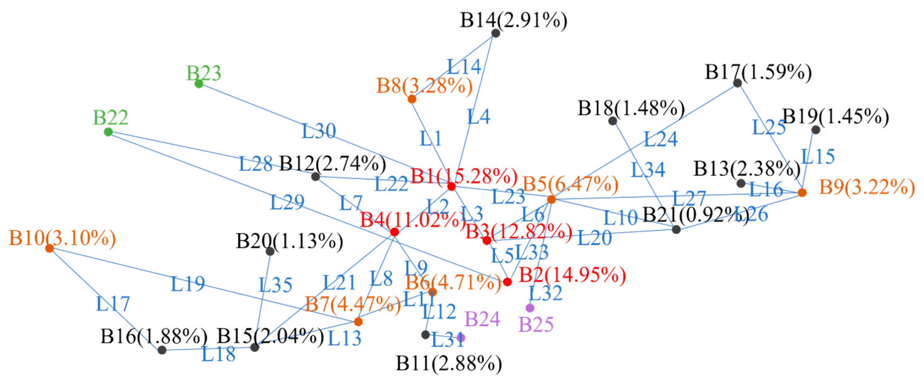
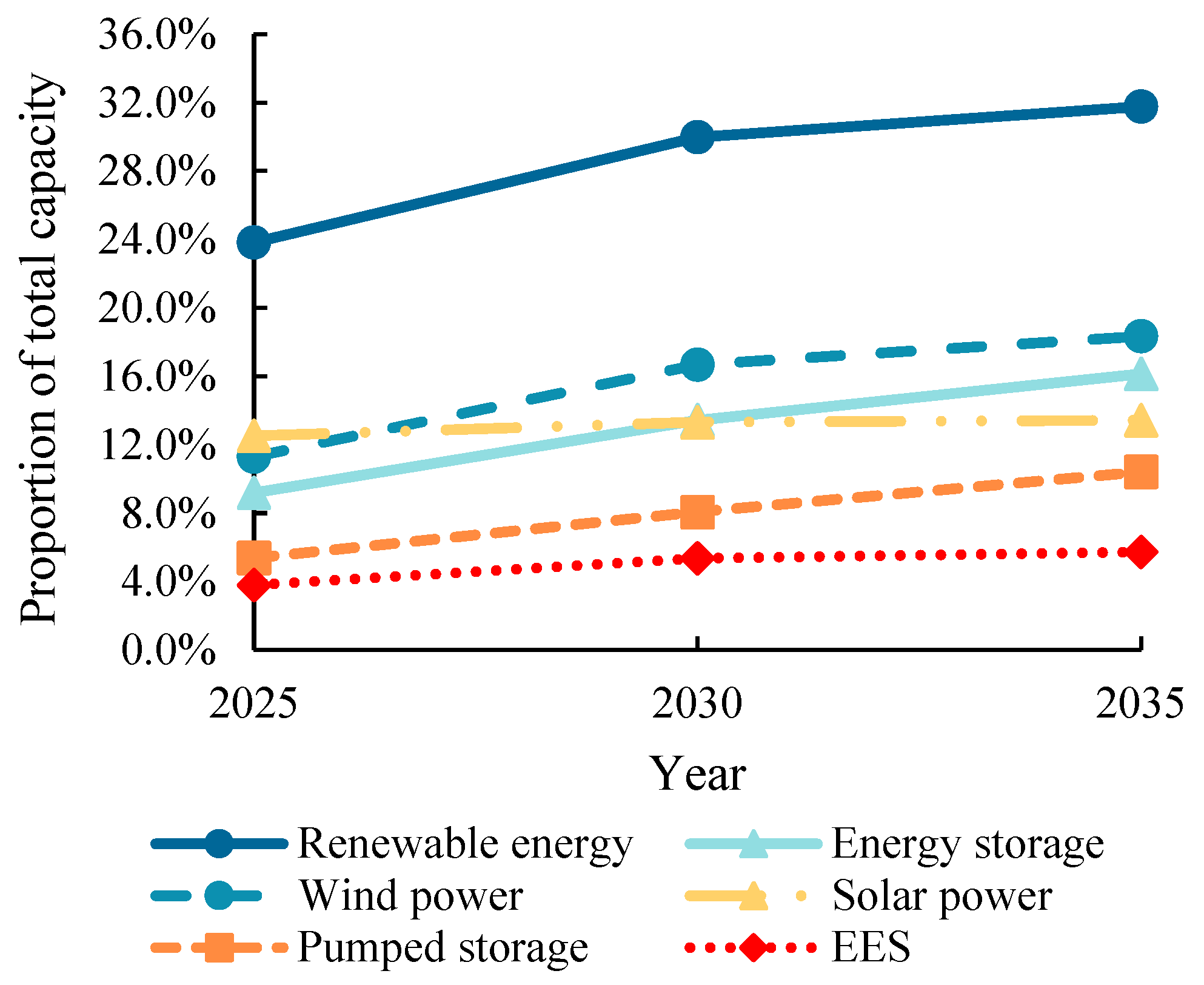
3.1. Power System Description and Scenario Classification Results

The impact of RE on transmission line load, as well as the effectiveness of the proposed rescheduling and energy storage planning method with a heavy load penalty function in reducing line heavy load rates and alleviating transmission congestion, was evaluated using a 25-bus system based on a modified power system from a province in China, as shown in Figure 2. The system under analysis represents a receiving-end power grid, with load concentrated in the central region. In this configuration, buses B22 and B23 serve as external power sources, while B24 and B25 function solely as load points, consuming power without supplying it back into the grid. B1 is assigned the highest load, with load values decreasing sequentially from B1 to B21. The highest demand for electricity in the entire power system was in August and the lowest was 66% of the former in February. The power system load in 2035 is 1.085 times that in 2030 and 1.254 times that in 2025.

According to the power source plan of the province for 2025, 2030, and 2035, multiple types of power supplies are available, including coal-fired power, gas-fired power, nuclear power, hydropower, wind power, solar power, EES, and pumped storage. From 2025 to 2035, the proportion of the total capacity of thermal power units decreased from over half at the beginning to approximately one-third, while the planned capacity and proportion in all power capacities of wind power, solar power, and energy storage gradually increased during these three stages, as shown in Figure 3. The EES involved in the system is mainly distributed in the load concentration area, whereas the pumped storage power stations are only partially distributed in the load concentration area, owing to the influence of geographical location. Moreover, this system is a receiving-end power network with a large and flexibly adjustable external power with a capacity of approximately 18% of the total capacity of the generators.

It should be mentioned that the research in this study is in a situation with unchanged transmission lines and changes in the power supply structure.

This simulation example considers the construction and maintenance costs of power sources as fixed values; therefore, these costs do not affect the scheduling optimization results and only the variable costs of each unit’s output are considered as the main economic factors for optimizing scheduling. The average cost per unit power of each type of generator is shown in

Table 2. Average cost per unit output of each type of power source for the power system.

Coal-Fired Power	Gas-Fired Power	Nuclear Power	Hydro-Power	Wind Power	Solar Power	EES	Pumped Storage	External Power
302	601	100	0	0	0	120	6	240

, whose RE includes its own free price, and the most expensive cost is from the gas power generator.

The predicted RE output was calculated using recent meteorological data, the planned capacity, and the RE output model. The meteorological data included wind speed at 100 m height and solar irradiance received per square meter obtained from the fifth-generation European Center for Medium-Range Weather Forecasts (ECMWF) [19]. For the relevant parameters in the model, the wind turbine parameters of a wind power commercial company were applied, as shown in

Table 3. Wind turbine parameters.

Model	Cut-In Speed (m/s)	Cut-Out Speed (m/s)	Rate Speed (m/s)	Rate Power (MW)	Application Scenario
MySE3.6-135	3	25	10.9	3.6	onshore
MySE6.45-18	3	30	10.5	6.45	offshore

[20]. A total of 50% of the wind power of areas near the sea, such as B11, B15, and B21, were calculated using the parameters of the offshore wind turbine MySE6.45-18.

Using the k-means clustering algorithm, three general scenarios are clustered, as shown in

Table 4. General scenario clustering results of days in 2025, 2030, and 2035.

Scenario	2025	2030	2035	Same
Scenario 1	108	96	115	82
Scenario 2	150	153	134	134
Scenario 3	107	116	116	99
Total	-	-	-	315

, and there is not much difference between the number of days of these scenes in the same year. The proportion of days with the same scenario in these three years was 86.3% of the entire year, whereas each general scenario had proportions of the same days from 71.3% to 100%. Because there are many same days of the same type of scenario in these three years, and it is appropriate for the study to be based on the data with the highest proportion of RE, scene classification results from 2035 are chosen as the general research scenario, which means that the same scenario in every year has the same days but their values are only related to the data of the specific year. When taking extreme scenarios into account, the average ratios of the net load to the load of each scenario in 2035 is illustrated in Figure 4. Scenario 4, with minimum net load, has a large RE electricity supply and small electricity demand, whereas Scenario 5, with the maximum net load, has the opposite performance.

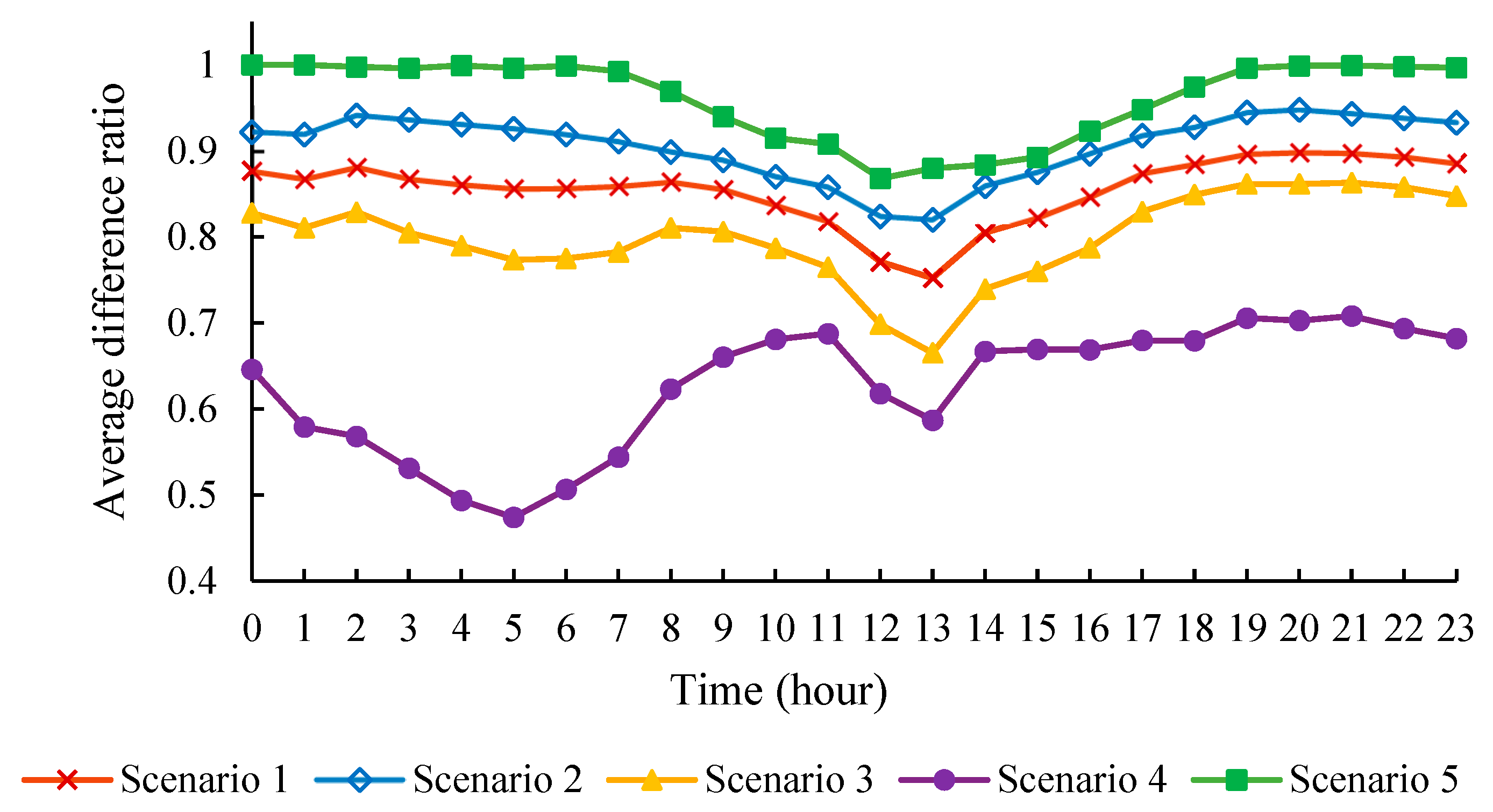
3.2. Result Analysis

The scheduling optimization model and energy storage planning model were developed using MATLAB 2021a and solved using the CPLEX 12.10 solver. In this section, the simulated and analyzed optimization objectives are $\mathrm{Objective}{’}_{\mathrm{operation}}$, minimizing the operating costs and RE waste.

The optimization results show that except for Scenario 4, which had an average RE abandonment rate of 0.96%, RE power outputs in other scenarios were fully utilized. From 2025 to 2035, the ALR, LRV, MLR, and ToHL (with LLR ≥ 0.8) of the five scenarios almost emerged in upward trends, as shown in

Table 5. Scheduling results for each scenario in 2025, 2030, and 2035.

	Scenario	Year	ALR	LRV	MLR	ToHL
General scenarios	Scenario 1	2025	0.233	0.002	0.932	9
		2030	0.260	0.006	1	11
		2035	0.272	0.009	1	47
	Scenario 2	2025	0.242	0.003	0.952	7
		2030	0.267	0.007	1	16
		2035	0.284	0.012	1	53
	Scenario 3	2025	0.207	0.003	0.941	3
		2030	0.228	0.008	0.899	12
		2035	0.254	0.010	1	51
Extreme scenarios	Scenario 4	2025	0.178	0.003	0.756	0
		2030	0.216	0.009	1	40
		2035	0.245	0.015	1	73
	Scenario 5	2025	0.230	0.003	0.889	7
		2030	0.236	0.006	0.902	13
		2035	0.260	0.012	1	46

. It is worth noting that Scenario 4, which had the largest proportion of RE electricity supply among these scenarios, grew in the LRV (from 0.003 to 0.015), MLR (from 0.756 to 1), and ToHL (from 0 to 73).

Although the system’s ALR is constantly increasing, a few lines do not keep pace with the overall trend. As for the LRV and MLR, almost all the lines have a common trend in growth from 2025 to 2035, even if the increased level of each line is developed differently. Taking Scenario 2 with the most clustering days as an example, it can be demonstrated in Figure 5, Figure 6 and Figure 7 that half of the lines have a higher ALR in 2035 compared to 2020 and 2025, while only one or two lines enhance the decreasing trend in the LRV and MLR in Scenario 2.

The contribution to the ToHL of the entire power system is mainly concentrated in lines L21, L23, L25, L26, and L29, as shown in Figure 8. Except for L25, almost all of these lines showed an obvious increase in the ToHL by 2035. There is a large amount of pumped storage whose ratio of capacity to load in B17, which is one end of the L25 connection, is improved from 0.79 in 2025 to 1.67 in 2035. Furthermore, some EES are arranged in B5, which is the other end of L25. Consequently, the line load of L25 is regulated by the energy storage, resulting in a decrease in the ToHL. Figure 9 illustrates the power of the pumped storage in B17, the power of the EES in B5, and the LLR of L25 in Scenario 2 of 2035.

In conclusion, the performance of the above indicators indicates that after more RE power plants are involved in the power system, the power fluctuation in the transmission line is more volatile, which means that lines are more prone to meet transmission congestion with a full load or heavy load, and most of the transmission lines maintain a heavy load status for a longer time without excessive help from the electricity storage system. On the other hand, the utilization rate roughly evaluated by the ALR may not necessarily improve with an increase in RE installation.

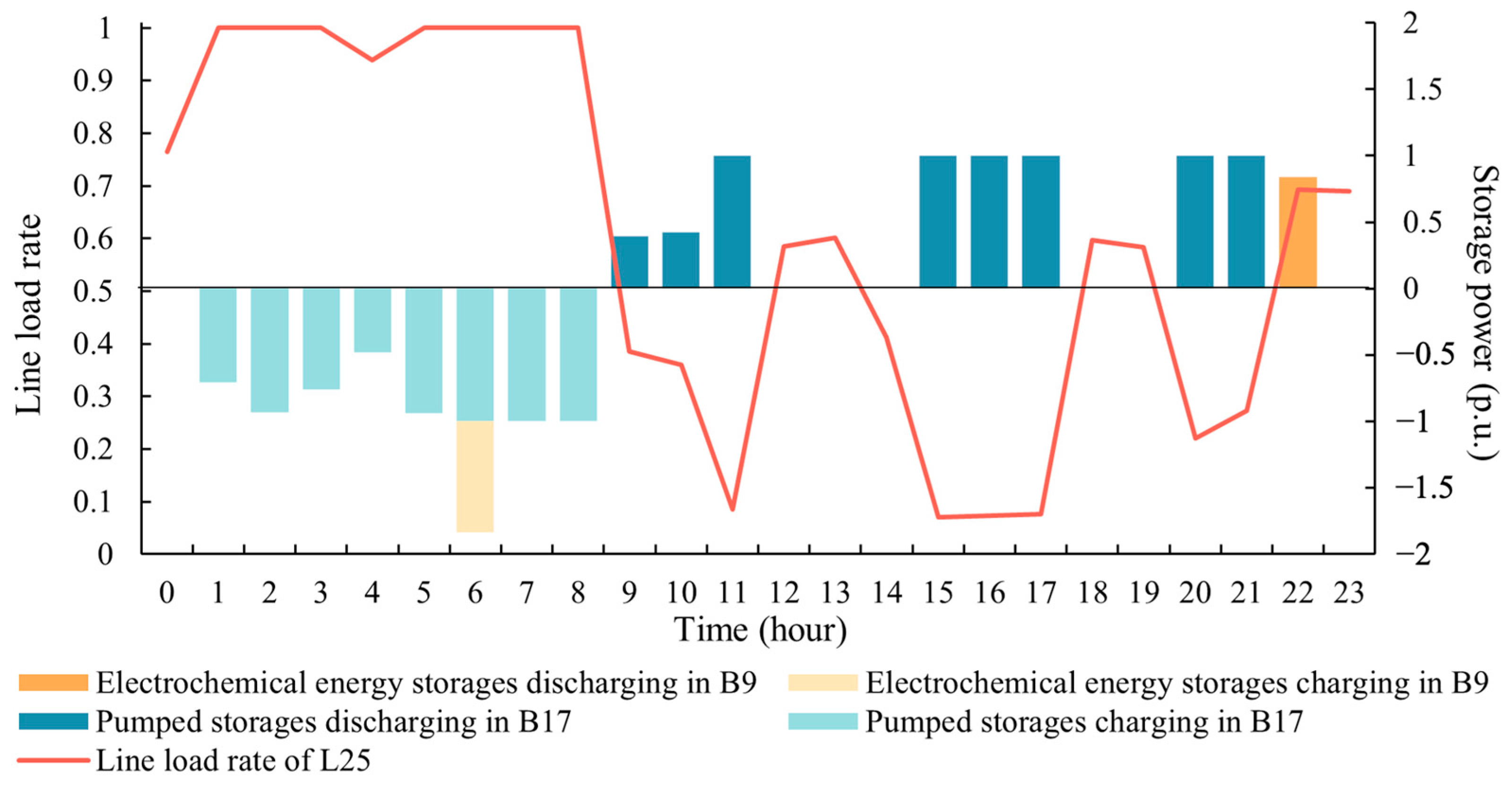
3.3. Results of Line Heavy Load-Alleviated Methods

There are two methods of rescheduling and planning to address the long-time heavy load problem of transmission lines by 2035.

The results of the newly planned energy storage by the planning model considering the heavy load of the lines are shown in

Table 6. Newly planned capacities of pumped storage and electrochemical energy storage.

	Bus Number	Capacity Proportion	Relational Lines
Pumped storage	1	4.4%	L1, L2, L3, L4, L22, L23, L30
	2	4.4%	L5, L29, L33
	3	4.4%	L3, L5, L6, L20
	6	8.8%	L9, L11, L12
	7	30.8%	L8, L11, L13, L19
	15	13.2%	L13, L18, L21, L35
	21	26.4%	L10, L20, L26, L34
EES	15	2.2%	L13, L18, L21, L35
	20	5.5%	L35

. Compared to EES, the planned pumped storage system has a larger storage capacity for long-term charging and discharging, which leads to more planning for pumped storage. Most of the lines with the heavy load problem obtain the planned energy storage at one of their ends, but there is no energy storage planned at any end of L25 because more energy storage is planned on B21, which is in the same grid section to alleviate the transmission pressure of L25.

Table 7. Results of line load indicators of different methods in each scenario in 2035.

Scenario	Method	ALR	LRV	MLR	ToHL
Scenario 1	Original	0.272	0.009	1	47
	Rescheduling	0.268	0.007	0.986	28
	Conventional plan	0.271	0.010	1	56
	Plan with heavy load	0.221	0.014	0.8	0
Scenario 2	Original	0.284	0.012	1	53
	Rescheduling	0.284	0.009	1	36
	Conventional plan	0.285	0.012	1	54
	Plan with heavy load	0.235	0.012	0.8	0
Scenario 3	Original	0.254	0.010	1	51
	Rescheduling	0.249	0.007	0.95	40
	Conventional plan	0.262	0.012	1	57
	Plan with heavy load	0.208	0.012	1	27
Scenario 4	Original	0.245	0.015	1	73
	Rescheduling	0.236	0.017	1	66
	Conventional plan	0.246	0.015	1	74
	Plan with heavy load	0.237	0.017	1	54
Scenario 5	Original	0.260	0.012	1	46
	Rescheduling	0.260	0.009	0.969	44
	Conventional plan	0.261	0.012	1	43
	Plan with heavy load	0.249	0.012	0.8	0

shows the line load indicator values of different schedules and plans in each 2035 scenario. The most effective method to reduce the time of heavy load for all lines is to plan energy storage considering line heavy load (plan with heavy load), followed by the rescheduling method. Although the fluctuation and utilization rate assessed by the LRV and ALR in the method of planning with a heavy load factor are worse than the original scheduling, they are in an acceptable range for a power system with more energy storage. In contrast, the rescheduling method balances these indicators while reducing the ToHL. Furthermore, the MLR of the plan with a heavy load is obviously smaller than the line capacity limit of 0.8 in Scenario 1, 2, and 5, which does not exceed the heavy load rate required by the power system. As for the two different planning methods, the increased energy storage does not help reduce the ToHL when only considering the line capacity limit.

The ToHL values of the main lines under heavy load conditions are listed in

Table 8. Time of heavy load for main lines by each method in all scenarios in 2035.

Scenario	Method	L2	L21	L23	L25	L26	L29
Scenario 1	Original	0	0	11	6	6	24
	Rescheduling	0	0	2	2	0	24
	Plan	0	1	12	7	12	24
	Plan with heavy load	0	0	0	0	0	0
Scenario 2	Original	0	4	14	8	3	24
	Rescheduling	0	2	4	4	2	24
	Plan	0	6	13	9	2	24
	Plan with heavy load	0	0	0	0	0	0
Scenario 3	Original	0	0	16	0	11	24
	Rescheduling	0	0	13	0	3	24
	Plan	0	0	19	0	14	24
	Plan with heavy load	2	24	0	1	0	0
Scenario 4	Original	1	24	11	0	20	17
	Rescheduling	0	24	11	0	20	11
	Plan	1	24	12	0	20	17
	Plan with heavy load	0	24	9	0	14	7
Scenario 5	Original	0	0	15	7	0	24
	Rescheduling	0	0	17	3	0	24
	Plan	0	0	13	6	0	24
	Plan with heavy load	0	0	0	0	0	0

. The ToHL of the plan with a heavy load was smaller than that of the other methods in most scenarios. The most significantly decreased line in this method is the external power transmission line L29, whereas L21 encounters a full load at all times in Scenario 3. However, it is still economical from an investment perspective when the expansion of L21 is adopted to address the subsequent problem of transmission congestion or heavy load rather than L29 because the length and unit cost of the external power transmission line L29, which transmits a large amount of electricity, is longer and more expensive than the provincial line L21. Figure 10 shows the LLR of L23 in Scenario 2 for each method. It can be seen that the LLR of L23 of the plan with a heavy load is obviously lower with a higher fluctuation than that of the other methods. Furthermore, the ToHL of the plan with heavy loads in Scenarios 1, 2, and 5, whose difference values between the load and RE output are smaller, is 0, which is also confirmed by the results of the MLR with 0.8, as shown in Table 7.

The performance of the rescheduling method on ToHL is slightly worse than that of the plan with a heavy load, mainly because of the outstanding contribution of reducing the ToHL of L29 in the latter method. The ToHL of almost all lines is the largest in the other planning methods without considering the heavy load penalty function.

In summary, the method of planning considering the heavy load penalty function effectively alleviates the heavy load on almost all lines compared with the original scheduling results. Using the rescheduling method to reduce the ToHL is also effective with a good balance of the load fluctuation and utilization rate of lines; however, the external power transmission line L29 with a large line load is still in a heavy load condition in this method. If a heavy load penalty is not involved in the planning model, the ToHL of the lines increases instead of decreases.

4. Conclusions

In this paper, we developed a scenario classification method based on the net load related with load and renewable energy (RE) output to study line load changes in future complex power systems. We constructed an optimization scheduling model incorporating multiple power sources to analyze line load under varying RE proportions. Methods for rescheduling and energy storage planning with a heavy load penalty function were proposed to mitigate heavy load times on transmission lines. Evaluation indices for line load, including the average load rate, load rate variance, maximum load rate, and heavy load time, were defined.

A case study on a Chinese provincial power system projected for 2025, 2030, and 2035 showed that increased RE proportions lead to higher line utilization rates, load fluctuations, maximum load, and heavy load times. Energy storage planning with a heavy load penalty function was found to be the most effective method to reduce heavy load time, followed by rescheduling with the penalty function.

The methods discussed, including scenario classification, load assessment indicators, and rescheduling and energy storage planning with overload penalty functions, are applicable for mitigating heavy loads on transmission lines in high-RE power systems. These approaches can provide an effective approach for the optimization of power system dispatch, helping the system to re-plan energy storage, enhance the system’s resilience in the face of the uncertainty issues of renewable energy, and improve the system’s adaptability to line load problems. Future analyses should consider a broader range of extreme weather scenarios impacting RE power systems and analyze the impact of extreme scenarios on TLHL system scheduling.

In future studies, extreme weather scenarios, such as prolonged low-wind conditions, heatwaves, or storms, can be considered to examine the model’s adaptability to sudden changes in RE availability.

References

1. Alomoush, M.I. Performance indices to measure and compare system utilization and congestion severity of different dispatch scenarios. Electr. Power Syst. Res. 2005, 74, 223–230. [Google Scholar] [CrossRef]
2. Yang, Q.; Wang, J.; Li, X.; Liu, H. A Bi-level transmission expansion planning model considering planning-operation coordination of line load rate indices. Power Syst. Technol. 2024, 48, 1846–1854. [Google Scholar]
3. Sun, W.; Wang, C.; Zeng, P.; Han, J. Review on evaluation method and index of power system homogeneity. Power Syst. Technol. 2015, 39, 1205–1212. [Google Scholar]
4. Yu, Q.; Cao, N.; Guo, J. Analysis on influence of load rate on power system self-organized criticality. Autom. Electr. Power Syst. 2012, 36, 24–27. [Google Scholar]
5. Dong, J.; Kong, L.; Li, C. Reduce the heavy overload rate of 10 kV distribution lines. Rur. Electr. 2021, 6, 50–53. [Google Scholar]
6. Koltsaklis, N.E.; Dagoumas, A.S. State-of-the-art generation expansion planning: A review. Appl. Energy 2018, 230, 563–589. [Google Scholar] [CrossRef]
7. Huang, H.; Li, Z.; Sampath, L.P.M.I.; Yang, J.; Nguyen, H.D.; Gooi, H.B.; Liang, R.; Gong, D. Blockchain-enabled carbon and energy trading for network-constrained coal mines with uncertainties. IEEE Trans. Sustain. Energy 2023, 14, 1634–1647. [Google Scholar] [CrossRef]
8. Yang, N.; Xiong, Z.; Ding, L.; Liu, Y.; Wu, L.; Liu, Z.; Shen, X.; Zhu, B.; Li, Z.; Huang, Y. A Game-Based Power System Planning Approach Considering Real Options and Coordination of All Types of Participants. Energy 2024, 312, 133400. [Google Scholar] [CrossRef]
9. Singh, V.; Fozdar, M.; Malik, H.; Márquez, F.P.G. Transmission congestion management through sensitivity-based rescheduling of generators using improved monarch butterfly optimization. Int. J. Electr. Power Energy Syst. 2023, 145, 108729. [Google Scholar] [CrossRef]
10. Li, Z.; Xu, Y.; Wang, P.; Xiao, G. Restoration of a Multi-Energy Distribution System with Joint District Network Reconfiguration via Distributed Stochastic Programming. IEEE Trans. Smart Grid 2024, 15, 2667–2680. [Google Scholar] [CrossRef]
11. Oree, V.; Hassen, S.Z.S.; Fleming, P.J. Generation expansion planning optimisation with renewable energy integration: A review. Renew. Sustain. Energy Rev. 2017, 69, 790–803. [Google Scholar] [CrossRef]
12. Mahdavi, M.; Antunez, C.S.; Ajalli, M.; Romero, R. Transmission Expansion Planning: Literature Review and Classification. IEEE Syst. J. 2019, 13, 3129–3140. [Google Scholar] [CrossRef]
13. Saboori, H.; Hemmati, R.; Ghiasi, S.M.S.; Dehghan, S. Energy storage planning in electric power distribution networks—A state-of-the-art review. Renew. Sustain. Energy Rev. 2017, 79, 1108–1121. [Google Scholar] [CrossRef]
14. Feng, C.; Shao, L.; Wang, J.; Zhang, Y.; Wen, F. Short-term Load Forecasting of Distribution Transformer Supply Zones Based on Federated Model-Agnostic Meta Learning. IEEE Trans. Power Syst. 2024, 1–13. [Google Scholar] [CrossRef]
15. Li, Z.; Wu, L.; Xu, Y.; Moazeni, S.; Tang, Z. Multi-stage real-time operation of a multi-energy microgrid with electrical and thermal energy storage assets: A data-driven MPC-ADP approach. IEEE Trans. Smart Grid 2021, 13, 213–226. [Google Scholar] [CrossRef]
16. Development and Reform Commission, Energy Bureau. Notice on Further Promoting the Participation of New Energy Storage in the Electricity Market and Dispatching Application (Operation of the Development and Reform Office [2022] No. 475). Beijing. Available online: https://zfxxgk.nea.gov.cn/2022-06/07/c_1310615910.htm (accessed on 1 October 2024).
17. Mansuwan, K.; Jirapong, P.; Thararak, P. Optimal battery energy storage planning and control strategy for grid modernization using improved genetic algorithm. Energy Rep. 2022, 9, 236–241. [Google Scholar] [CrossRef]
18. Yu, H.; Ye, C.; Ding, Y.; Song, Y. Power System Optimal Dispatch Integrating the Responsive High-Speed Train Fleet. IEEE Trans. Smart Grid 2024. [Google Scholar] [CrossRef]
19. Chen, J.; Hu, H.; Wang, M.; Ge, Y.; Wang, K.; Huang, Y.; Yang, K.; He, Z.; Xu, Z.; Li, Y.R. Power Flow Control-Based Regenerative Braking Energy Utilization in AC Electrified Railways: Review and Future Trends. IEEE Trans. Intell. Transp. Syst. 2024, 25, 6345–6365. [Google Scholar] [CrossRef]
20. Yao, L.; Zhang, Q.; Wu, J.; Saniye, M. Study on MES optimal probability power flow considering source and load uncertainties. Pow. Capacit. React. Pow. Compens. 2022, 47, 57–66. [Google Scholar]
Figure 1. The steps of k-means clustering.
Processes 12 02725 g001
Figure 2. The proportion of power load at each bus of the 25-bus system.
Processes 12 02725 g002
Figure 3. Proportion of RE and ESP capacity.
Processes 12 02725 g003
Figure 4. The average ratio of the net load to the load in each scenario in 2035.
Processes 12 02725 g004
Figure 5. Average load rate of all lines for three stages in Scenario 2.
Processes 12 02725 g005
Figure 6. Load rate variance of all lines for three stages in Scenario 2.
Processes 12 02725 g006
Figure 7. Maximum load rate of all lines for three stages in Scenario 2.
Processes 12 02725 g007
Figure 8. Time of heavy load for main lines having values of heavy load in each scenario and year.
Processes 12 02725 g008
Figure 9. The generation of energy storage at each end of L25 and its line load rate in Scenario 2 in 2035.
Processes 12 02725 g009
Figure 10. Line load rate of L23 of each method in Scenario 2 in 2035.
Processes 12 02725 g010