Kick Risk Diagnosis Method Based on Ensemble Learning Models

Abstract

As oil and gas exploration and development gradually advance into deeper and offshore fields, the geological environment and formation pressure conditions become increasingly complex, leading to a higher risk of drilling incidents such as kicks. Timely diagnosis of kick risk is crucial for ensuring safety and efficiency. This study proposes a kick risk diagnosis method based on ensemble learning models, which integrates various time-series analysis algorithms to construct and optimize multiple kick diagnosis models, accurately fitting the relationship between integrated logging parameters and kick events. By incorporating high-performance ensemble models such as Stacking and Bagging, the accuracy and F1 score of the models were significantly improved. Furthermore, the application of the Synthetic Minority Over-sampling Technique and Tomek Links (SMOTE-Tomek) data balancing technique effectively addressed the issue of data imbalance, contributing to a more robust and balanced model performance. The results demonstrate that integrating time-series analysis with ensemble learning methods significantly enhances the predictive reliability and stability of kick monitoring models. This approach provides a dependable solution for addressing complex kick monitoring tasks in offshore and deepwater drilling operations, ensuring greater safety and efficiency. The findings offer valuable insights that can guide future research and practical implementation in kick risk diagnosis.

1. Introduction

Currently, oil and gas exploration and development are increasingly expanding into complex areas such as deep, ultra-deep, unconventional, low-permeability, mature fields, and deepwater offshore environments. In particular, ultra-deep drilling poses significant challenges due to numerous unknown factors, high-temperature and high-pressure formations, hard and abrasive rock, among other difficulties [1]. These factors increase the risks and complexities associated with well construction, leading to a higher likelihood of incidents such as kick or blowouts. Improper handling of kick incidents may escalate to complex situations like blowouts, resulting in well abandonment, threats to the safety of personnel, and substantial economic losses. At present, kick diagnosis methods can be broadly categorized into conventional and intelligent diagnostic methods. Traditional kick diagnostic approaches face challenges in terms of timeliness and accuracy, while intelligent diagnostic methods, despite their promising prospects, still face limitations in generalization capability and have limited practical applications in the field. This situation highlights the urgent need for in-depth research on intelligent diagnostic methods for kick detection in drilling operations.

Orban et al. [2] proposed a small error flowmeter, which not only offers high measurement accuracy but is also applicable for measuring the flow rate of both water-based and oil-based muds. Schafer et al. [3] introduced a development-type rolling float flowmeter designed to accurately measure the outflow of pipeline fluids, demonstrating excellent measurement performance. Peter Ablard et al. [4] utilized a Coriolis flowmeter capable of operating at low to medium pressure, eliminating the impact of temperature and accurately measuring the mass flow rate, temperature changes, and density of oil, gas, and water in the pipeline. Helio Mauricio Santos et al. [5] developed a microflow kick monitoring technology that employs sonar detectors, achieving significant results in kick monitoring. Deng Yong et al. [6] employed sonar detectors to monitor liquid level changes in the wellhead conductor and separator, achieving flow monitoring during both well-opening and well-shutdown periods for early warning of kicks.

Hargreaves et al. [7] monitored deepwater drilling kicks using a Bayesian probability method. By analyzing acoustic data, they employed a Bayesian model to calculate the probability of a kick occurring, thereby determining the likelihood of a kick event. Additionally, Yue et al. [8] developed a novel early warning system for kicks by combining hierarchical Bayesian methods with expert systems. Gurina et al. [9] constructed a classification model based on gradient-boosted decision trees, using Measurement While Drilling (MWD) data to predict drilling kick risks. However, although this algorithm can identify about half of the anomalies, it generates approximately 53% false alarms on average each day. Lian [10] proposed a fusion algorithm using rough set support vector machines to monitor drilling incidents. Nhat et al. [11] proposed a data-driven Bayesian network model for early kick detection using data obtained from laboratory experiments, leveraging downhole parameters. Kamyab et al. [12] employed a focused time-delay dynamic neural network for real-time monitoring of early kicks, calculating dynamic drilling parameters in real time through a neural network to monitor kick conditions. Lind et al. [13] utilized k-means clustering and radial basis function neural network models to predict drilling risks for oil and gas wells. Zhang et al. [14] summarized the characterization parameters and patterns of kicks, establishing an intelligent early warning model based on BP neural networks, which demonstrated high accuracy and timeliness in its warning results. Duan et al. [15] proposed the identification of kick risk based on the identification of drilling conditions. Zhu et al. [16] conducted kick risk monitoring using an unsupervised time-series intelligent model, achieving an accuracy of 95%. Single time-series intelligent models, such as LSTM and GRU, are capable of capturing nonlinear features and long-term dependencies in time-series data, but they also have significant drawbacks. Firstly, they are prone to overfitting, especially when the data are limited or noisy, which results in poor generalization ability. Secondly, these models are susceptible to local minima, leading to unstable training and difficulty in capturing complex patterns in the data. Additionally, single models have limited robustness, with poor adaptability to outliers and data fluctuations, and their prediction results can be significantly affected by the quality of the data. While single time-series intelligent models can capture nonlinear features and long-term dependencies, they also have clear limitations. Ensemble time-series models, by combining multiple different models, can address these shortcomings of single time-series models.

In the early stages of kick events, the comprehensive logging data often exhibit complex inter-related changes and nonlinear fluctuations in time series. These features not only reflect the interactions of multiple factors but also demonstrate the intricate relationships between time and space. However, current intelligent diagnostic methods generally utilize non-temporal single-point data as training sets for modeling, which fail to adequately capture the dynamic temporal attributes of kick events. The lack of effective utilization of time-series information results in difficulties in deeply analyzing the intrinsic connections of multidimensional data across spatial and temporal dimensions. Consequently, the models become overly sensitive to the original structure of the data and fail to effectively leverage spatiotemporal information, thereby limiting improvements in the accuracy of kick risk diagnosis. To address this issue, time-series models based on ensemble learning can significantly enhance model accuracy by integrating multiple algorithms and models to comprehensively consider the trends and dynamic features of time-series data. This approach enables the extraction of latent information from time-series data, identifying key features at different time points and spatial locations, which aids in a more comprehensive understanding of the mechanisms behind kick events. Furthermore, the introduction of the Synthetic Minority Over-sampling Technique and Tomek Links (SMOTE-Tomek) data balancing technique can effectively address the imbalance problem within the dataset, enhancing the model’s ability to identify minority class samples (kick events). SMOTE-Tomek improves the model’s generalization capability by increasing the number of minority class samples and reducing noise samples, making it more reliable in practical applications. Therefore, employing a time-series model based on ensemble learning, combined with the SMOTE-Tomek technique, will help improve the accuracy and reliability of kick risk diagnosis.

2. Methodology

2.1. SMOTE-Tomek Algorithm

SMOTE-Tomek is a data balancing method that combines SMOTE and Tomek Links, specifically designed to address the issue of imbalanced classification. First, SMOTE increases the number of minority class samples by generating new synthetic samples between existing minority class instances, thus enhancing the proportion of the minority class in the dataset and preventing the model from being biased towards the majority class during training [17]. Next, Tomek Links identifies and removes pairs of samples that are close to the boundary between different classes, particularly those that can lead to classification confusion [18]. By deleting the majority class samples in these pairs, Tomek Links reduces the presence of hard-to-distinguish samples in the dataset, thereby optimizing the classification boundaries.

For the kick sample data, which presents a highly imbalanced classification problem, the application of SMOTE-Tomek can effectively increase the number of kick class (minority class) samples while cleaning up noise and boundary samples in the data.

2.2. The Long Short-Term Memory (LSTM)

The Long Short-Term Memory (LSTM) network is a specialized branch of recurrent neural networks (RNNs) designed to overcome the vanishing gradient problem encountered by traditional RNNs when handling long-distance sequence dependencies [19]. By incorporating a gating mechanism, LSTM effectively retains and transmits critical information, demonstrating exceptional ability in learning long-term temporal dependencies. The structure of an LSTM unit consists of three main gates: the forget gate, which decides what information should be discarded from the cell state; the input gate, which determines what new information should be added to the cell state; and the output gate, which decides what information should be output from the current cell state. This gating mechanism allows LSTM to selectively retain or ignore information, ensuring that relevant data are kept while irrelevant information is discarded, thereby supporting precise learning and prediction in scenarios with long-term dependencies. Due to this unique advantage, LSTM is widely applied in various contexts requiring an in-depth analysis of temporal relationships in input data, such as time-series anomaly detection. The LSTM network structure is shown in Figure 1.

2.3. The Gated Recurrent Unit (GRU)

The Gated Recurrent Unit (GRU) is another variant of the recurrent neural network (RNN), designed to address the issues of long-term dependencies and vanishing gradients in traditional RNNs [20]. Compared to the RNN, GRU introduces the concepts of an update gate and a reset gate to control the flow and retention of information. The reset gate determines whether to ignore the information from the previous hidden state at the current time step, while the update gate decides how to combine the input at the current time step with the previous hidden state to generate a new hidden state. This gating mechanism allows GRU to more effectively remember and update information when processing long sequences, making it well-suited for various sequence modeling tasks. The GRU network structure is shown in Figure 2.

In comparison, GRU simplifies the design of LSTM by merging the forget gate and input gate into a single update gate and removing the cell state, retaining only the hidden state. This simplification not only reduces the number of parameters in the model, improving computational efficiency, but also maintains performance levels comparable to LSTM in many cases. Particularly in tasks with relatively small datasets or those requiring fast model training, GRU’s simplified architecture is easier to optimize. Given the challenges of collecting kick data and the limited availability of effective samples, GRU’s simpler structure is more suited to the needs of kick detection. Additionally, real-time kick diagnosis requires the model to operate quickly to meet real-time standards, making GRU’s advantages in speed especially significant.

2.4. Temporal Autoencoder

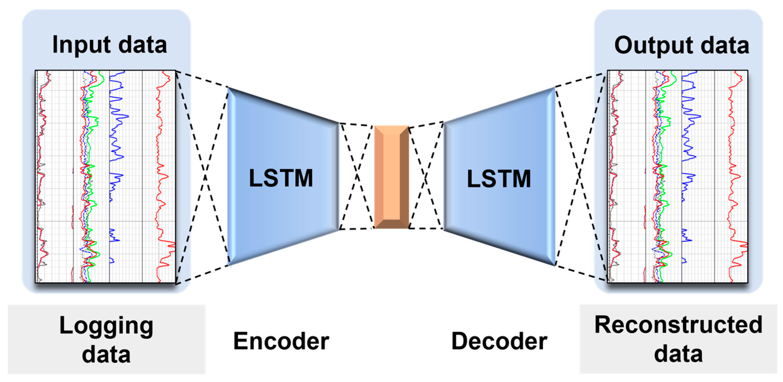
The temporal autoencoder is a neural network model designed to handle data with temporal structures. Similarly to traditional autoencoders, a temporal autoencoder consists of two parts—an encoder and a decoder—with the main objective of learning a compact representation of the data and being able to reconstruct the input. However, unlike ordinary autoencoders, temporal autoencoders take time dimension information into account when processing temporal data. Specifically, the encoder and decoder not only learn the spatial features of the data but also capture the temporal evolution patterns [21].

In a temporal autoencoder, the encoder first maps the input sequence to a lower-dimensional representation, commonly referred to as the encoding or hidden state. This hidden state contains the key information of the input sequence, including its temporal evolution. The decoder then decodes this hidden state into an output sequence of the same dimensionality as the original input sequence to reconstruct the original data. During training, the temporal autoencoder learns to minimize the reconstruction error, enabling the encoder to capture important features in the data while preserving the structure of the time series. The temporal autoencoder structure is shown in Figure 3.

Temporal autoencoders have been widely applied in the modeling and analysis of time-series data, especially showing significant advantages in handling anomaly detection tasks. Given the scarcity of kick data samples and the abundance of normal, non-kick data, temporal autoencoders can effectively identify anomalous behaviors by learning the intrinsic representation of normal data and detecting patterns that deviate from the normal mode, thereby facilitating kick detection. This mechanism is particularly useful in imbalanced data scenarios, where it can still accurately identify abnormal patterns, providing a reliable technical means for the timely detection and prevention of kicks.

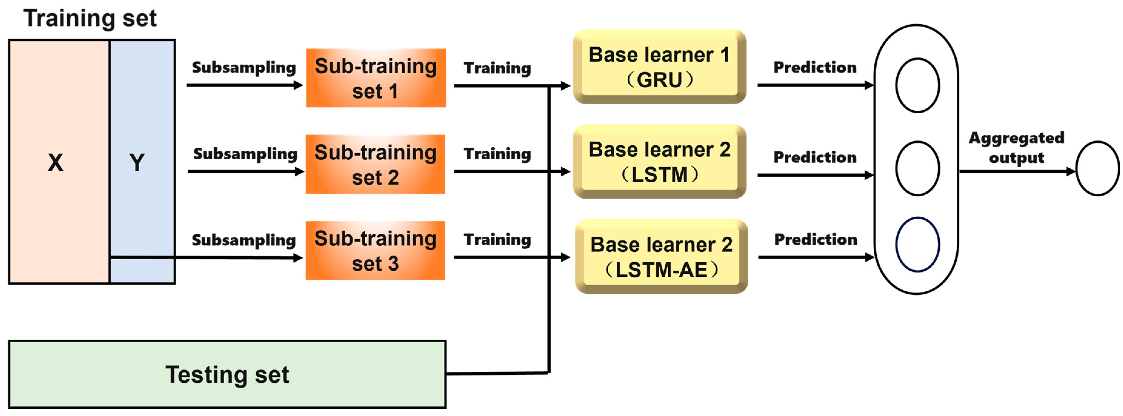
2.5. Ensemble Learning

Ensemble learning improves classification performance by building and combining multiple models. The core idea of this approach is to combine several weak learners to form a strong learner, thereby enhancing the model’s generalization ability. Ensemble learning primarily reduces variance by training multiple models in parallel and averaging their classification results or using majority voting, or it reduces bias by sequentially training multiple models, with each model attempting to correct the errors of the previous one. Ensemble learning has demonstrated superior performance in many practical applications. Bagging, Random Forest, Stacking, and Boosting are common types of ensemble learning methods. The ensemble learning structure is shown in Figure 4.

Bagging (Bootstrap Aggregating) involves repeatedly sampling the original dataset with replacements to create multiple training sets, which are then used to train several models [22]. The classification results of these models are aggregated through voting or averaging to form a final decision. This method helps reduce the variance of the model, improving its stability and accuracy, and is particularly suitable for addressing overfitting issues. Random Forest, an extension of Bagging, constructs a strong classifier by training multiple decision trees using random samples and random feature subsets. By introducing randomness in both data sampling and feature selection, Random Forest effectively reduces the variance seen in a single decision tree, resulting in a more stable model. This approach ensures that the combined model performs well across different datasets by mitigating overfitting.

Stacking is a method that integrates the classification abilities of various base models [23]. Its core strategy involves using a new model, called a meta-learner, to optimally combine the classification results of these base models. In this approach, each base model is first trained on the original dataset to produce classification results, which are then treated as a new dataset for training the meta-learner. By doing so, the Stacking method aims to capture complementary information among different models, significantly enhancing classification accuracy.

Boosting is a technique designed to reduce bias by sequentially training models, where each model aims to correct the errors of its predecessor. This iterative approach ensures that each subsequent model becomes progressively better at classifying hard-to-predict samples, effectively minimizing bias over time. Popular Boosting algorithms, such as AdaBoost and Gradient Boosting, increase the weights of misclassified samples in each iteration, making the final ensemble highly accurate. This step-by-step correction enhances the model’s overall performance, especially for complex datasets.

Ensemble learning significantly enhances model accuracy by merging the classification results of multiple models, allowing it to identify patterns that a single model may overlook when dealing with complex problems. Compared to the overfitting issues common in single models, ensemble methods reduce the risk of overfitting and improve generalization ability by introducing randomness and regularization. Additionally, combining multiple models effectively lowers prediction variance and increases the stability of classification results. Therefore, to improve the accuracy and reliability of kick diagnosis models, adopting an ensemble learning strategy is an effective approach.

3. Data Processing

3.1. Data Source

In this study, we collected and organized comprehensive logging time-series data from over 130 wells. These wells experienced more than 140 kick events during drilling operations. The dataset underwent strict selection and quality control processes, excluding corrupted files and records with missing key parameters such as inlet and outlet flow rates and total pit volume. After completing this initial screening, we performed extensive data preprocessing and analysis on the high-quality kick case data files. Ultimately, comprehensive logging time-series data from 76 wells and 80 kick events were selected for further study.

3.2. Feature Selection

To improve the predictive accuracy of the model, reduce the risk of overfitting, decrease training time, enhance model interpretability, and reduce the costs of data collection and storage, feature selection is necessary. By carefully choosing the most influential features, it is possible to simplify the model’s complexity and enhance operational efficiency while maintaining performance, which is crucial for building efficient and reliable data-driven decision models. In feature selection, the Spearman correlation coefficient is used to analyze the correlation between features. Spearman’s coefficient is a statistical measure that quantifies the strength of the linear relationship between two variables, with values ranging from −1 to 1. Specifically, a value of 1 indicates a perfect positive correlation between two variables, while a value of −1 indicates a perfect negative correlation; a value of 0 indicates no correlation between the variables. By evaluating the Spearman correlation coefficients between features and between features and the target variable, it is possible to effectively identify features that have a significant impact on the prediction target, while excluding redundant or low-correlation features, thereby optimizing the feature set and improving the model’s performance and interpretability [24]. The Spearman calculation formula is shown in Equation (1).

$$r_s=1-{\displaystyle \frac{6{\displaystyle \sum _{i=1}^n{d}_i^2}}{n\left(n^2-1\right)}}$$

(1)

where $r_s$ represents the final Spearman correlation coefficient value between the two variables, $n$ is the number of data points in the variables, and $d_i^2$ is the squared difference in ranks between the sorted data of the two variables.

The correlation coefficients between features and kick are shown in Figure 5. After analyzing the comprehensive field knowledge, expert experience, and various feature selection methods mentioned above, this study ultimately selected the following seven parameters as input features for building the intelligent model: outlet flow rate, Standpipe Pressure, total pit volume, Weight on Bit, Hook Load, Outlet Density, and Torque. Among these, the correlation coefficients of outlet flow rate, Standpipe Pressure, and total pit volume with the kick label ranked among the top. This result aligns well with practical engineering field observations and expert experience.

3.3. Smoothing Filter

In this study, the Savitzky–Golay filter was applied to process the data, and its effects on the trends were analyzed. The Savitzky–Golay filter is a data smoothing technique based on local polynomial regression, where a polynomial function is fitted to a set of neighboring data points to approximate their distribution. The essence of this method lies in its ability to preserve important features, such as peaks and valleys, while smoothing out high-frequency noise. The filter works by replacing each data point with the value predicted by the fitted polynomial, ensuring that the underlying data trends are preserved. The basic formula of the Savitzky–Golay method, shown in Equation (2), expresses the smoothed value of a data point as a weighted sum of the neighboring values, where the weights are determined by the coefficients of the polynomial fit. These coefficients are computed using a least-squares fitting approach, which ensures the best approximation of the data within a specified window. This approach allows the smoothing process to be flexible, as the window size and polynomial degree can be adjusted to optimize the results for different data characteristics. By applying this technique, the study was able to reduce noise and maintain the overall data trends, facilitating clearer analysis and interpretation. The comparison before and after applying the Savitzky–Golay filter is shown in Figure 6.

$$y_i^{\prime }={\displaystyle \frac{1}{n}}{\displaystyle \sum }_{j=-m}^m{c}_j\cdot y_{i+j}$$

(2)

where $y_i^{\prime }$ represents the filtered value, $y_{i+j}$ is the value at the ($i+j$)th point in the original sequence. $c_j$ represents the polynomial coefficients, which depend on the window size and the degree of the polynomial. $n$ is the normalization factor for the coefficients, typically denoted as $n={\displaystyle \sum }_{j=-m}^m{c}_j$. m is the width of one side of the window, and the total window size is 2m + 1.

3.4. Non-Dimensionalization

In the process of intelligent modeling, transforming variables with physical units into unit-free forms is a critical step aimed at eliminating the influence of dimensionality, scale, and distribution on model performance. By normalizing data to a unified range, the model’s generalization ability can be enhanced, allowing it to adapt to different scales and conditions and avoid dependency on specific unit systems, thus simplifying the complexity of problem-solving. Two commonly used methods for non-dimensionalization are standardization and normalization. Standardization is a process that transforms data into a distribution centered at zero (mean equals zero) with a unit standard deviation (standard deviation equals one). This method is particularly useful for analytical scenarios that assume the data follow a standard normal distribution. The calculation formula is shown in Equation (3).

$$z={\displaystyle \frac{\left(x-\mu \right)}{\sigma }}$$

(3)

where x represents the original data point, μ is the mean of the entire dataset, σ is the standard deviation of the entire dataset, and z is the standardized data point.

4. Model Establishment

4.1. Evaluation Metrics for Intelligent Classification Models

This study focuses on the issue of kick diagnosis, which is essentially a binary classification problem. To comprehensively evaluate the performance of the adopted models, this paper not only employs standard metrics used in classification evaluations, such as accuracy, precision, and recall, but also introduces missing alarm rate (MAR) and false alarm rate (FAR) as evaluation tools. Additionally, to balance precision and recall, as well as MAR and FAR, the F1 score is used to analyze and assess the model’s performance. These metrics are calculated using a confusion matrix, also known as a contingency matrix or error matrix, which is a table that provides a detailed overview of the model’s classification results, as shown in

Table 1. Confusion matrix.

True Result	Forecast Result
	Positive Class	Negative Class
Positive class	TP	FN
Negative class	FP	TN

. However, to further assess the model’s performance across different classification thresholds, the Area Under the Curve (AUC) of the Receiver Operating Characteristic (ROC) curve was also included.

The accuracy formula is given by Equation (4).

$$Accuracy={\displaystyle \frac{TP+TN}{TP+FN+TN+FP}}$$

(4)

The recall formula is given by Equation (5).

$$Recall={\displaystyle \frac{TP}{TP+FN}}$$

(5)

The precision formula is given by Equation (6).

$$Precision={\displaystyle \frac{TP}{TP+FP}}$$

(6)

The missing alarm rate formula is given by Equation (7).

$$MissingAlarmRate={\displaystyle \frac{FN}{TP+FN}}$$

(7)

The false alarm rate formula is given by Equation (8).

$$FalseAlarmRate={\displaystyle \frac{FP}{TP+FP}}$$

(8)

The F1 score formula is given by Equation (9).

$$F1score=2\cdot {\displaystyle \frac{Precision\times Recall}{Precision+Recall}}$$

(9)

4.2. Model Implementation and Optimization

In this study, we developed the LSTM, GRU, LSTM Autoencoder (LSTM-AE) models, as well as intelligent models based on Bagging and Stacking ensemble strategies.

4.2.1. LSTM and GRU

We developed LSTM- and GRU-based kick intelligent diagnosis models using the Python language. In classification problems, common loss functions include cross-entropy loss, mean squared error loss, exponential loss, and logarithmic loss. Each of these functions is suitable for different scenarios and requirements. For the binary classification problem in this study, the binary cross-entropy loss function is the most appropriate choice, as it directly quantifies the difference between the actual output and the predicted output. The formula is shown in Equation (10).

$$L\left(y,p\right)=-\left[y\log \left(p\right)+\left(1-y\right)\log \left(1-p\right)\right]$$

(10)

where $L\left(y,p\right)$ represents the value of the loss function; y is the true label, taking the value 0 or 1, where 0 indicates non-kick and 1 indicates a kick; p is the probability predicted by the model that a sample belongs to a kick; $\log \left(p\right)$ and $\log \left(1-p\right)$ represent the natural logarithms of the predicted probability and its complement, respectively.

To optimize the hyperparameters of the LSTM and GRU models effectively, we used an advanced hyperparameter optimization tool in Python called the Optuna library. Optuna can automatically search for the best hyperparameter combinations using Python’s conditional statements and loop structures. This library accelerates the process of obtaining results by efficiently exploring large hyperparameter spaces and discarding unpromising trials. Additionally, Optuna supports easy parallelization of hyperparameter searches across multiple threads or processes without requiring any changes to the code. When Optuna is used for optimizing intelligent algorithms, the objective function typically returns the model’s loss or accuracy. In this study, for kick diagnosis, we aim to achieve relatively low levels of both the missing alarm rate and the false alarm rate. LSTM and GRU parameter optimization is shown in

Table 2. LSTM and GRU parameter optimization.

Model	Parameter	Parameter Range	Optimal Value	Parameter Description
LSTM	lstm_units1	32, 64, 128, 256	32	Number of Neurons in the First LSTM Layer
	lstm_units2	8, 16, 32, 64, 128	16	Number of Neurons in the Second LSTM Layer
	learning_rate	0.0001, 0.001, 0.01	0.001	Learning Rate of the Optimizer
	dropout_rate	0.2, 0.3, 0.4	0.3	Dropout Rate to Prevent Overfitting
	epochs	100, 200, 300, 400, 500	300	Number of Training Epochs
	batch_size	32, 64, 128	64	Number of Samples per Training Iteration
GRU	gru_units1	32, 64, 128, 256	64	Number of Neurons in the First GRU Layer
	gru_units2	8, 16, 32, 64, 128	32	Number of Neurons in the Second GRU Layer
	learning_rate	0.0001, 0.001, 0.01	0.01	Learning Rate of the Optimizer
	dropout_rate	0.2, 0.3, 0.4	0.2	Dropout Rate to Prevent Overfitting
	epochs	100, 200, 300, 400, 500	500	Number of Training Epochs
	batch_size	32, 64, 128	64	Number of Samples per Training Iteration

.

The selection of these parameter ranges is based on commonly used values in deep learning research and practice, aiming to balance model complexity and performance. For the number of units in LSTM and GRU layers, the chosen range (32, 64, 128, 256) covers different requirements from simple to complex model structures, ensuring the model can adapt to various levels of data complexity. The learning rate range (0.0001, 0.001, 0.01) is drawn from typical values in optimization algorithms to balance training speed and convergence stability. The dropout rate range (0.2, 0.3, 0.4) is selected to strike a balance between preventing overfitting and maintaining the model’s learning capacity. The range of training epochs (100 to 500) allows sufficient time for effective training without overfitting, while the batch size range (32, 64, 128) is chosen to balance training time and gradient update stability. These reasonable parameter ranges enable comprehensive exploration and optimization of the model under various conditions to achieve optimal performance.

Hyperparameter tuning is conducted using methods such as cross-validation or grid search to explore the impact of different parameter combinations on model performance. In this study, these parameter ranges were chosen to ensure comprehensive coverage of potential optimal configurations within reasonable computational resources. During the tuning process, the model’s performance on the validation set was used as a basis for selecting the optimal parameters. The optimal values (as shown in the table) were typically chosen when the model achieved stable and high performance, ensuring maximum effectiveness on both training and testing data.

4.2.2. LSTM-AE

This study selected the LSTM-AE model, with both its encoder and decoder being LSTM networks. This model learns a compressed representation of the input data to reconstruct the output data, thereby capturing the temporal dependencies and patterns in time-series data. This structure is particularly suitable for tasks such as time-series analysis, anomaly detection, and feature extraction, making it highly applicable to the drilling risk kick monitoring problem addressed in this study. LSTM-AE parameter optimization is shown in

Table 3. LSTM-AE parameter optimization.

Model	Parameter	Parameter Range	Optimal Value	Parameter Description
LSTM-AE	batch	32, 64, 128	32	Batch Size
	encoder_lstm_units1	8, 16, 32, 64	32	Number of Neurons in the First Encoder Layer
	encoder_lstm_units2	2, 4, 8	4	Number of Neurons in the Second Encoder Layer
	repeat_vector_num	4, 8, 16	8	Number of Repeat Vector Times
	decoder_lstm_ units1	2, 4, 8	8	Number of Neurons in the First Decoder Layer
	decoder_lstm_ units2	8, 16, 32, 64	16	Number of Neurons in the Second Decoder Layer
	Threshold_train	0.1, 1, 10	0.1	Reconstruction Error Threshold for the Training Set
	Threshold_val	50–250	185	Reconstruction Error Threshold for the Validation Set

.

4.2.3. Bagging-Based Ensemble Strategy

The flowchart of the Bagging ensemble learning strategy is shown in Figure 7. When implementing the Bagging ensemble learning strategy to build the model, data samples are repeatedly drawn with replacement to generate three training data subsets. Due to the nature of sampling with replacement, each subset may contain duplicate samples and may omit some original samples. These subsets are then used to independently train the base learners GRU, LSTM, and LSTM-AE. Since the LSTM-AE network belongs to the unsupervised learning category, its training differs from the other models, relying only on non-kick samples from the training data subset. Finally, the results from the three models are combined using the majority voting method to obtain the final classification result. In the Bagging ensemble method, no additional hyperparameters are introduced. The method primarily relies on the inherent hyperparameters of each base learner, with the optimization process focused on enhancing model performance by optimizing these existing hyperparameters.

4.2.4. Stacking-Based Ensemble Strategy

The flowchart of the Stacking ensemble learning strategy is shown in Figure 8. The GRU and LSTM base models are trained using a labeled dataset, while the LSTM-AE base model is trained using an unlabeled dataset to ensure diversity among the algorithms. All these base learners are trained on the complete training dataset and produce corresponding classification results, which serve as inputs for the next step. Then, the classification results from these base learners are treated as new features, called meta-features, and combined with the original feature set to form a new training dataset. This dataset contains not only the original data features but also the meta-features learned by the base learners. A meta-learner is trained using this extended feature set, with the task of integrating the classification results of the base learners and finding the optimal combination of classification outcomes. Finally, the output of the meta-learner is taken as the final classification result of the Stacking ensemble, representing the aggregated insights extracted from the base learners and optimized by the meta-learner to generate the final output. In this Stacking process, each base learner attempts to capture different patterns and features within the dataset, while the meta-learner learns how to optimally combine the classification results of the base learners.

5. Results and Discussion

5.1. Meta-Learner Selection Analysis Based on the Stacking Strategy

Considering the central role of the meta-learner in ensemble learning, this paper selected several different meta-learners for comparative testing, including Random Forest, support vector machine (SVM), logistic regression, K-Nearest Neighbors (KNNs), decision tree, and Gradient Boosting Algorithm. Hyperparameter optimization was performed for each meta-learner, and the final experimental results are shown in Figure 9. Among all the candidate models, KNN demonstrated the best performance, and thus, it was selected as the meta-learner for the Stacking-based ensemble model.

The results indicate that KNN performs the best, with an accuracy of 0.90, an F1 score of 0.89, a precision of 0.91, and a recall of 0.90. Its low missing alarm rate (0.09) and false alarm rate (0.10), along with an AUC of 0.92, demonstrate its excellent performance and strong ability to distinguish between positive and negative cases in kick monitoring tasks. In comparison, logistic regression shows balanced performance, with an accuracy of 0.85, an F1 score of 0.85, missing alarm and false alarm rates of 0.16 and 0.14, and an AUC of 0.87, indicating good discrimination capabilities, though not as high as KNN’s. Other models, such as Random Forest (AUC 0.84), SVM (AUC 0.79), Decision Tree (AUC 0.74), and Gradient Boosting (AUC 0.78), perform relatively worse, especially in terms of missing alarm and false alarm rates, making them less suitable for kick monitoring. These lower AUC values highlight their weaker overall discrimination abilities compared to KNN, confirming KNN as the most reliable model for this application.

5.2. Comparison Between Ensemble Learning Models and Single Models

The results of different intelligent models are shown in Figure 10. Ensemble models demonstrate a clear advantage in performance. The Stacking model outperforms all other models, with an accuracy of 0.90, an F1 score of 0.89, precision of 0.91, and recall of 0.90. Stacking enhances predictive accuracy and stability by combining multiple base models (LSTM, GRU, LSTM-AE) and leveraging their strengths. Its AUC of 0.92 further highlights its superior ability to discriminate between positive and negative cases, reinforcing its effectiveness for reliable kick monitoring. The Bagging model, with an accuracy of 0.86 and an F1 score of 0.86, while slightly less effective than Stacking, still offers significant benefits in reducing model variance, mitigating overfitting, and improving robustness. Its AUC of 0.84, although lower than Stacking, indicates strong classification capability and solid overall performance. The inclusion of AUC in the analysis confirms that while Bagging is robust, Stacking ensures more comprehensive model performance across varying thresholds.

Time-series models have a unique advantage in capturing the temporal dependencies in time-series data. LSTM and GRU perform similarly in processing time-series data for kick monitoring, with LSTM achieving an accuracy of 0.72 and GRU achieving 0.73. However, single time-series models have limited generalization ability when dealing with complex data, resulting in overall performance that is slightly inferior to ensemble models. Therefore, although they are advantageous for time-series analysis, they are less effective than ensemble models in more comprehensive application scenarios.

As an autoencoder model, LSTM-AE extracts features and reconstructs data by learning a latent representation of the input, making it well suited for handling unlabeled data. LSTM-AE outperforms LSTM and GRU slightly, with an accuracy of 0.75 and an F1 score of 0.71, indicating its strength in capturing inherent patterns and detecting anomalies in the data. Compared to supervised models, LSTM-AE is more practical when labeled data are scarce, serving as a feature extraction tool that can provide richer input information for supervised models. Overall, ensemble models (especially Stacking) perform the best in kick monitoring tasks, making them well suited for handling complex and dynamic real-world applications.

5.3. Dataset Balance Effectiveness Analysis

We compared the performance changes before and after applying the SMOTE-Tomek data balancing technique based on the Stacking model. The results are shown in Figure 11.

Based on the results, after applying SMOTE-Tomek, the model’s accuracy increased from 0.90 to 0.93, indicating a significant improvement. This suggests that by introducing SMOTE-Tomek, the model can more effectively capture the true patterns and features in imbalanced data. In terms of precision, the precision rate of SMOTE-Tomek reached 0.92, slightly higher than the 0.91 observed without this technique, indicating an enhanced ability of the model to correctly identify positive samples. The recall rate improved from 0.90 to 0.91, demonstrating a further enhancement in the model’s ability to recognize minority class samples, which highlights the effectiveness of SMOTE-Tomek in reducing missed detections. Additionally, the missing alarm rate decreased from 0.09 to 0.07, while the false alarm rate also dropped from 0.10 to 0.08. This change indicates that SMOTE-Tomek not only improves the model’s ability to identify minority class samples but also effectively reduces the rates of false positives and missed alarms, enhancing the model’s practicality and reliability. Finally, the F1 score increased from 0.89 to 0.91, further demonstrating the effectiveness of SMOTE-Tomek in improving model performance by taking into account changes in both precision and recall. In summary, after applying the SMOTE-Tomek technique, the overall performance of the model showed significant improvement, particularly in terms of accuracy, precision, and F1 score, highlighting the effectiveness of this technique in kick monitoring tasks and its potential for practical application.

5.4. Case Study

Analysis using a kick case is shown in Figure 12. During a kick event, the outlet flow rate and the total pit volume both show an increasing trend. The Bagging method had a diagnosis delay of 3 min and 6 s. Although Bagging reduces model variance and improves stability by combining multiple weak learners, it performs poorly in terms of timeliness when responding to kick risks. This may be due to Bagging’s inability to effectively capture early signals of kick events, resulting in a failure to issue timely alerts in practical applications. In contrast, the model using the Stacking method was able to diagnose kicks 1 min and 36 s in advance. This result demonstrates the efficiency and accuracy of the Stacking method in handling complex data. By leveraging the advantages of multiple base learners, the Stacking model comprehensively analyzes various logging parameters, providing timely warnings before kick risks arise and effectively enhancing diagnostic sensitivity.

After introducing the SMOTE-Tomek data balancing technique, the model’s diagnosis time was further advanced to 2 min and 30 s. This significant improvement indicates the effectiveness of SMOTE-Tomek in handling imbalanced data, allowing the model to better identify minority class samples (i.e., kick events), thereby enhancing overall predictive performance. By increasing the number of minority class samples and reducing noise samples, SMOTE-Tomek improves the model’s generalization ability, making it more reliable in practical applications.

6. Conclusions

This study comprehensively applied various time-series analysis algorithms to construct and optimize multiple kick diagnosis models, accurately fitting the relationship between integrated logging parameters and kick events. To enhance the predictive accuracy and stability of the models, a selection of high-performance models was chosen to construct an ensemble learning kick diagnosis model. The results indicate that single models have certain advantages in processing time-series data and can effectively capture the temporal dependencies of the input data, but their overall performance is relatively weak, with accuracy and recall not reaching ideal levels. By introducing ensemble models such as Stacking and Bagging, the accuracy and F1 score of the models were significantly improved, with the Stacking model achieving an accuracy of 0.90 and an F1 score of 0.89, demonstrating the effectiveness of ensemble methods in enhancing model robustness and generalization ability.

In further experiments, we applied the SMOTE-Tomek data balancing technique to address the issue of data imbalance. The results showed that after applying SMOTE-Tomek, the model’s accuracy increased to 0.93, with precision reaching 0.92 and recall improving from 0.90 to 0.91. These improvements indicate a significant enhancement in the model’s ability to correctly identify kick (minority class) samples. Additionally, the reduction in the missing alarm rate and false alarm rate (from 0.09 to 0.07 and from 0.10 to 0.08, respectively) further validates the effectiveness of this method in reducing false positives and missed detections.

Overall, this study significantly improved the predictive performance and stability of the kick monitoring model by combining time-series analysis with ensemble learning methods and utilizing the SMOTE-Tomek technique. This provides more reliable support for tackling complex kick monitoring tasks in practical applications and offers valuable insights for future research. Future studies could further explore combinations of different ensemble strategies and data processing techniques to optimize model performance in ever-changing environments.