Towards National Energy Internet: Novel Optimization Method for Preliminary Design of China’s Multi-Scale Power Network Layout

Abstract

The regional imbalance of power supply and use is an important factor affecting the efficient and sustainable development of China’s power system. It is necessary to achieve the better matching of power supply and use through the optimization of the national power network layout. From a mathematical point of view, the power network layout’s optimization is a typical mixed-integer non-linear programming problem. The present paper proposes a novel method based on the Random Walk algorithm with Compulsive Evolution for China’s power network layout optimization to improve the network economy. In this method, the length of transmission lines and the amount of cross-regional power transmission between nodes are synchronously optimized. The proposed method was used to find the minimum total cost (TC) of the power transmission network on the basis of energy supply and use balance. The proposed method is applied to the optimization of power network of different scales. Results indicated that, compared with the optimization method that only optimizes the transmission line length, the TC of municipal and provincial power grids can be significantly reduced by the recommended methods. Moreover, for the national power network, through simultaneous optimization, the TC savings in 30 years of operation are significant.

1. Introduction

1.1. Motivation

China, the world’s largest developing country, is facing a comprehensive green transformation in its economic and social development. According to the government report, China will achieve an 18% reduction in carbon dioxide emissions per unit of GDP by 2025 compared with 2020 [1,2]. From an energy point of view, about 84.33% of the total primary energy use in the country comes from fossil fuels [3]. In the last decade, with the advance of electric power transmission technology and the increase in installed capacity of renewable energy generation, the value of power transmission network with complementary energy sources has been paid more and more attention [4,5].

The electrification of energy use is one of the important technical means to improve the comprehensive efficiency of the energy system and reduce carbon emission [6]. Unfortunately, China’s energy sources and use are geographically mismatched. Therefore, it is necessary to build a nationwide power transmission network to solve the imbalance between China’s energy supply and use. However, as previous research has pointed out, the current cross-region transmission capacity, especially from renewable sources, does not meet the requirements of power consumption [7,8]. The method for nationwide power network layout planning and design is the most fundamental and important work to solve such problems. Inspired by the above analysis, this paper explores a novel optimization method of China’s national power network layout design, from the perspective of economy.

1.2. Literature Review

The early power grid layout optimization research started from a linear programming method. In these studies, only the connection relation between nodes is optimized, and the transmission capacity between nodes is externally assigned on the basis of the determined connection relationship [9,10]. The research that followed developed the integrated model for power generation and transmission considering fuel transportation routes and transmission lines [11,12,13]. Moreover, a hybrid-power generation–transmission planning considering the fuel supply costs was proposed to improve the accuracy of the above models [14].

Nevertheless, such a planning method can cause a mismatch between power supply and transmission capacity, thus increasing the operating cost of the network [15]. Therefore, more research works combined the power grid layout planning with actual power resources analysis. An inter-regional power transmission network under different emission control policy scenarios was planned according to the future energy development path planning 2030 of China. The total cost of power generation was used as an optimization objective function and power grids for six regions were studied [16]. Furthermore, a mathematical multi-scale optimization model, which closely related to actual infrastructure conditions of the power grid, was established. The author mentions that using such a model to optimize China’s power sector can effectively overcome the limitations of energy supply and use imbalance [17]. Moreover, to reduce the complexity of the model, the whole country was divided geographically into twelve regions, and the power grid for each region was planned separately, taking into account the transport costs of coal resources and their impact on the environment [18]. Similarly, a multi-regional model was developed to optimize the long-term generation and power transmission grid of four main regions in China, and established by minimizing the total system cost. The pollution control policies were taken into account [19]. Another study developed a mid-to-long-term optimization model for the power grid in five provinces in south China. The total cost of the network was optimized and the key connections that affect the grid economy were identified [20]. In the above models, the optimized grid sizes are different and the objective function of these models is often the total cost of the power transmission grid. It can be found that, due to the large number of variables, parameters, and constraint conditions involved in the model, most studies have adopted the method of dividing the nationwide network into several main regions for optimization, so as to reduce the complexity of the model and the difficulty of solving it.

The other type of model focuses on the impact of the integration of renewable energy on the power grid. The main objective of such research is to enhance the penetration of renewable energy in the power grid. An IRSP (Integrated Resource Strategic Planning) smart grid model was proposed to verify the feasibility of an inter-regional power transmission grid in China. The main objective of the optimization of this model is to integrate more renewable energy into the power grid [21]. Afterwards, several studies were carried out and different evaluation criteria considering energy, economy, environment, technology, and society for the integration of renewable energy into the power grid were evaluated [22,23]. Furthermore, how to increase the penetration of renewable energy through the optimization of network layout is also one of the topics discussed in this kind of research [24]. A quantitative calculation method was developed to find the most reasonable inter-regional transmission capacity to improve the penetration of renewable energy resources in China’s power grid. It was found that the annual power generation is limited to the installed capacity, as well as the capacity coefficient of generator units [25]. Moreover, a framework for the grid layout planning to enhance the amount of wind power in the existing power grid was proposed. The inter-regional supply and use matching is the main means to achieve the goals [26]. Meanwhile, the intermittency effect of integration of renewable energy sources in China’s power grid were investigated in detail considering electricity generation, substitution effect, and emission reduction. The results indicated that the intermittency increases grid total cost and reduces coal generation efficiency [27]. A latest study developed a dynamic model to analyze the impact of uncertainty of power generation from renewable energy on grid stability and network layout planning. However, due to the complexity of the model, only a small-scale network was studied. Moreover, the authors point out that the uncertain output from the renewable energy sources are normally in a short time scale and, therefore, cannot significantly impact the network layout planning, especially for inter-regional long-distance transmission lines [28].

From the perspective of optimization methods, a single-objective optimization method is adopted in most studies. The most common single-objective function used in the optimization of power grid is to minimize the total cost (TC), which is an important index reflecting the power grid economy [15]. Furthermore, with the deepening of power market reform in China, more and more factors affect the economy of power grid. A new indicator called “accumulated total profits”, which equals revenue minus cost, has been proposed in the grid layout planning investigation [17]. Subsequently, environmental-related factors such as carbon emission were also taken into account in the grid economy research. Several studies have performed bi-objective optimization [29,30,31]. As mentioned above, when renewable energy is integrated into the power grid, the penetration of renewable energy becomes the most concerned objective for researchers. As a result, the main goal of many grid optimization studies has become to maximize the share of power generation from renewable sources rather than economy [21,24,32]. Moreover, the contribution of renewable-energy-generated power to cover the peak load has also been considered as an optimization objective [33]. When discussing the impact of integration of renewable energy sources on the grid, one investigation focused on the reduction of volatility (or instability) of the output power from the grid [34], while the other devoted to minimizing surplus power from the grid [35]. In addition, there is also multi-objective optimization research, which combined many of the above-mentioned performance factors together [36,37]. In general, the economic index represented by the minimum total cost remains the primary and indispensable indicator that many studies focus on.

1.3. Objective and Contribution of This Study

Indeed, two main questions need to be answered in grid layout planning in a power network. First, which nodes in the network need to be connected? Second, how much electricity should be transmitted between these nodes? (Please refer to Section 3.1 for detailed descriptions and examples). From a mathematical point of view, the existence of connections between nodes in the network can be considered an integer variable, while the amount of electricity transferred between existent connections can be considered a continuous variable. To optimize such a mixed-integer non-linear programming problem (MINLP), a large number of studies have tried to use linearization or linear approximation to convert nonlinear variables into linear variables, while others solved the model through commercial programs such as MINOS [38], DICOPT [39], GAMS [40], etc. A few original approaches for solving MINLP have been used in related studies. However, due to the limitation of optimization method, the scale of the problem and quality of the optimization process will also be affected. Therefore, in order to solve the shortcomings of current research, a novel global optimization method is proposed in this study from the perspective of system economy improvement, to solve the problem of macro-national-level power network layout planning in China. Against the background of the existing studies, the main contributions of the present study are as follows: (a) An original method based on RWCE (Random Walk algorithm with Compulsive Evolution) is proposed to solve the MINLP. This method was proposed by our group and its feasibility and superiority in MINLP optimization problems have been continuously verified in the past few years, such as the optimization of heat exchanger networks [41,42,43] and distributed energy systems [44]. Specifically, the quality of optimization can be improved in two ways. First, to keep the population diversity during the evolution of the solution, the interactional constraints among individuals are isolated, so that the solution domain of the problem can be broadened as much as possible, making macro-national-level power network optimization possible [41]. Second, the algorithm is able to accept imperfect solutions with a certain probability during the optimization process, thereby being efficient in avoiding local optima and realizing the better approximation of the global optimal solution [42]. (b) The method of synchronous optimization of capacity and length of the transmission line is adopted in this study to compensate for the inadequacy of only focusing on the transmission line length in previous studies. Results of the present study can provide a more practical avenue for the scientific construction of macro-national-level network in the context of energy internet framework. The rest of the paper is organized as follows: Section 2 gives the overview of the distribution of energy supply hub nodes of four main energy sources and energy use hub nodes in China’s power network; Section 3 introduces the RWCE-based optimization method and concrete mathematical model; Section 4 compares the optimization results for multiple-scale power networks obtained by two different approaches, and discusses the advantages of the proposed synchronous optimization method; Section 5 presents the conclusions.

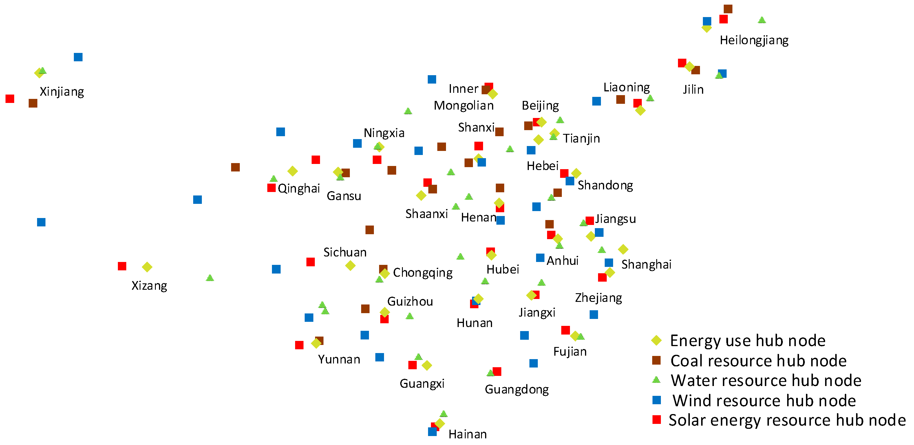
2. Determination of Geographical Location of Energy Supply and Use Hub Nodes

As one of the basic data of power network optimization, the distribution of energy supply and use hub nodes in China needs to be predicted first through a detail analysis. Based on national energy supply and use statistics [45], the geographical distribution of hub nodes of four main types of energy source, i.e., coal, solar energy, wind energy, and water energy, can be established.

2.1. Basic Method

In this work, the location of the main energy hub on the energy supplying/consumption side within the scope of the region are determined by Equations (1) and (2). As these equations show, by adding the potential energy supply/use amount Q predicted by statistics, the weight coefficient ω, and relevant coordinates at each node, and dividing by the potential energy supply/use amount of all nodes in the studied region, the latitude coordinate Cx and longitude coordinate Cy of the main energy supply/use hub nodes for each resources in the respective regions can be calculated.

$$C_x={\displaystyle \frac{{\displaystyle {\sum }_i^n{C}_{x,i}}·Q_i·{\omega }_i}{{\displaystyle {\sum }_i^n{Q}_i}}}$$

(1)

$$C_y={\displaystyle \frac{{\displaystyle {\sum }_i^n{C}_{\mathrm{y},i}}·Q_i·{\omega }_i}{{\displaystyle {\sum }_i^n{Q}_i}}}$$

(2)

where C_x,i and C_y,i are the latitude and longitude of the node i, respectively. Q_i is the potential amount of energy supply/use at the node i (kW). ω_i is the weight coefficient of the node i, and n is the total number of nodes in the considered region.

2.2. Geographical Distribution of Energy Supply Hub Nodes

2.2.1. Coal Resources

Based on the distribution of coal resources, the coordinate and energy data of 90 nodes at the city/county level were collected, and the coordinates of coal resource hubs were calculated according to the above-mentioned method. The detailed calculation results are listed in Appendix A 

Table A1. The 20 coal-resource hub nodes in China in 2020.

Province/City	Reserves (108 tons)	Longitude (°)	Latitude (°)
Beijing	2.66	115.5520	39.6650
Hebei	43.27	113.7625	39.2490
Shangxi	916.19	111.8173	37.1350
Neimeng	510.27	110.1176	38.2114
Liaoning	26.73	112.8835	42.0870
Jilin	9.71	126.0475	43.4540
Heiliongjiang	62.28	128.0715	47.6155
Anhui	82.37	116.8580	32.9425
Shandong	75.67	117.3716	35.0898
Henan	85.58	113.7733	35.3830
Hainan	1.19	109.7747	19.1877
Chongqing	18.03	106.4540	29.9010
Sichuan	53.21	105.5810	32.5490
Guizhou	110.93	105.3275	27.2105
Yunnan	59.58	102.4336	25.0382
Shaanxi	162.93	109.5455	35.3570
Gansu	27.32	104.0905	36.4370
Qinghai	12.39	97.1730	36.8218
Ningxia	37.45	107.0003	36.6217
Xinjiang	162.31	84.4719	41.1917

. It can be found that the coal resource density in north China is obviously higher than that in west China, and the southeast lacks energy supply hub nodes of coal resources.

2.2.2. Solar Energy

According to the statistic, our work collected the data of 727 city/county-level nodes in China. These nodes were divided into provincial regions, and 27 supply hub nodes of solar energy were obtained through the above-mentioned method. The detailed results are listed in Appendix A 

Table A2. The 27 solar-resource hub nodes in China in 2020.

Province/City	Theoretical Generating Capacity (1014 kWh)	Longitude (°)	Latitude (°)
Beijing/Tianjing/Hebei	3.224646	116.0782	39.9118
Shangxi	2.243232	112.4405	38.2721
Neimeng	17.28671	113.0702	42.3019
Liaoning	2.008588	122.3996	41.1839
Jilin	2.421405	125.1836	43.9146
Heiliongjiang	5.813514	127.7743	46.9314
Shanghai/Jiangsu	1.685354	119.4043	33.1718
Zhejiang	1.254029	120.1877	29.3330
Anhui	1.650294	116.9937	32.2194
Fujian	1.519828	117.8737	25.7658
Jiangxi	1.988142	115.9776	28.1739
Shandong	2.134186	117.7973	36.3849
Henan	2.128344	113.7414	34.0587
Hubei	2.177025	113.1811	31.0684
Hunan	2.408748	112.1432	27.5411
Guangdong	2.343515	113.5553	22.9223
Guangxi	2.766068	108.2855	23.3804
Hainan	0.463445	109.6606	19.165
Chongqing/Sichuan	7.165879	101.8854	30.4218
Guizhou	1.844045	106.5153	26.5120
Yunnan	5.621710	101.1811	24.7487
Tibet	22.98339	90.09129	30.1256
Shaanxi	2.532398	109.2059	35.7986
Gansu	6.523287	102.2071	37.3745
Qinghai	13.29972	99.41850	35.4423
Ningxia	1.062225	106.0558	37.3519
Xinjiang	25.34629	83.0180	41.4895

. From the data, it can be observed that southern Xinjiang, Ningxia, Inner Mongolia, and Shanxi have rich solar resources. Meanwhile, the solar energy resources in north Xinjiang, Shanxi, and southern Gansu are also relatively abundant. However, the solar energy resources in southwest China such as Sichuan are relatively poor.

2.2.3. Water Energy

China has about 14.3% of the world’s total water resources, which has huge development potential. Based on the distribution of available water resources in each region of the country, the data of 79 city/county-level resource nodes were collected, and 31 main water resource hub nodes in all regions have been found. The detailed values of the calculation results are listed in Appendix A 

Table A3. The 31 water-resource hub nodes in China in 2020.

Province/City	Reserves (108 m3)	Longitude (°)	Latitude (°)
Beijing	12.00	117.5588	40.0513
Tianjing	8.80	117.1171	38.9123
Hebei	60.00	114.4203	38.0915
Shangxi	87.80	110.6886	36.5396
Neimeng	194.10	108.0026	40.6843
Liaoning	161.00	123.1850	41.5388
Jilin	339.80	127.5406	43.0842
Heiliongjiang	626.50	130.2082	46.8707
Shanghai/Jiangsu	323.20	119.0226	33.0688
Zhejiang	881.90	120.1771	31.2082
Anhui	717.80	117.5140	31.5181
Fujian	1054.20	118.8065	25.3104
Jiangxi	1637.20	116.3918	29.0029
Shandong	139.10	117.0219	34.7939
Henan	311.20	111.7925	34.8207
Hubei	1219.30	111.2846	30.7292
Hunan	1905.70	112.8319	29.0996
Guangdong	1777.00	113.1769	22.8857
Guangxi	2386.00	108.6833	23.9132
Hainan	380.50	110.2425	20.1054
Chongqing	656.10	106.1997	29.2453
Sichuan	2466.00	102.6462	27.4700
Guizhou	1051.50	108.1130	26.7552
Yunnan	2202.60	102.8034	27.0470
Tibet	4749.90	95.5998	29.3096
Shaanxi	422.60	110.9940	34.1321
Gansu	231.80	103.7621	36.1671
Qinghai	764.30	99.5951	36.0251
Ningxia	8.70	106.1384	38.2543
Xinjiang	969.50	85.1164	43.4107

. Results show that the water resources are relatively evenly distributed in the whole country.

2.2.4. Wind Energy

In addition to water resources, China’s superior geographical and climate conditions create relatively rich wind resources. The data for calculating wind resources in this work are from 59 city/county-level nodes in China, and 27 wind energy supply hub nodes were identified. The detailed values of the calculation results are listed in Appendix A 

Table A4. The 27 wind-resource hub nodes in China in 2020.

Province/City	Theoretical Power (108 kW)	Longitude (°)	Latitude (°)
Beijing/Tianjing/Hebei	321.438197	115.7220	37.9880
Shangxi	193.6615	112.6320	37.1680
Neimeng	4086.0580	109.4982	42.8271
Liaoning	390.8169	119.8430	41.3150
Jilin	631.2966	127.6805	43.2225
Heiliongjiang	1429.701	126.7491	46.7967
Shanghai/Jiangsu	183.679	119.9900	32.3740
Zhejiang	67.38223	120.5867	30.3367
Anhui	159.7708	116.0650	34.1350
Fujian	50.66145	119.6480	26.8360
Jiangxi	98.82727	115.2900	25.3900
Shandong	302.6211	118.1510	35.8620
Henan	156.5264	113.8100	33.2050
Hubei	89.44367	116.2863	30.6830
Hunan	77.96374	112.2640	27.7670
Guangdong	154.8294	115.8675	23.5050
Guangxi	163.2147	106.2250	23.9225
Hainan	34.33998	109.4967	18.8767
Chongqing/Sichuan	179.0371	99.7425	29.9175
Guizhou	52.4084	105.2850	25.4450
Yunnan	193.5417	101.7770	26.6065
Tibet	2158.727	85.0147	33.1050
Shaanxi	129.4038	108.6650	37.9300
Gansu	656.4527	99.9950	39.2550
Qinghai	1264.5400	94.7903	34.6343
Ningxia	80.79878	104.8236	38.4762
Xinjiang	3528.9320	87.3124	44.3123

. It can be found that most of the wind resources are located in northern China, eastern coastal areas, and some areas of western China, while the wind resources are fewer in the central inland areas.

In summary, by means of the method introduced in Section 2.1, the geographical coordinates of the energy supply hub nodes of the above four resources in each province in China can be determined. The detailed calculated results from the above four energy sources of the energy supply hub nodes in each province are shown in

Table 1. Theoretical power generation from four energy sources of energy supply hub nodes in China (unit: 10⁸ kWh) [45].

Province/City	Coal	Solar	Water	Wind
Beijing	40.2834	113.8918	11.4763	6.0829
Tianjin	-		0.1669	10.0915
Hebei	655.2860		16.0928	164.3516
Shangxi	13,874.8862	79.2291	32.6802	108.7642
Neimeng	7727.5894	610.5521	67.0221	2294.8120
Liaoning	404.8023	70.9417	32.7416	219.4906
Jilin	147.0494	85.5220	52.0232	354.5488
Heiliongjiang	943.1757	205.3285	18.4838	802.9487
Shanghai	-	59.5250	20.8019	7.7368
Jiangsu	-			95.4209
Zhejiang	-	44.2913	366.9260	37.8432
Anhui	1247.4213	58.2870	90.5679	89.7304
Fujian	-	53.6791	701.4053	28.4525
Jiangxi	-	70.2195	322.5589	55.5034
Shandong	1145.9552	75.3777	15.9629	169.9580
Henan	1296.0334	75.1713	152.1022	87.9084
Hubei	-	76.8907	1809.8562	50.2333
Hunan	-	85.0750	846.7218	43.7860
Guangdong	-	82.7710	702.2210	86.9553
Guangxi	-	97.6952	1259.4223	91.6646
Hainan	18.0215	16.3685	9.3256	19.2860
Chongqing	273.0485	253.0928	348.2183	4.5412
Sichuan	805.8186		4700.9097	96.0096
Guizhou	1679.9374	65.1301	1387.2926	29.4336
Yunnan	902.2865	198.5541	3943.0686	108.6969
Tibet	-	811.7540	75.3651	1212.3841
Shaanxi	2467.4313	89.3971	220.7372	72.6758
Gansu	413.7373	230.3971	493.8871	368.6769
Qinghai	187.6357	469.7349	459.2729	710.1908
Ningxia	567.1472	37.5169	17.6687	45.3782
Xinjiang	2458.0414	930.5289	365.1824	1981.9191

. It should be pointed out that the absence of data in some blanks from Table 1 indicates that the relevant province is not the supply hub node of such energy source according to our calculations, which does not represent that such energy resources are not available in these regions.

It should be noted that the nuclear power plants are not being considered. This is based on the following considerations: firstly, our research aims to focus more on renewable energy, and it is generally agreed that nuclear power is not considered renewable energy; and secondly, more importantly, nuclear power plants are currently mainly distributed in coastal areas of China, not as widely distributed as the other resources considered in this section. Of course, we believe that nuclear power will be further considered in energy internet, when inland nuclear power plants can be gradually built and operated in the future.

2.3. Geographical Distribution of Energy Use Hub Nodes

Similar to the above methods, the calculation in this section is based on the social electricity consumption of cities/counties in China in 2020, and the corresponding coordinates of hub nodes on the energy use side are estimated.

Table A5. Annual electricity consumption in China in 2020.

Province/City	Electricity Consumption (108 kWh)	Longitude (°)	Latitude (°)
Beijing	1067	116.4000	39.9000
Tianjin	806	117.2000	39.1200
Hebei	3442	116.1948	38.7079
Shangxi	1991	112.4037	37.3669
Neimeng	2892	113.3114	41.7971
Liaoning	2135	122.5665	40.7352
Jilin	703	125.5946	43.6953
Heiliongjiang	929	126.7323	46.3745
Shanghai	1527	121.4700	31.2300
Jiangsu	5808	119.4758	32.1554
Zhejiang	4193	120.6236	29.6742
Anhui	1921	117.3997	31.9565
Fujian	2113	118.4834	25.3841
Jiangxi	1294	115.7359	28.0929
Shandong	5430	118.5676	36.4514
Henan	3166	113.6574	34.3753
Hubei	1869	113.2574	30.8349
Hunan	1582	112.4219	27.9361
Guangdong	5959	113.5609	22.8685
Guangxi	1442	109.1553	23.3798
Hainan	305	109.9758	19.4097
Chongqing	993	106.5500	29.5700
Sichuan	2205	104.3886	30.1842
Guizhou	1385	106.5823	26.9690
Yunnan	1538	102.2383	24.8396
Tibet	58	91.6423	30.0076
Shaanxi	1495	108.8434	34.9058
Gansu	1164	103.6010	36.5189
Qinghai	687	100.7710	36.5750
Ningxia	978	106.1654	38.2048
Xinjiang	2001	84.8932	43.2275

in the Appendix B lists the detailed data of annual electricity consumption by all provinces in 2020. Figure 1 shows the distribution of energy use hub nodes (highlighted with yellow rhombus) at the regional level obtained by calculation, and superposes the distribution of energy supply hub nodes of the four forms of energy sources obtained by previous analysis. In combination with the annual electricity consumption data of all provinces listed in Table A5 is the distribution diagram of main hub nodes on the energy use given in Figure 1.

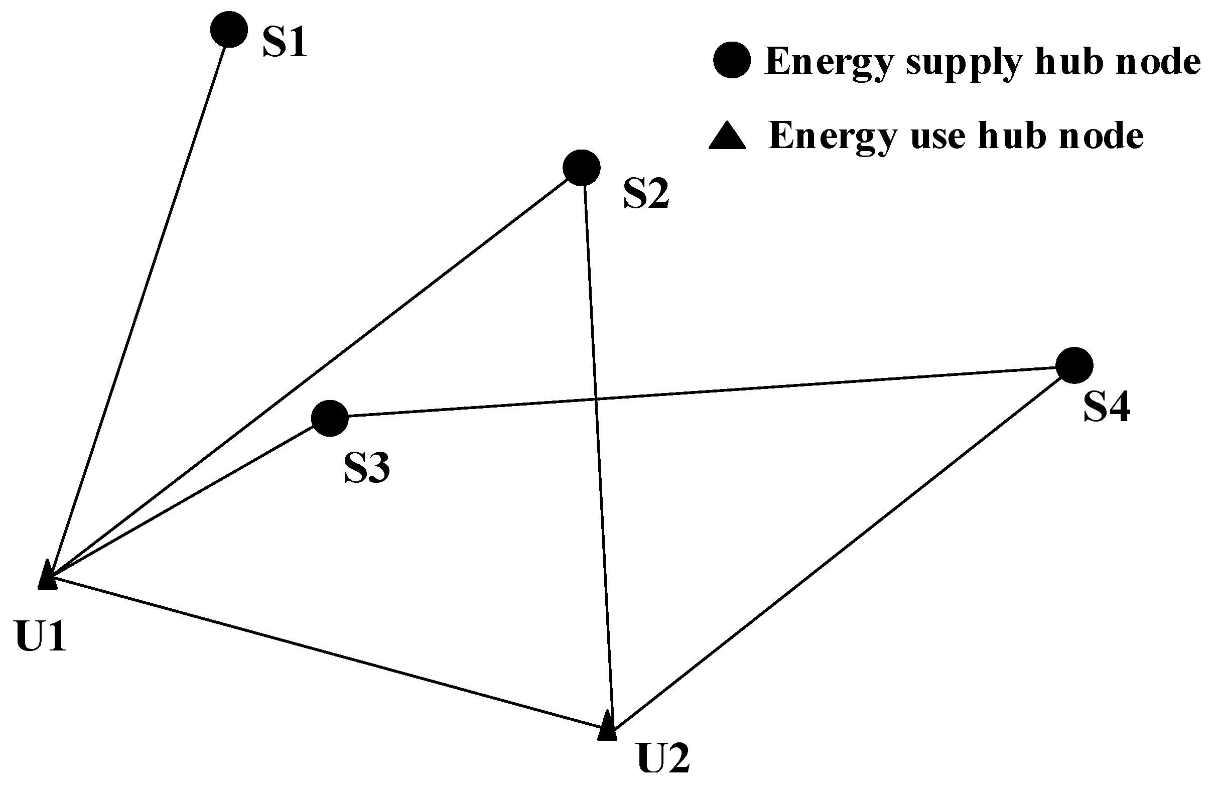
3. Synchronous Optimization Model

This section proposes a synchronous optimization model for optimizing the power network layout in China. The objective function of the proposed model is to minimize the total cost (TC) of the power network, which consists of the installation cost of power transmission line and power transmission cost. The optimization variables are both the length of transmission line and transmission capacity between different nodes. The specific concept and mathematical formula of the proposed model will be described below.

3.1. Model Description

According to the physical characteristics of the power network, the power network can be abstracted as the connection relation between various hub nodes in the network. Suppose there are N_s energy supply/use hub nodes in the region under consideration. Make any node i arbitrarily connected with other nodes in the region and ensure that each node is connected to at least one other node.

To be specific, there will be two kinds of matching relationships between energy supply and energy use hub nodes. The first is that a single energy supply hub node simultaneously provides power to several energy use hub nodes. The second is that an energy use hub node receives energy from one or more energy supply hubs. Moreover, if there is a connection between the energy supply hub nodes, an energy use hub node will also receive the energy from the energy supply hub node that is not directly connected to it. Take Figure 2, for example: the nodes directly connected with energy use hub node U1 are energy supply hub nodes S1, S2, and S3. However, U1 also receives energy from the energy supply hub node S4, which is connected to hub nodes S3 and U2. Meanwhile, the energy from hub node S2 feeds both nodes U1 and U2. In this case, energy transfer also occurs between the energy use hub nodes U1 and U2.

It should be pointed out that the form of energy transmission network considered in this work is direct current (DC) grids, which can achieve better inter-connection over large distances between energy sources and energy users as well as integration of large amounts of renewable sources [46,47]. Moreover, the numerous advantages of such configurations also include enhanced reliability, reduced converter station ratings, ease of maintenance, and energy trading facilitation [48,49].

Moreover, in order to reduce the difficulty of solving the model, the following assumptions are proposed:

• The maximum electric supply amount of each energy supply hub node and the maximum electric consumption of each energy use hub node are fixed values, which are calculated in Section 2 of this paper.
• The transmission voltages at both supply and use nodes are constant. Moreover, the technical requirements as well as the economics of different voltage levels are not considered.
• Only steady-state power transmission processes are considered.
• All physical properties of the transmission line connecting the two hub nodes are constant.
• The price of electricity is the average price of electricity in each region. The effect of peak-valley electricity price is not taken into account.
• The increase of load/use and the penetration of renewable energies or distributed resources are not considered.

3.2. Objective Function

As mentioned above, the optimization model was established by taking the total cost of transmission line (TC) as the objective function and can be calculated with Equation (3). It should be noted that the cost structure of a power grid network changes frequently [50]. To reduce the complexity of the model, we consider only the most basic cost here.

$$\min TC=F_{\mathrm{I},i,j}+F_{\mathrm{O},i,j}$$

(3)

where F_I,i,j represents the installation cost (CNY) of power transmission lines i-th and j-th hub nodes, including the cost of setting up transmission lines and the construction cost of auxiliary equipment such as pylons, substations, and relay stations. F_O,i,j represents the power transmission cost (CNY) between i-th and j-th hub nodes; here, the loss of transmission network transmission line is mainly considered.

The installation cost (CNY) of power transmission lines i-th and j-th hub nodes can be calculated as below:

$$F_{\mathrm{I},i,j}=\phi ·\epsilon ·m·d_{i,j}·f$$

(4)

where $\phi$ represents the conversion coefficient considering the expenses of auxiliary equipment such as towers and substations. $\epsilon$ represents the number of transmission line groups to be transmitted simultaneously. $m$ represents the mass of transmission line per unit length (kg/km). $d_{i,j}$ represents the length of transmission line between i-th and j-th hub nodes (km). $f$ represents the cost of transmission line per unit mass (CNY/kg).

Moreover, the power transmission cost between i-th and j-th hub nodes can be determined by the amount of transmission line energy loss, which is mainly affected by the maximum transmission current $I_{\max ,i,j}$ (A) and resistance in the transmission line $R_{i,j}$ (Ω). The specific formula is as follows:

$$F_{\mathrm{O},i,j}=I_{\max ,i,j}^2·R_{i,j}·s·t$$

(5)

$$I_{\max ,i,j}={\displaystyle \frac{P_i}{U_{i,j}}}$$

(6)

$$R_{i,j}={\displaystyle \frac{\rho ·d_{i,j}}{A_{i,j}}}$$

(7)

where s represents the price of electricity lost per unit (ca. 0.37628 CNY/kWh). t represents annual service hours (h/year); this paper assumes that the grid operates intermittently, i.e., 8760 h a year. $P_i$ represents the total electrical power transmitted to the network from the i-th hub node (kW). $U_{i,j}$ represents the supply voltage of transmission line between i-th and j-th hub nodes (kV). $\rho$ represents the resistivity of transmission line (Ω/m); this paper mainly considers transmission lines made of steel core aluminum stranded wire, and the electrical resistivity of such a transmission line is 2.83 × 10⁻⁸ Ω/m. $A_{i,j}$ represents the cross-sectional area of a transmission line between i-th and j-th hub nodes (m²). $d_{i,j}$ represents the length of transmission line between i-th and j-th hub nodes (m), which can be calculated with the following equation:

$$d_{i,j}=L·\arccos (\sin (y_i)·\sin (y_j)+\cos (y_i)·\cos (y_j)·\cos (x_i-x_j))$$

(8)

where L represents the radius of the earth, which is about 6371 km. x_i and x_j represent the longitude of i-th and j-th hub nodes, respectively. y_i and y_j represent the latitude of i-th and j-th hub nodes, respectively. It should be noted that the actual right-of-way distance for a transmission line in actual engineering is always longer than the calculated one, but the point-to-point distance suffices as an approximation.

To summarize, according to the model description in Section 3.1 and the above-mentioned equations, the objective function shown in Equation (3) can be further rewritten as:

$$\begin{array}{l}\min TC =\min {\displaystyle \sum _{j=1}^{N_{\mathrm{U}}}\begin{array}{l}[{\displaystyle \sum _{s=1}^{N{L}_{\mathrm{SU},j}}(\phi ·\epsilon ·m}·d_{\mathrm{s}, j}·f+{(\frac{P_{\mathrm{s}, j}}{U_{\mathrm{s}, j}})}^2 ·R_{\mathrm{s}, j}·s·t)+\\ {\displaystyle \sum _{\mathrm{z}=1}^{N{L}_{\mathrm{UU}, j}}(\phi ·\epsilon ·m}·d_{\mathrm{z}, j}·f+{(\frac{P_{\mathrm{z}, j}}{U_{\mathrm{z}, j}})}^2 ·R_{\mathrm{z}, j}·s·t)]\end{array}}\\ +{\displaystyle \sum _{i=1}^{N_{\mathrm{U}}}{\displaystyle \sum _{k=1}^{N_{\mathrm{SS},i}}(\phi ·\epsilon ·m·d_{k, i}·f+{(\frac{P_{k,i}}{U_{k,i}})}^2 ·R_{k,i}·s·t)}}\end{array}$$

(9)

The first part of the objective function represents the investment cost generated by the matching between energy supply and use hub nodes, and the second part represents the investment cost generated by the matching between two energy use hub nodes. Moreover, the third part is the investment cost generated by the connection between the different energy supply hub nodes. N_S and N_U are the total numbers of energy supply and use hub nodes in country, respectively. NL_SU,j, NL_UU,j and NL_SS,j are arrays representing the concrete connection relationship between supply and use hub nodes, between two energy use hub nodes, as well as between two energy supply hub nodes, respectively. The other symbols in Equation (9) have the same meaning as described above.

3.3. Constraint Conditions

3.3.1. Energy Flow Constraints

In order to ensure the electricity use of nodes, the energy transfer relation between different nodes can be described by the formula below:

$${\displaystyle \sum _{j=1}^{N_{\mathrm{U}}}({\displaystyle \sum _{s=1}^{N{L}_{\mathrm{SU}, j}}{P}_{s, j}}+ {\displaystyle \sum _{z=1}^{N{L}_{\mathrm{UU}, j}}{P}_{z, j}}- {\displaystyle \sum _{l=1}^{N{L}_{\mathrm{UU}, j}}{P}_{l, j}})}\ge P_{{\mathrm{U}}_j}$$

(10)

$${\displaystyle \sum _{i=1}^{N_S}({\displaystyle \sum _{k=1}^{N_{\mathrm{SS},i}}{P}_{k,i}})}+P_{S_{n,m}} \ge {\displaystyle \sum _{i=1}^{N_{\mathrm{S}}}({\displaystyle \sum _{s=1}^{N{L}_{\mathrm{SU},i}}{P}_{s,i}}+ {\displaystyle \sum _{q=1}^{N{L}_{\mathrm{UU},i}}{P}_{q,i}})}$$

(11)

$${\displaystyle \sum _{z=1}^{N{L}_{\mathrm{UU},j}}{\displaystyle \sum _{j=1}^{N_U}{P}_{j,z}}}> {\displaystyle \sum _{j=1}^{N_{\mathrm{U}}}{\displaystyle \sum _{z=1}^{N{L}_{\mathrm{UU},j}}{P}_{\mathrm{z},i}}}$$

(12)

Equation (10) represents the energy flow of the j-th energy use hub node. The first term represents the energy amount input from the s-th energy supply hub node into the j-th energy use hub node (kWh). The second term represents the energy amount transmitted from the z-th energy use hub node to the j-th energy use hub node (kWh). The third term represents the energy amount output from the j-th energy use hub node to the lth energy use hub node (kWh). Equation (11) means that the sum of the energy that a node obtains and the maximum energy amount that it can provide should be greater than or equal to the energy amount that this node transmits to other nodes. Equation (12) represents the energy flow between two energy use hub nodes.

3.3.2. Feasibility Constraints

Besides the energy flow, the constraint conditions need to consider the energy loss, maximum current limit, and the maximum resistance limit of the transmission line. Equations (13) and (14) describe the above constraints in detail.

$${\displaystyle \frac{P_{s,j}}{U_{s,j}}}\le I_{\max },\hspace{1em}\hspace{1em}s\in N{L}_{SU,j},j\in N_U$$

(13)

$${\displaystyle \frac{P_{z,j}}{U_{z,j}}}\le I_{\max },\hspace{1em}\hspace{1em}z\in N{L}_{UU,j},j\in N_S$$

(14)

where I_max represents the maximum direct current (A) in the transmission line, when the ambient temperature is 20 °C. P represents the total electrical power transmitted to the network from the j-th hub node (kWh). U represents the supply voltage of transmission line between two hub nodes (kV).

3.3.3. Penalty Constraints

The penalties for optimization are mainly divided into two categories:

First, it should be avoided that the energy output of the energy supply hub node exceeds its own capacity. Therefore, a penalty as shown in Equation (15) needs to be introduced.

$$L_1=| {\displaystyle \sum _{s=1}^{N{L}_{\mathrm{SU},j}}{\displaystyle \sum _{j=1}^{N_U}{P}_{s,i}}-}{P}_{\mathrm{S},\max }|·\mathsf{\Phi }$$

(15)

where P_S,_max represents the maximum energy amount that can be provided by the energy supply hub node (kWh).

Second, in order to ensure that the energy use hub can receive enough energy to meet its use, the algorithm takes 1.1 times the energy use as the threshold. If the energy transmitted to the energy use hub node is less than this threshold, a penalty constraint needs to be added to ensure that the energy use of hub nodes can be met. Such constraint is shown in Equation (16).

$$L_2=| ({\displaystyle \sum _{j=1}^{N{L}_{\mathrm{U}}}{\displaystyle \sum _{s=1}^{N{L}_{\mathrm{SU},j}}{P}_{j,s}}+{\displaystyle \sum _{j=1}^{N{L}_{\mathrm{U}}}{\displaystyle \sum _{l=1}^{N{L}_{\mathrm{UU},j}}{P}_{j,l}})-}1.1}\times P_{\mathrm{U},\max }|·\mathsf{\Phi }$$

(16)

where P_U,_max represents the maximum energy use of the energy use hub node (kWh) and Φ represents the penalty coefficient. In order to ensure the punishment effect, the punishment system for both equations above is set to 10¹⁰.

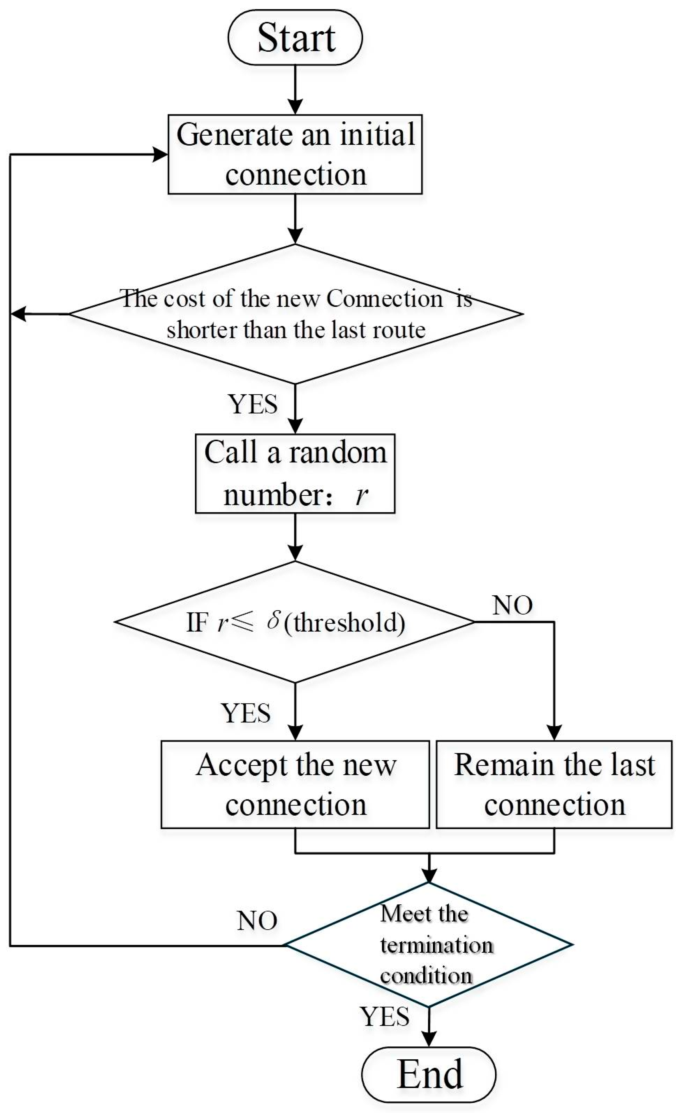
3.4. Model-Solving Strategy

The Random Walk algorithm with Compulsive Evolution (RWCE), as developed by our research group, is used to solve the established model. The general flow chart of applying the RWCE to optimize the established model is shown in Figure 3 and each specific step is described in the following sections. It should be noted that all the model-solving process in this paper is implemented through the Fortran programming language (Version 6.6) and the computer used is the Intel(R) Core (TM) i5-7200U CPU@ 2.50 GHz 2.70 GHz.

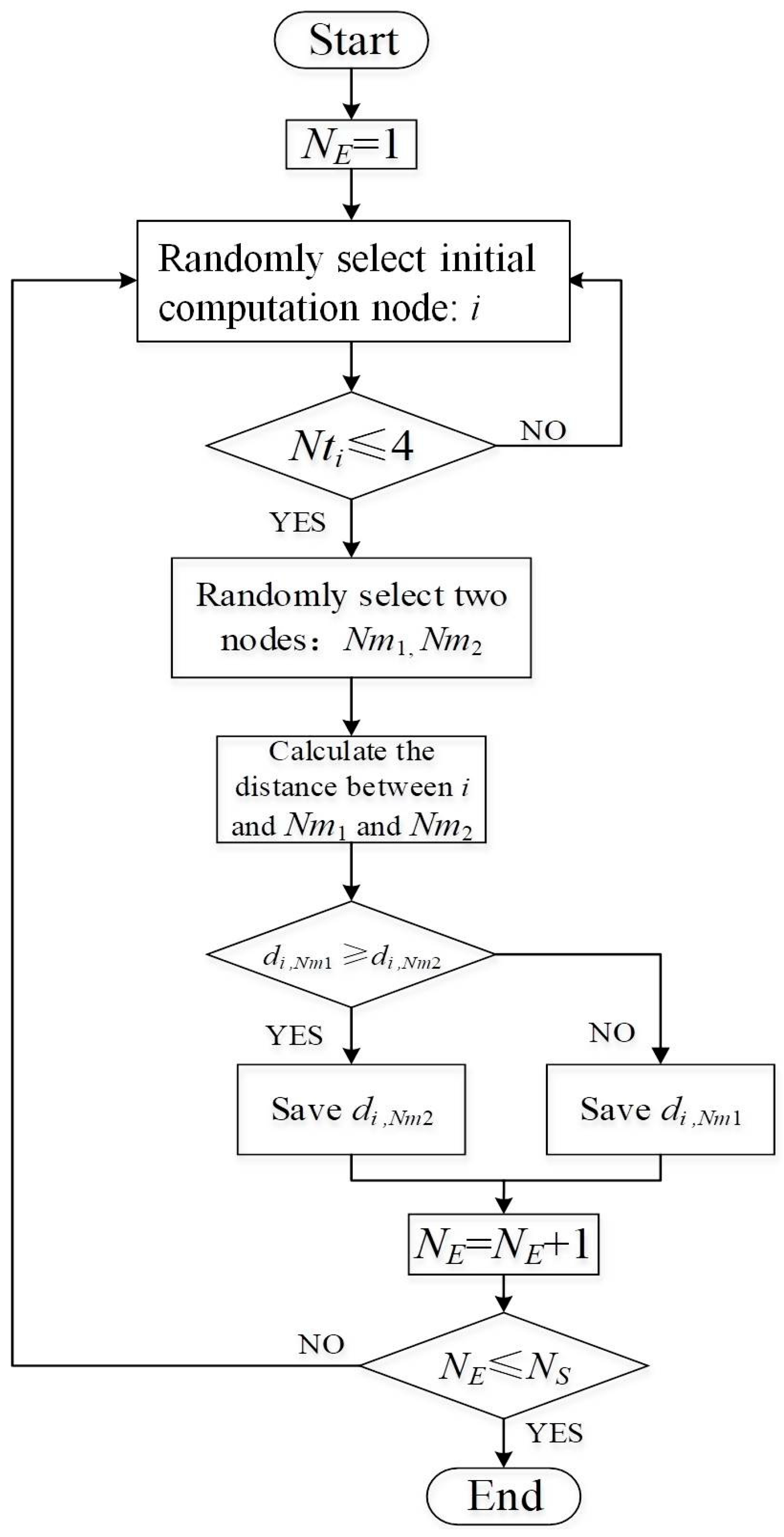
3.4.1. Initialization

As shown in Equations (17) and (18), the initial population M, which contains NN individuals, is randomly generated, and each individual corresponds to a network structure. Take the electric amount P (kWh) as optimization variable, and the number of variables in each dimension is NS.

$$M={\left[P_1,P_2,P_3,\dots ,P_{NN}\right]}^{\mathrm{T}}$$

(17)

$$P_{nn}=\left[P_{nn,1},P_{nn,2},P_{nn,3},\dots ,P_{nn,NS}\right],\hspace{1em}\hspace{1em}nn=1,2,\dots ,NN$$

(18)

In the initialization process, several groups of connections are randomly generated in the network, and the number of three types of connections (i.e., supply–use (N_SU), supply–supply (N_SS), and use–use (N_UU) hub nodes) are counted, respectively. Afterwards, the existing connection is randomly endowed with electric amount, and the method of electric amount assignment is as follows:

$$P_{\mathrm{SU}}=P_{\mathrm{SU},\max }·{\left[{\alpha }_1,{\alpha }_2,\dots ,{\alpha }_{N_{\mathrm{SU}}}\right]}^{\mathrm{T}},\alpha \in (0,1)$$

(19)

$$P_{\mathrm{SS}}=P_{\mathrm{SS},\max }·{\left[{\beta }_1,{\beta }_2,\dots ,{\beta }_{N_{\mathrm{SS}}}\right]}^{\mathrm{T}},\beta \in (0,1)$$

(20)

$$P_{\mathrm{UU}}=P_{\mathrm{UU},\max }·{\left[{\gamma }_1,{\gamma }_2,\dots ,{\gamma }_{N_{\mathrm{UU}}}\right]}^{\mathrm{T}},\gamma \in (0,1)$$

(21)

where P_SU, P_SS, and P_UU are the total electric amounts (kWh) of three types of connections, i.e., supply–use, supply–supply, and use–use, respectively. P_SU,max, P_SS,max, and P_UU,max are their corresponding solution domains. α, β, and γ are pseudo random numbers generated, and are in the range of (0,1).

3.4.2. Evolution

The individual P_nn was randomly increased or decreased in each dimension, according to the following equations:

$${(P_{\mathrm{SU},nn}^{\prime })}_{it+1}={(P_{\mathrm{SU},nn})}_{it}+\Delta P_{\mathrm{SU},nn}=\left[\begin{array}{c}{P}_{nn,1}\\ P_{nn,1}\\ ⋮\\ P_{nn,1}\end{array}\right]+{\left[\begin{array}{c}(1-2{\rho }_1)·{\zeta }_1·\Delta L\\ (1-2{\rho }_2)·{\zeta }_2·\Delta L\\ ⋮\\ (1-2{\rho }_{N_{\mathrm{SU}}})·{\zeta }_{N_{\mathrm{SU}}}·\Delta L\end{array}\right]}^{\mathrm{T}}$$

(22)

$${(P_{\mathrm{SS},nn}^{\prime })}_{it+1}={(P_{\mathrm{SS},nn})}_{it}+\Delta P_{\mathrm{SS},nn}=\left[\begin{array}{c}{P}_{n,1}\\ P_{n,1}\\ ⋮\\ P_{n,1}\end{array}\right]+{\left[\begin{array}{c}(1-2{\rho }_1)·{\zeta }_1·\Delta L\\ (1-2{\rho }_2)·{\zeta }_2·\Delta L\\ ⋮\\ (1-2{\rho }_{N_{\mathrm{SS}}})·{\zeta }_{N_{\mathrm{SS}}}·\Delta L\end{array}\right]}^{\mathrm{T}}$$

(23)

$${(P_{\mathrm{UU},nn}^{\prime })}_{it+1}={(P_{\mathrm{UU},nn})}_{it}+\Delta P_{\mathrm{UU},nn}=\left[\begin{array}{c}{P}_{nn,1}\\ P_{nn,1}\\ ⋮\\ P_{nn,1}\end{array}\right]+{\left[\begin{array}{c}(1-2{\rho }_1)·{\zeta }_1·\Delta L\\ (1-2{\rho }_2)·{\zeta }_2·\Delta L\\ ⋮\\ (1-2{\rho }_{N_{\mathrm{UU}}})·{\zeta }_{N_{\mathrm{UU}}}·\Delta L\end{array}\right]}^{\mathrm{T}}$$

(24)

where (P_n)_it represents the amount of electricity obtained after the it-th iteration, and (P_n’)_it+1 represents the amount of electricity obtained after the (it + 1)th iteration. The evolution direction of the algorithm is determined by two random numbers ρ and ζ, which are uniformly evaluated on (0,1), and expressed as (1–2ρ)·ζ in the above equations. ΔL represents evolution step length.

3.4.3. Selection and Variation

The selection process mainly determines whether a variable can be involved in the subsequent optimization process according to the set threshold. Equations (23)–(25) represent the selection scheme of electric amount of transmission in three different connection types, respectively:

$${(P_{\mathrm{SU},nn})}_{it+1}=\{\begin{array}{l}{(P_{\mathrm{SU},nn})}_{it+1}^{″}, \mathrm{if}{(P_{\mathrm{SU},nn})}_{it+1}^{″}\ge P_{\mathrm{SU},\mathrm{fix}}\\ 0\hspace{1em}\hspace{1em}\hspace{1em}\hspace{1em}\hspace{1em}, \mathrm{else}\end{array}$$

(25)

$${(P_{\mathrm{SS},nn})}_{it+1}=\{\begin{array}{l}{(P_{\mathrm{SS},nn})}_{it+1}^{″}, \mathrm{if}{(P_{\mathrm{SS},nn})}_{it+1}^{″}\ge P_{\mathrm{SS},\mathrm{fix}}\\ 0\hspace{1em}\hspace{1em}\hspace{1em}\hspace{1em}\hspace{1em},\mathrm{else}\end{array}$$

(26)

$${(P_{\mathrm{UU},nn})}_{it+1}=\{\begin{array}{l}{(P_{\mathrm{UU},nn})}_{it+1}^{″}, \mathrm{if}{(P_{\mathrm{UU},nn})}_{it+1}^{″}\ge P_{\mathrm{UU},\mathrm{fix}}\\ 0\hspace{1em}\hspace{1em}\hspace{1em}\hspace{1em}\hspace{1em},\mathrm{else}\end{array}$$

(27)

where P_SU,fix, P_SS,fix, and P_UU,fix are thresholds (kWh) of electric amount in the above-mentioned three connection types, which are set according to the minimum power supply capacity in each province.

Furthermore, since the goal of the RWCE algorithm is to reduce the TC of the power network, when the TC of the (it + 1)th iteration is lower than the TC obtained in the previous step, the variables can be updated. In order to enhance the global search capability of the algorithm and avoid the dilemma of local optimal solution, the mechanism of accepting bead solutions is also retained. In other words, when the calculated TC of the new structure after evolution is higher than the TC calculated in the previous step, the algorithm can still accept this solution with a small probability, as shown in the following equation:

$${(P_{nn})}_{it+1}=\{\begin{array}{l}{(P_{nn})}_{it+1}^{″}, \mathrm{if} F({(P_{nn})}_{it+1}^{″})\le F({(P_{nn})}_{it+1})\\ {(P_{nn})}_{it+1}^{″}, \mathrm{else} \mathrm{if}(r<\delta )\\ {(P_{nn})}_{it+1}, \mathrm{else}\end{array}$$

(28)

where r is a uniformly distributed random number from 0 to 1.

3.4.4. Terminate the Iteration

When the optimization result does not change significantly over 10,000 iterations (the relative changes of all iteration results are less than 10⁻⁶), the iteration is terminated, and the optimization results are displayed. If not, the step described in Section 3.4.2 is repeated, and the iteration continues until the termination condition is satisfied.

4. Results and Discussions

This section compares the results of the proposed synchronous optimization method (i.e., the transmission line length and transmission capacity between nodes are optimized simultaneously) with those of optimizing only the transmission line length. In order to ensure sufficient comparability, the RWCE algorithm is also used for optimization that only uses the length of transmission line as an optimization variable. Considering the length of the paper, please refer to the Appendix C for the detailed process of the latter. Moreover, the results will be compared from three networks of different scales, i.e., municipal, provincial, and national, to verify the superiority of synchronous optimization.

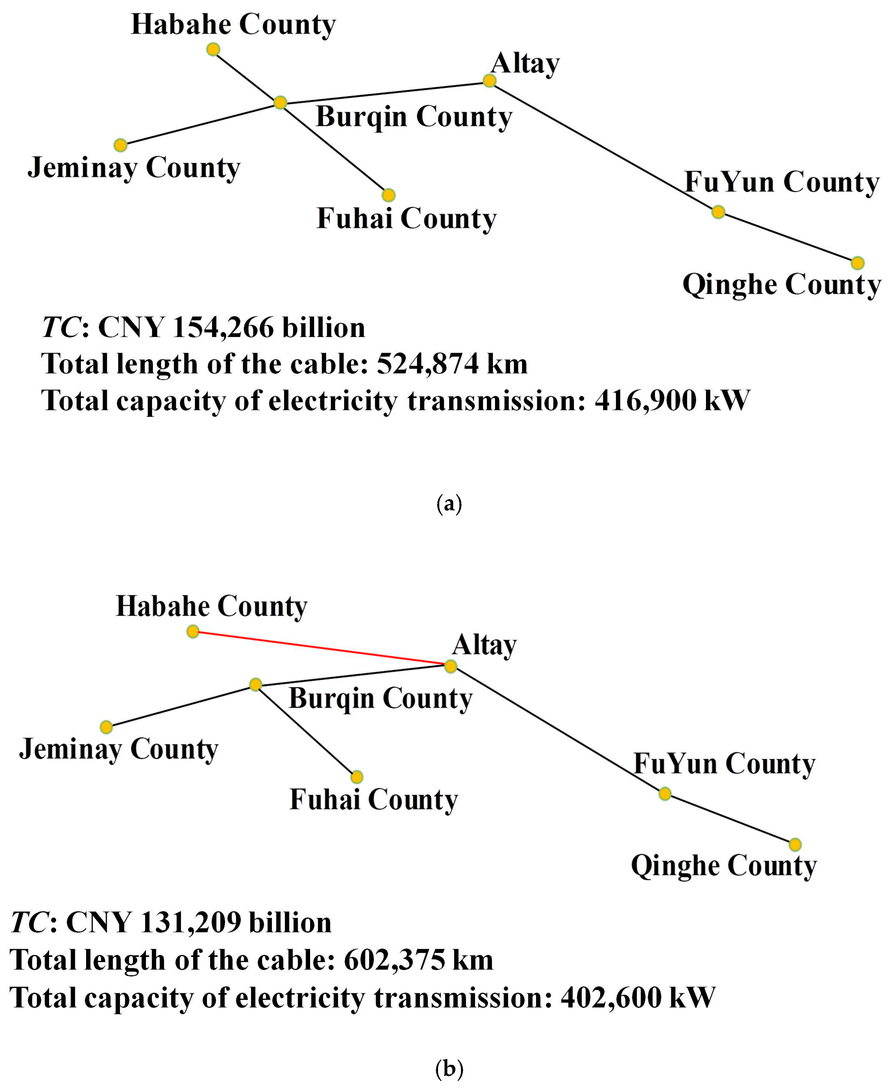
4.1. Optimal Layout of Municipal Power Network

Firstly, taking the Altay city in Xinjiang as an example, the optimization results of municipal power network are analyzed. The geographical longitude of the city is 88.13°, and the latitude is 47.85°. The city’s annual electricity consumption is 545,270 kWh. As can be seen from Figure 4, the municipal power network of Altay consists of one city-level node and six county-level nodes subordinate to the city. Figure 4a is the optimization result only focused on transmission line length, while Figure 4b is the result of synchronous optimization.

From the point of view of route direction, the only difference between the two results is the connection between Altay City and Habahe County. The former chose to establish a connection between the Habahe and Burqin counties rather than between Habahe County and Altay City, to reduce the overall length of the transmission line. Such planning, however, can lead to a higher TC. It can be found in Figure 4 that although the direct transmission of electricity from Altay City to Habahe County would increase the length of transmission line by 7,749,367 km, such planning reduced the power transmission by 14,300 kW, thus saving CNY 230.60 million in TC. In other words, while the results obtained through synchronous optimization will increase the initial investment cost of the network, the operating cost will decrease significantly, resulting in a decrease in the TC.

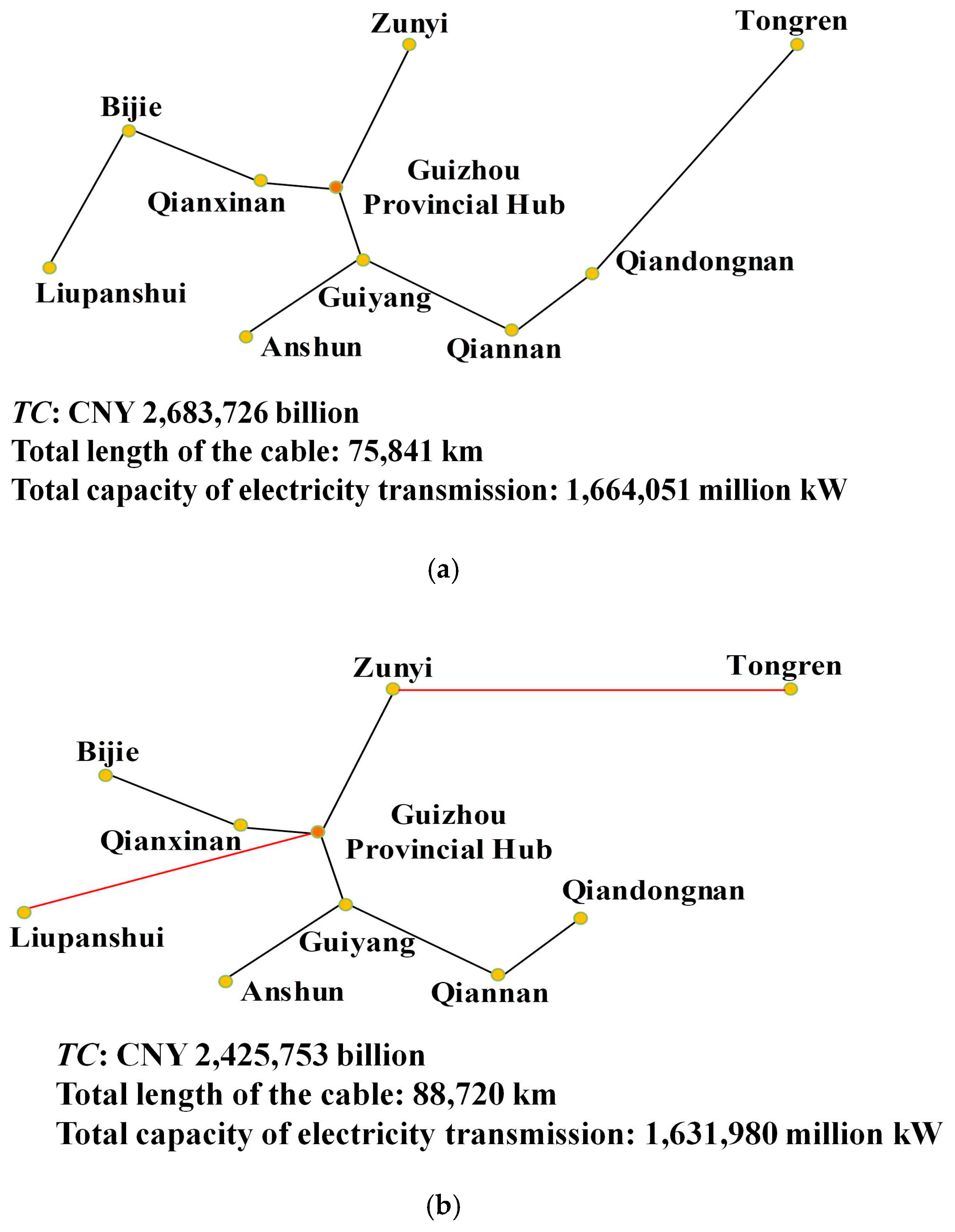
4.2. Optimal Layout of Provincial Power Network

After verifying the optimization results of municipal networks, this section applies the proposed algorithm to larger scale network optimization, and takes Guizhou province as an example to verify the applicability of this method in provincial power network optimization. The network in Guizhou province consists of one provincial hub node and nine municipal hub nodes. Figure 5a,b show the optimization results with two different methods. By comparing the two figures, it can be found that, different from the algorithm that only optimizes the transmission line length, the synchronous optimization algorithm proposes to establish the connection between Zunyi City and Tongren City, while cancelling the connection between Qiandongnan City and Tongren City. Moreover, the strategy also suggests establishing a connection between Guizhou provincial hub node and Liupanshui city nodes, while eliminating the connection between Bijie City and Liupanshui City. Through the above improvements, although the total length of the transmission line is increased by 128.79 km, the TC of the network can be reduced by CNY 2.58 billion.

Taking the Liupanshui city at the end of the connection route as an example, when only the transmission line length is considered, the electricity amount required can only be transmitted to this node from the Guizhou provincial hub node after passing through Bijie City and Qianxinan City. Its total transmission energy loss will include the loss of three sections of the connections, much larger than the direct transmission from the Guizhou provincial hub node to Liupanshui City.

To further verify the superiority of the proposed method in improving power network economy,

Table 2. Comparison of optimization results on provincial power network.

Province	Optimizing the Length Only		Synchronous Optimization		Cost Saving
	FI (108 CNY)	FO (108 CNY/a)	FI (108 CNY)	FO (108 CNY/a)	ΔTC Over a 30-Year Operating Period (108 CNY)
Hebei	935.16	42.597	949.579	39.128	89.651
Shanxi	461.173	29.212	463.874	27.932	35.699
Neimeng	1643.459	57.967	1798.906	43.046	292.183
Jilin	143.186	11.396	161.696	4.339	193.2
Heilongjiang	373.235	17.279	386.849	6.728	302.916
Jiangsu	984.131	91.06	985.027	88.867	64.894
Zhejiang	652.097	82.2	653.259	73.649	255.368
Anhui	407.546	37.963	412.632	28.756	271.124
Fujian	343.38	41.726	344.251	35.997	170.999
Jiangxi	285.255	24.571	300.514	19.695	131.021
Shandong	1251.312	64.086	1255.622	62.672	38.11
Hubei	559.133	23.549	597.83	17.361	146.943
Guangdong	674.446	43.449	710.088	37.435	144.778
Ningxia	86.156	19.185	93.08	16.396	76.746
Sichuan	887.824	41.417	923.337	39.431	24.067
Yunnan	633.238	30.338	701.377	25.98	62.601
Shaanxi	460.92	29.243	511.983	26.756	23.547
Hunan	327.89	29.327	332.084	21.085	243.066
Liaoning	408.671	28.922	436.321	27.333	20.02
Tibet	92.473	1.088	92.473	1.088	0
Guizhou	223.138	21.714	268.373	16.788	102.545
Gansu	401.086	20.688	401.593	19.386	38.553
Guangxi	355.592	28.522	376.532	23.752	122.16
Henan	596.156	62.21	600.56	42.515	586.446
Xinjiang	1026.656	39.8	1162.424	31.779	104.862

lists the optimization results of 25 provincial networks in China. The TC savings after 30 years of operation with synchronous optimization are listed in the last column of the table. It can be seen from the table that adopting synchronous optimization plays an obvious role in improving the economy of provincial networks. The main reason why the proposed method has no influence on the optimization results in Tibet is that the number of nodes in the network is too small for further optimization.

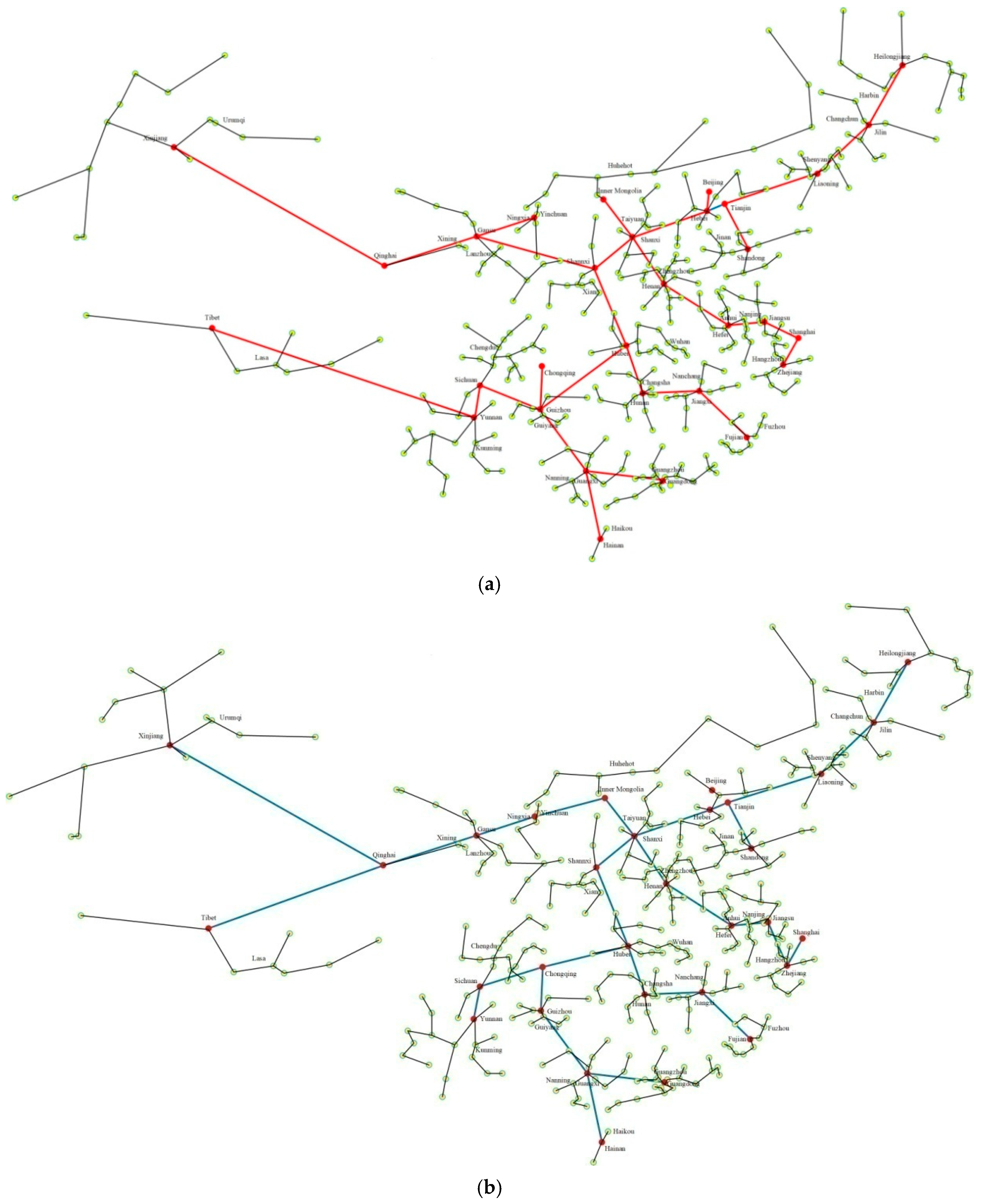
4.3. Optimal Layout of National Power Network

In this section, the hub nodes in 25 provincial power networks are optimized synchronously to explore the possibility of the recommended method for improving the economy of the national network in China. The network (Figure 6) contains 126 nodes and the required computation time is ca. 150,000 s. Figure 6a,b show the results of the length only and synchronous optimization methods, respectively. The color lines are connections between hub nodes of different provincial networks, while the lack lines are connections between different hub nodes within a provincial network. Energy supply hub nodes are shown in red and energy use nodes in yellow. The detailed data on the costs of inter-network connections at each provincial network are listed in

Table 3. The detailed data on the costs of inter-network connections at each provincial network.

Connections	Transmission Line Length (km)	Transmission Capacity (104 kW)	Voltage (kV)	Transmission Line Type (number × mm2)	Conversion Coefficient φ
Xinjiang–Qinghai	1307.338	4142.580	1000	6 × 630	66.4097
Tibet–Sichuan	1551.299	2327.183	1000	6 × 630	66.4097
Qinghai–Gansu	512.964	5122.507	1000	6 × 630	66.4097
Gansu–Shaanxi	648.010	4880.241	1000	6 × 630	66.4097
Shaanxi–Shanxi	281.223	7214.146	1000	6 × 630	66.4097
Neimeng–Shanxi	285.185	8737.356	1000	6 × 630	66.4097
Hubei–Shanxi	540.611	1063.445	1000	6 × 630	66.4097
Guizhou–Hubei	640.620	4685.388	1000	6 × 630	66.4097
Sichuan–Guizhou	376.310	10,203.601	1000	6 × 630	66.4097
Yunnan–Sichuan	209.373	4034.224	1000	6 × 630	66.4097
Heilongjiang–Jilin	421.663	1135.864	1000	6 × 630	66.4097
Gansu–Ningxia	322.887	426.751	500	6 × 630	37.7957
Guizhou–Chongqing	286.314	431.861	500	6 × 630	37.7957
Shanxi–Hebei	412.146	11,101.509	1000	6 × 630	66.4097
Hebei–Beijing	133.726	1172.642	500	4 × 630	45.0535
Hebei–Tianjin	98.302	6660.212	1000	6 × 630	66.4097
Tianjin–Shandong	320.137	4873.526	1000	6 × 630	66.4097
Tianjin–Liaoning	491.480	746.398	500	4 × 630	44.4825
Jilin–Liaoning	412.883	1008.031	1000	6 × 630	45.0535
Shanxi–Henan	349.069	18,286.997	1000	6 × 630	66.4097
Henan–Anhui	440.24	15,973.815	1000	6 × 630	66.4097
Anhui–Jiangsu	196.897	14,979.990	1000	6 × 630	66.4097
Jiangsu–Shanghai	214.907	8062.977	1000	6 × 630	66.4097
Shanghai–Zhejiang	191.075	6279.415	1000	6 × 630	66.4097
Hubei–Hunan	324.772	3660.007	1000	6 × 630	66.4097
Hunan–Jiangxi	325.779	2805.578	1000	6 × 630	66.4097
Jiangxi–Fujian	406.373	1703.876	1000	6 × 630	66.4097
Guangxi–Hainan	449.549	300.801	500	4 × 630	45.0535
Guizhou–Guangxi	483.333	6822.137	1000	6 × 630	66.4097
Guangxi–Guangdong	454.979	6251.526	1000	6 × 630	66.4097
Total investment cost FI (1012 CNY)					2.134
Annual operating cost Fo/a (1012 CNY/a)					0.115
Total cost over a 30-year operating period TC(30) (1012 CNY)					5.584

.

By comparing the data listed in

Table 4. Optimization results of inter-network connections in national power network.

Method	Transmission Line Length (km)	Transmission Capacity (104 kW)	FI (1012 CNY)	FO/a (1012 CNY/a)	TC(30) (1012 CNY)
I	12,204.681	163,395.003	2.073	0.123	5.763
II	13,089.440	165,094.583	2.134	0.115	5.584

I: Optimizing transmission line length only; II: Synchronous optimization.

, it can be found that although synchronous optimization cannot guarantee the shortest total length of transmission transmission lines, resulting in the increase in initial investment cost FI of the network, the operation cost of the network can be greatly reduced through the reasonable allocation of transmission capacity between provincial hub nodes. As can be seen from Figure 6b, connecting several provincial hub nodes with large energy supply amounts such as Xinjiang, Tibet, Neimeng, and Shanxi to supply power to the eastern region will significantly reduce the operation cost of the total power network. If the operation period of 30 years is considered, the saving of power network total cost is 1.79 × 1011 CNY.

4.4. Discussions

The above results are obtained by taking the total cost of transmission line of the energy transmission network as the optimization objective and the energy flow balance and feasibility of the network as the model constraints. According to the author’s preliminary literature survey, the above optimization results can demonstrate certain advantages in comparison with other research endeavors. For example, in reference [51], the economic optimization of China’s power grid was carried out by introducing a macro-level integrated source–grid–load planning model. The overall concept proposed by the author was similar to our work, which is to introduce high voltage transmission to perform the long-distance transmission of electric power due to its advantages in transmission capacity, transmission distance, and line loss rate. The research results show that among the three scenarios they proposed, the lowest total cost of national power grid was ca. 4.1 × 1013 CNY. Moreover, a multi-objective optimization model for transmission line layout is established in reference [37] to improve the cross-regional consumption of renewable power in China. The lowest total cost appears in Scenario L-TS of the seven proposed solutions, which was ca. 9.5 × 10¹² CNY. These values are significantly higher than the optimization results of the cost listed in Table 4.

It should be noted that power network layout not only considers the investment, but also its reliability. The configuration provided in this work only considers the radial topology of the power network. For the development of large-scale meshed DC grids at present, there are still several technical and non-technical barriers that need to be overcome, such as the protection of the lines and control of the network [48]. The existing literature has reported that modular multi-level converters (MMCs) are well-suited for DC grids due to their several advantages [52,53]. Several investigations have been conducted on different aspects of voltage-sourced converter (VSC)-based DC networks such as coordinated control [54,55] and protection strategies for continued operation during AC and DC network faults [52]. In addition, the master–slave control method proposed in [56] minimizes the risk of the conventional control method by quickly reallocating the distributed DC voltage control function to a new converter. The droop control method in [57] permits the participation of multiple converters to DC grid voltage regulation and is appreciated for its stability and resiliency to converter outage. In recent years, several series of current/power flow controllers have been proposed in order to prevent DC line overload through the manipulation of the DC line voltage drops based on predefined set-points or criteria [58,59]. The effectiveness of these controllers has been tested and validated. However, additional costs and space are needed. The above research provides many good perspectives for further improving the feasibility and reliability of the proposed configuration in our work. Considering the length of the paper and scope of the research, there will be no further in-depth discussion on network control here.

5. Conclusions

To improve cross-regional power transmission and the economy of China’s power network, a synchronous optimization method based on the Random Walk algorithm with Compulsive Evolution (RWCE) was proposed in this paper. The detail optimization steps and mathematical model are introduced. The advantages of the proposed method are verified in the optimization of power network for multiple scales. The following are the main conclusions of the research:

• The geographical coordinates and potential energy amounts of the coal, solar, water, and wind energy supply hub nodes in China are calculated in detail, and used as the basic data for subsequent optimization.
• A synchronous optimization model of the multi-scale power network in China is proposed, which takes the length of transmission lines and the power transmission between different nodes as the optimization variables, and the total cost of the network as the optimization objective. The RWCE was used to solve the established model to better approximate the global optimal solution of the problem.
• Results of optimization by the synchronous method show that, compared with the optimization method that only optimizes the transmission line length, although the proposed method will cause a slight increase in investment cost, it can obviously reduce the operating cost of the network, so as to bring a significant improvement in network economy on the basis of ensuring the balance between power supply and use.
• Taking Altay City and Guizhou Province as examples for municipal and provincial power networks, the saving of total annual cost of power network optimized by the proposed method is CNY 230.60 million and CNY 2.58 billion, respectively. Moreover, for the nationwide power network, the total cost savings over 30 years of operation amount to CNY 179 billion.

It should be pointed out that there are a lot of factors involved in national power network planning. As this article is a preliminary study for feasibility analysis, only the main influencing factors are analyzed in the model, and the influence of other factors such as geographical and environmental conditions on power grid construction are not considered. Moreover, we acknowledge that the cost increase caused by the renovation factors of the existing power grid and the impact on the feasibility of the optimization results were not considered in the study. Taking these aspects into account will help the proposed method continuously improve in the future.

References

1. Wang, Z.; Zheng, H.; Pei, L.; Jin, T. Decomposition of the factors influencing export fluctuation in China’s new energy. Energy Policy 2017, 109, 22–35. [Google Scholar] [CrossRef]
2. Liu, S.; Lin, Z.; Jiang, Y.; Zhang, T.; Yang, L.; Tan, W.; Lu, F. Modelling and discussion on emission reduction transformation path of China’s electric power industry under “double carbon” goal. Heliyon 2022, 8, 10497. [Google Scholar] [CrossRef] [PubMed]
3. Xu, M.; Tan, R. How to reduce CO2 emissions in pharmaceutical industry of China: Evidence from total-factor carbon emissions performance. J. Clean. Prod. 2022, 337, 130505. [Google Scholar] [CrossRef]
4. Yao, X.; Fan, Y.; Zhao, F.; Ma, S. Economic and climate benefits of vehicle-to-grid for low-carbon transitions of power systems: A case study of China’s 2030 renewable energy target. J. Clean. Prod. 2022, 330, 129833. [Google Scholar] [CrossRef]
5. Zeng, S.; Su, B.; Zhang, M.; Gao, Y.; Liu, J.; Luo, S.; Tao, Q. Analysis and forecast of China’s energy use structure. Energy Policy 2021, 159, 112630. [Google Scholar] [CrossRef]
6. Solarin, S.; Bello, M.; Tiwari, A. The impact of technological innovation on renewable energy production: Accounting for the roles of economic and environmental factors using a method of moments quantile regression. Heliyon 2022, 8, 09913. [Google Scholar] [CrossRef]
7. Mao, Y. China’s Transmission Trunk Line Layout Optimization: Considering Renewable Energy Development and Transmission Technology Selection; China University of Geoscience: Wuhan, China, 2019. (In Chinese) [Google Scholar]
8. Quitzow, R.; Huenteler, J.; Asmussen, H. Development trajectories in China’s wind and solar energy industries: How technology-related differences shape the dynamics of industry localization and catching up. J. Clean. Prod. 2017, 158, 122–133. [Google Scholar] [CrossRef]
9. Kurukuru, V.S.; Haque, A.; Khan, A.; Blaabjerg, F. Resource management with kernel-based approaches for grid-connected solar photovoltaic systems. Heliyon 2021, 7, 08609. [Google Scholar] [CrossRef]
10. Kha, M.; Zahedi, R.; Eskandarpanah, R.; Mirzaei, A.; Farahani, O.; Malek, I.; Rezaei, N. Optimal sizing of residential photovoltaic and battery system connected to the power grid based on the cost of energy and peak load. Heliyon 2023, 9, 14414. [Google Scholar]
11. Quelhas, A.; Gil, E.; McCalley, J.D.; Ryan, S.M. A multiperiod generalized network flow model of the U.S. integrated energy system: Part I—Model description. IEEE Trans. Power Syst. 2007, 22, 829–836. [Google Scholar] [CrossRef]
12. Quelhas, A.; McCalley, J.D. A multiperiod generalized network flow model of the U.S. integrated energy system: Part II—Simulation results. IEEE Trans. Power Syst. 2007, 22, 837–844. [Google Scholar] [CrossRef]
13. Unsihuay, L.; Marangon-Lima, J.W.; de Souza, A.C.Z. Integrated power generation and natural gas expansion planning. In Proceedings of the IEEE Power Tech Conference, Lausanne, Switzerland, 1–5 July 2007; pp. 1404–1409. [Google Scholar]
14. Adetokun, B.; Muriithi, C. Application and control of flexible alternating current transmission system devices for voltage stability enhancement of renewable-integrated power grid: A comprehensive review. Heliyon 2021, 7, 06461. [Google Scholar] [CrossRef] [PubMed]
15. Sharan, I.; Balasubramanian, R. Integrated generation and transmission expansion planning including power and fuel transportation constraints. Energy Policy 2012, 43, 275–284. [Google Scholar] [CrossRef]
16. Wang, C.; Ye, M.; Cai, W.; Chen, J. The value of a clear, long-term climate policy agenda: A case study of China’s power sector using a multi-region optimization model. Appl. Energy 2014, 25, 276–288. [Google Scholar] [CrossRef]
17. Guo, Z.; Ma, L.; Liu, P.; Jones, I.; Li, Z. A multi-regional modelling and optimization approach to China’s power generation and transmission planning. Energy 2016, 116, 1348–1359. [Google Scholar] [CrossRef]
18. Yi, B.; Xu, J.; Fan, Y. Inter-regional power grid planning up to 2030 in China considering renewable energy development and regional pollutant control: A multi-region bottom-up optimization model. Appl. Energy 2016, 184, 641–658. [Google Scholar] [CrossRef]
19. Zhang, Y.; Ma, T.; Guo, F. A multi-regional energy transport and structure model for China’s electricity system. Energy 2018, 161, 907–919. [Google Scholar] [CrossRef]
20. Wang, H.; Su, B.; Mu, H.; Li, N.; Gui, S.; Duan, Y.; Kong, X. Optimal way to achieve renewable portfolio standard policy goals from the electricity generation, transmission, and trading perspectives in southern China. Energy Policy 2020, 139, 111319. [Google Scholar] [CrossRef]
21. Zheng, Y.; Hu, Z.; Wang, J.; Wen, Q. IRSP (integrated resource strategic planning) with interconnected smart grids in integrating renewable energy and implementing DSM (use side management) in China. Energy 2014, 76, 863–874. [Google Scholar] [CrossRef]
22. Yu, S.; Zheng, Y.; Li, L. A comprehensive evaluation of the development and utilization of China’s regional renewable energy. Energy Policy 2019, 127, 73–86. [Google Scholar] [CrossRef]
23. Yu, S.; Hu, X.; Li, L.; Chen, H. Does the development of renewable energy promote carbon reduction? Evidence from Chinese provinces. J. Environ. Manag. 2020, 268, 110634. [Google Scholar] [CrossRef] [PubMed]
24. Zhu, Y.; Yao, J. In the “post-parity” era, the new energy industry is looking for new breakthroughs. China Energy News, 10 November 2020. (In Chinese) [Google Scholar]
25. Hui, J.; Cai, W.; Wang, C.; Ye, M. Analyzing the penetration barriers of clean generation technologies in China’s power sector using a multi-region optimization model. Appl. Energy 2017, 185, 1809–1820. [Google Scholar] [CrossRef]
26. Sun, M.; Cremer, J.; Strbac, G. A novel data-driven scenario generation framework for transmission expansion planning with high renewable energy penetration. Appl. Energy 2018, 228, 546–555. [Google Scholar] [CrossRef]
27. Zhou, S.; Wang, Y.; Zhou, Y.; Clarke, L.E.; Edmonds, J.A. Roles of wind and solar energy in China’s power sector: Implications of intermittency constraints. Appl. Energy 2018, 213, 22–30. [Google Scholar] [CrossRef]
28. Ramirez, J.M.; Hernandez-Tolentino, A.; Marmolejo-Saucedo, J.A. A stochastic robust approach to deal with the generation and transmission expansion planning problem embedding renewable sources. In Uncertainties in Modern Power Systems; Academic Press: Cambridge, MA, USA, 2021; Volume 1, pp. 57–91. [Google Scholar]
29. Aghaei, J.; Akbari, M.A.; Roosta, A.; Baharvandi, A. Multiobjective generation expansion planning considering power system adequacy. Electr. Power Syst. Res. 2013, 102, 8–19. [Google Scholar] [CrossRef]
30. Guerra, O.J.; Tejada, D.A.; Reklaitis, G.V. An optimization framework for the integrated planning of generation and transmission expansion in interconnected power systems. Appl. Energy 2016, 170, 1–21. [Google Scholar] [CrossRef]
31. Pereira, S.; Ferreira, P.; Vaz, A.I.F. Generation expansion planning with high share of renewables of variable output. Appl. Energy 2017, 190, 1275–1288. [Google Scholar] [CrossRef]
32. Luz, T.; Mour, P.; de Almeida, A. Multi-objective power generation expansion planning with high penetration of renewables. Renew. Sustain. Energy Rev. 2018, 81, 2637–2643. [Google Scholar] [CrossRef]
33. Moura, P.S.; de Almeida, A.T. Multi-objective optimization of a mixed renewable system with use-side management. Renew. Sustain. Energy Rev. 2020, 14, 1461–1468. [Google Scholar] [CrossRef]
34. Tafarte, P.; Das, S.; Eichhorn, M.; Thran, D. Small adaptations, big impacts: Options for an optimized mix of variable renewable energy sources. Energy. 2014, 72, 80–92. [Google Scholar] [CrossRef]
35. Rodriguez, R.A.; Becker, S.; Greiner, M. Cost-optimal design of a simplified, highly renewable pan-European electricity system. Energy 2015, 83, 658–668. [Google Scholar] [CrossRef]
36. Koltsaklis, N.E.; Dagoumas, A.S. State-of-the-art generation expansion planning: A review. Appl. Energy 2018, 230, 563–589. [Google Scholar] [CrossRef]
37. Yu, S.; Zhou, S.; Qin, J. Layout optimization of China’s power transmission lines for renewable power integration considering flexible resources and grid stability. Int. J. Electr. Power Energy Syst. 2022, 135, 107507. [Google Scholar] [CrossRef]
38. Murtagh, B.A.; Saunders, M.A. Large-scale linearly constrained optimization. Math. Program. 1978, 14, 41–72. [Google Scholar] [CrossRef]
39. Viswanathan, J.; Grossmann, I.E. A combined penalty function and outer-approximation method for MINLP optimization. Comput. Chem. Eng. 1990, 14, 769–782. [Google Scholar] [CrossRef]
40. Rosenthal, R.E. GAMS—A User’s Guide; GAMS Development Corporatio: Washington, DC, USA, 2010. [Google Scholar]
41. Xiao, Y.; Cui, G. A novel Random Walk algorithm with Compulsive Evolution for heat exchanger network synthesis. Appl. Therm. Eng. 2017, 115, 1118–1127. [Google Scholar] [CrossRef]
42. Xiao, Y.; Cui, G.; Zhang, G.; Ai, L. Parallel optimization route promoted by accepting imperfect solutions for the global optimization of heat exchanger networks. J. Clean. Prod. 2022, 336, 130354. [Google Scholar] [CrossRef]
43. Xu, Y.; Cui, G.; Han, X.; Xiao, Y.; Zhang, G. Optimization route arrangement: A new concept to achieve high efficiency and quality in heat exchanger network synthesis. Int. J. Heat Mass Tran. 2021, 178, 121622. [Google Scholar] [CrossRef]
44. Liu, L.; Cui, G.; Chen, J.; Huang, X.; Li, D. Two-stage superstructure model for optimization of distributed energy systems (DES) part I: Mode development and verification. Energy 2022, 245, 123227. [Google Scholar] [CrossRef]
45. NBSC (National Bureau of Statistics of China). China Statistical Yearbook, 2019–2020; China Statistics Press: Beijing, China, 2020; (In Chinese).
46. Pierri, E.; Binder, O.; Hemdan, N.G.; Kurrat, M. Challenges and opportunities for a European HVDC grid. Renew. Sustain. Energy Rev. 2017, 70, 427–456. [Google Scholar] [CrossRef]
47. Ma, H.; Zhang, L.; Jovcic, D. DC transmission grid with low speed protection using mechanical DC circuit breakers. IEEE Trans. Power Deliv. 2015, 30, 1383–1391. [Google Scholar]
48. Chaudhuri, N.; Chaudhuri, B.; Majumder, R.; Yazdani, A. Multi-Terminal Direct-Current Grids Modeling, Analysis, and Control; Wiley-IEEE Press: Hoboken, NJ, USA, 2014. [Google Scholar]
49. Zhang, X. Multiterminal voltage-sourced converter-based HVDC models for power flow analysis. IEEE Trans. Power Syst. 2014, 19, 1877–1884. [Google Scholar] [CrossRef]
50. Deng, X.; Lv, T. Power system planning with increasing variable renewable energy: A review of optimization models. J. Clean. Prod. 2020, 246, 118962. [Google Scholar] [CrossRef]
51. Zhang, N.; Hu, Z.; Shen, B.; He, G.; Zheng, Y. An integrated source-grid-load planning model at the macro level: Case study for China’s power sector. Energy 2017, 126, 231–246. [Google Scholar] [CrossRef]
52. Vozikis, D.; Psaras, V.; Alsokhiry, F.; Adam, G.; Al-Turki, Y. Customized converter for cost-effective and DC-fault resilient HVDC Grids. Int. J. Electr. Power Energy Syst. 2021, 131, 107038. [Google Scholar] [CrossRef]
53. Gonzalez-Torres, J.C.; Damm, G.; Costan, V.; Benchaib, A.; Lamnabhi-Lagarrigue, F. A novel distributed supplementary control of multi-terminal VSC-HVDC grids for rotor angle stability enhancement of AC/DC systems. IEEE Trans. Power Syst. 2021, 36, 623–634. [Google Scholar] [CrossRef]
54. Ye, Y.; Qiao, Y.; Xie, L.; Lu, Z. A comprehensive power flow approach for multiterminal VSC-HVDC system considering cross-regional primary frequency responses. J. Mod. Power Syst. Clean Energy. 2020, 8, 238–248. [Google Scholar] [CrossRef]
55. Renedo, J.; Garcia-Cerrada, A.; Rouco, L.; Sigrist, L. Coordinated Design of Supplementary Controllers in VSC-HVDC Multi-Terminal Systems to Damp Electromechanical Oscillations. IEEE Trans. Power Syst. 2021, 36, 712–721. [Google Scholar] [CrossRef]
56. Beerten, J.; Cole, S.; Belmans, R. Modeling of multi-terminal VSC HVDC systems with distributed DC voltage control. IEEE Trans. Power Syst. 2014, 29, 34–42. [Google Scholar] [CrossRef]
57. Li, G.; Du, Z.; Shen, C.; Yuan, Z.; Wu, G. Coordinated design of droop control in MTDC grid based on model predictive control. IEEE Trans. Power Syst. 2017, 99, 1. [Google Scholar] [CrossRef]
58. Sau-Bassols, J.; Prieto-Araujo, E.; Gomis-Bellmunt, O.; Hassan, F. Selective Operation of Distributed Current Flow Controller Devices for Meshed HVDC Grids. IEEE Trans. Power Deliv. 2019, 34, 107–118. [Google Scholar] [CrossRef]
59. Wang, P.; Feng, S.; Liu, P.; Jiang, N.; Zhang, X. Nyquist stability analysis and capacitance selection for DC current flow controllers in meshed multi-terminal HVDC grids. CSEE J. Power Energy Syst. 2021, 1, 114–127. [Google Scholar]
Figure 1. Distribution of energy supply and use hub nodes in China [45].
Processes 12 02678 g001
Figure 2. Schematic diagram of power transmission transmission lines in a local area.
Processes 12 02678 g002
Figure 3. Flow chart of the synchronous optimization process based on RCWE.
Processes 12 02678 g003
Figure 4. Altay city power network. (a) Optimizing transmission line length (b) Synchronous optimization.
Processes 12 02678 g004
Figure 5. Guizhou province power network (a) Optimizing transmission line length (b) Synchronous optimization.
Processes 12 02678 g005
Figure 6. National power network in China (a) Optimizing transmission line length (b) Synchronous optimization.
Processes 12 02678 g006