Article

Application of SPEA2-MMBB for Distributed Fault Diagnosis in Nuclear Power System

1
School of Mechanical and Electrical Engineering, Beijing Information Science and Technology University, Beijing 100192, China
2
China Nuclear Power Engineering Co., Ltd., Beijing 100840, China
*
Author to whom correspondence should be addressed.
Processes 2024, 12(12), 2620; https://doi.org/10.3390/pr12122620
Submission received: 24 October 2024 / Revised: 18 November 2024 / Accepted: 19 November 2024 / Published: 21 November 2024
(This article belongs to the Special Issue Research on Intelligent Fault Diagnosis Based on Neural Network)

Abstract

:
Accurate fault diagnosis in nuclear power systems is essential for ensuring reactor stability, reducing the risk of potential faults, enhancing system reliability, and maintaining operational safety. Traditional diagnostic methods, especially those based on single-system approaches, struggle to address the complexities of composite faults and highly coupled fault data. In this paper, we introduce a distributed fault diagnosis method for nuclear power systems that leverages the Strength Pareto Evolutionary Algorithm 2 (SPEA2) for multi-objective optimization and a modified MobileNetV3 neural network with a Bottleneck Attention Module (MMBB). The SPEA2 algorithm is used to optimize sensor feature selection, and the sensor data are then input into the MMBB model for training. The MMBB model outputs accuracy rates for each subsystem and the overall system, which are subsequently used as optimization targets to guide SPEA2 in refining the sensor selection process for distributed diagnosis. The experimental results demonstrate that this method significantly enhances subsystem accuracy, with an average accuracy of 98.73%, and achieves a comprehensive system accuracy of 95.22%, indicating its superior performance compared to traditional optimization and neural network-based approaches.

1. Introduction

With advancements in modern industrial technology, nuclear power plants (NPPs) have become a cornerstone of the global energy infrastructure due to their stability, efficiency, and low carbon emissions [1]. However, ensuring the safe operation of NPPs is critical, given the direct implications for environmental protection and public health [2,3]. The inherent complexity and diversity of NPP systems pose significant challenges for fault diagnosis, particularly in distributed environments [4,5], where data are generated across multiple subsystems with diverse operational behaviors. Addressing these challenges requires efficient and accurate fault diagnosis methods to enhance system reliability and support real-time monitoring of NPPs.
In the field of industrial distributed fault diagnosis, significant advancements have been achieved. Yang et al. [6] developed a federated transfer learning-based method for rolling bearing fault diagnosis that preserves data privacy while transferring fault knowledge across domains. Mousavi et al. [7] proposed a neural network approach for fault localization in distributed generation networks, considering fault impedance. Castelletti et al. [8] introduced a Bayesian learning method for unsupervised fault diagnosis in distributed energy systems, while Rajabioun et al. [9] designed a deep learning framework leveraging multi-sensory data for distributed bearing fault detection. Feng et al. [10] applied a distributed chaotic bat algorithm for ventilation and air conditioning (HVAC) sensor fault diagnosis. Additionally, Peng et al. [11] developed a spatial–temporal Bayesian graph convolution transformer for swarm fault diagnosis, and Ding et al. [12] used reinforcement learning to optimize microgrid topology for fault containment. Li et al. [13] proposed a graph attention network and an LSTM-based framework for fault detection in large-scale industrial processes. Collectively, these studies highlight the effectiveness of techniques such as federated learning, deep learning, and reinforcement learning in improving fault detection and system reliability across various domains.
Despite these advancements, the application of such intelligent diagnostic technologies to nuclear power distributed fault diagnosis remains limited. Fault diagnosis in NPPs often focuses on single systems. For instance, Ren et al. [14] and Zhang et al. [15] utilized convolutional neural networks (CNNs) and long short-term memory networks (LSTMs), respectively, to achieve high-precision classification and diagnosis of nuclear power plant accidents. Xu et al. [16] employed gated recurrent unit autoencoders (GRU-AEs) for detecting latent faults in control rod drive mechanisms. Jin et al. [17] combined infrared thermography with CNNs for system-level condition monitoring and real-time accident classification. Lin et al. [18] applied multi-graph convolutional networks (MGCNs) and GRUs to detect and isolate complex sensor faults, while Huang et al. [19] used bi-directional long short-term memory networks (Bi-LSTMs) to enhance fault classification and severity assessment of electric gate valves. These studies underscore the versatility of deep learning in multi-level fault diagnosis, providing essential support for improving the safety and intelligence of NPPs.
To further enhance diagnostic performance, many studies combine optimization algorithms with neural networks for fault diagnosis. Dai et al. [20] employed multi-objective particle swarm optimization with crowding distance (DMOPSO-CD) and beetle antennae search for wastewater treatment fault diagnosis. Chang et al. [21] optimized deep autoencoders with particle swarm optimization (PSO) for bearing faults. Wang et al. [22] integrated feature selection and one-dimensional convolutional neural networks (1D-CNNs) with self-attention for refrigeration system faults. Aghababaeyan et al. [23] proposed a black-box multi-objective test selection approach for test selection in deep neural networks. Ji et al. [24] applied the whale optimization algorithm (WOA) to enhance bi-directional long short-term memory networks (Bi-LSTMs) for chemical process fault detection. Yang et al. [25] optimized radial basis function neural networks (RBF-NNs) with a hybrid multi-strategies WOA algorithm for transformer fault detection. Zhao et al. [26] used modified particle swarm optimization (MPSO) to optimize CNNs for satellite fault detection, while Wang et al. [27] employed Taguchi optimization for motor fault diagnosis, achieving an impressive accuracy of 99.91%. These studies demonstrate the effectiveness of optimization techniques like PSO, WOA, and Taguchi methods in fault detection applications.
Despite these advances, existing distributed fault diagnosis methods for NPPs still face critical limitations. First, while optimization algorithms improve model performance, current approaches lack a holistic framework that optimizes both overall system performance and subsystem accuracy in distributed fault scenarios. Second, although deep learning models excel in single-system applications, they often struggle to generalize effectively across subsystems with diverse dynamic behaviors—an essential requirement for NPPs, given their complex and varied operational patterns. Consequently, designing an integrated approach that combines sensor optimization with fault diagnosis to enhance diagnostic accuracy, system robustness, and real-time performance remains an urgent challenge.
The novelty of this study lies in its integrated approach to sensor selection and fault diagnosis, leveraging an optimized multi-objective algorithm and deep learning model. This paper proposes a distributed fault diagnosis method combining the Strength Pareto Evolutionary Algorithm 2 (SPEA2) with a modified MobileNetV3 incorporating a Bottleneck Attention Module (MMBB). This method addresses existing challenges by improving diagnostic accuracy, reducing error rates, and enhancing robustness in distributed NPP systems. The key contributions of this study include the following:
(1)
Optimized Sensor Selection. The SPEA2 algorithm selects the optimal sensor combination from multivariate time-series data, improving diagnostic accuracy.
(2)
Efficient Fault Diagnosis. The MMBB model performs feature extraction and classification, achieving high accuracy, low error rates, and robustness across subsystems and the overall system.
(3)
Dynamic Feedback Mechanism. SPEA2 dynamically adjusts sensor combinations based on feedback from the MMBB model, optimizing accuracy and resource efficiency.
(4)
Real-Time Diagnosis. Once sensor selection and model weights are finalized, the time cost for real-time fault diagnosis is significantly reduced.
The remainder of this paper is organized as follows. Section 2 presents the theoretical foundations, including the structure of the SPEA2 optimization algorithm and the MMBB model. Section 3 outlines the methodology, including problem formulation, optimization objectives, and procedures. Section 4 presents a case study of the Reactor Coolant System (RCS) in an NPP, detailing data sources, preprocessing, and experimental results. Finally, Section 5 concludes the paper, summarizing key findings, limitations, and directions for future research.

2. Theoretical Foundation

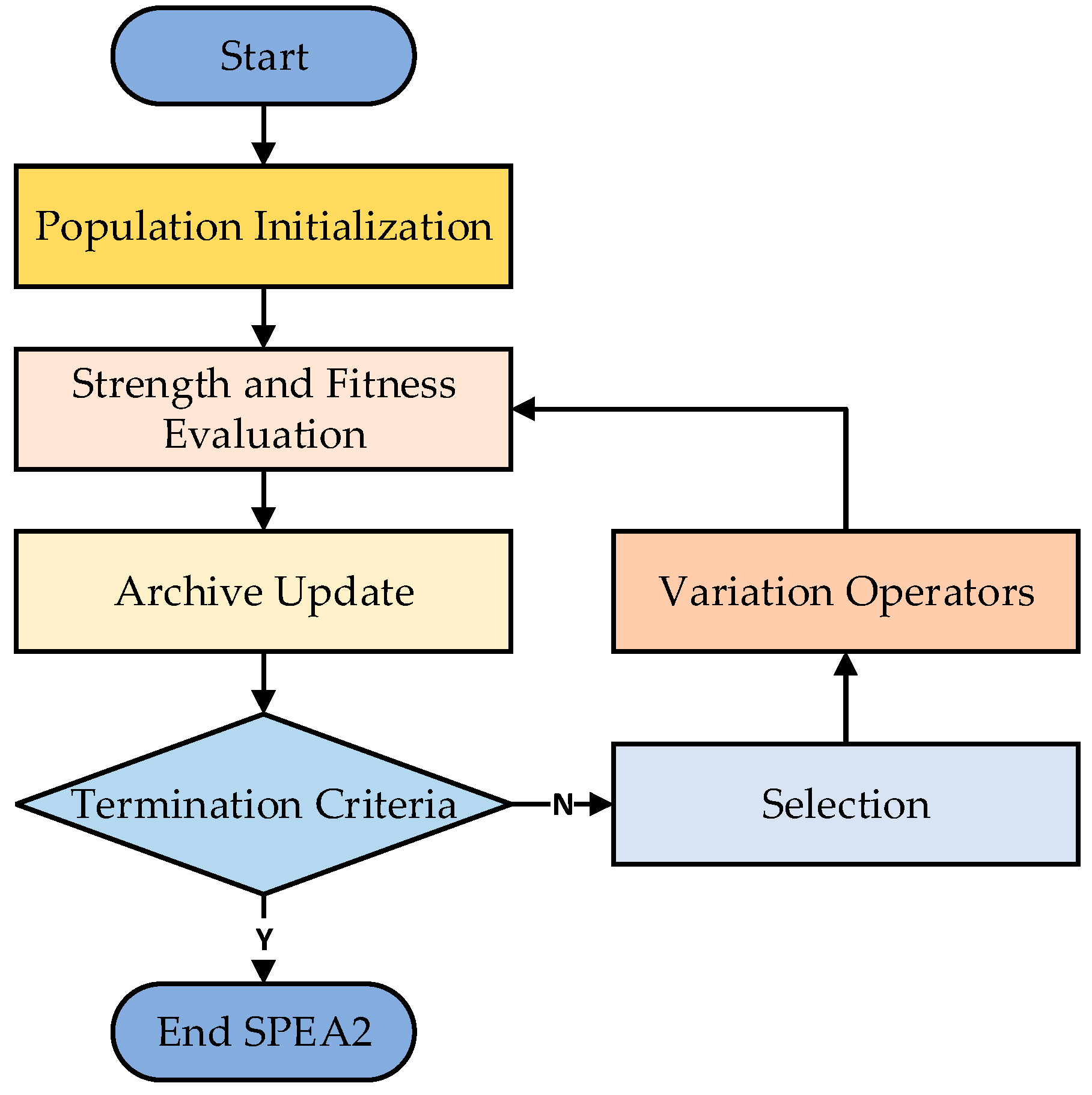
2.1. SPEA2 Algorithm

The Strength Pareto Evolutionary Algorithm 2 (SPEA2) [28] is a widely recognized and advanced multi-objective optimization algorithm. Its primary objective is to simulate natural selection to identify balanced solutions across multiple conflicting objectives. As a successor to the original SPEA algorithm [29], SPEA2 incorporates several enhancements, particularly in its handling of convergence (the ability to approach the Pareto-optimal front) and diversity (the distribution of solutions along the Pareto front). These improvements make SPEA2 a robust and effective tool for solving complex multi-objective optimization problems.
In SPEA2, the superiority of an individual solution is determined using “Pareto dominance”. Solution A is considered superior to Solution B if it is not worse than B on all objectives and better on at least one objective. To evaluate individual solutions effectively, SPEA2 introduces the concept of fitness, calculated based on two factors: individual strength and distance to other solutions. Specifically, the strength Ii is determined by the number of solutions that outperform individual i, as shown in the following equation:
I i = j P : f j f i
where P represents all the solutions in the current population and fj and fi represent the target values of the solutions and the target values of the solutions, respectively. Individual fitness Fi is evaluated by combining intensity and distance, and it is calculated as follows:
F i = I i + D i
where Di is the distance to the nearest solution in the elite pool, defined as follows:
D i = min j R   d ( f i , f j )
where R is an elite repository storing high-quality solutions and d represents the distance between two solutions. In the target space, the distance between two solutions can be obtained using the Euclidean distance formula as follows:
d ( f i , f j ) = k = 1 m f i ( k ) f j ( k ) 2
where m represents the number of objectives and fi(k) and fj(k) denote the values of solution i and solution j on the kth objective.
The SPEA2 algorithm operates iteratively. The flowchart in Figure 1 illustrates its key steps, which include the following:
  • Step 1: Population Initialization. An initial population P is randomly generated. The population size N is fixed, ensuring computational efficiency in fitness evaluation. An elite archive R is also initialized to store high-quality non-dominated solutions.
  • Step 2: Strength and Fitness Evaluation. For each solution in P and R, the dominance strength and fitness are computed as described above. The fitness values guide the selection process, balancing convergence to the Pareto front and diversity within the solution set.
  • Step 3: Archive Update. After fitness evaluation, the elite archive R is updated. Non-dominated solutions are added to R, while dominated solutions are removed. If R exceeds its maximum size, solutions are pruned using a truncation procedure based on proximity to other solutions.
  • Step 4: Selection. A mating pool is formed by selecting individuals based on their fitness values. Solutions with lower fitness values (better solutions) have a higher probability of being selected.
  • Step 5: Variation Operators. Genetic operators, such as crossover and mutation, are applied to the mating pool to generate a new population. These operators introduce variation, enabling exploration of the solution space.
  • Step 6: Termination. The process is repeated for a predefined number of generations or until a termination criterion (e.g., convergence of the population to the Pareto front) is met. The final elite archive R represents the set of non-dominated solutions that approximate the Pareto-optimal front.

2.2. MMBB Model

The following section introduces the architecture and advantages of the proposed MMBB model. The MMBB model is a lightweight convolutional neural network optimized for image classification tasks. It aims to enhance feature extraction and classification performance, as depicted in Figure 2. This model combines the efficient design of MobileNetV3 [30] with the Bottleneck Attention Module (BAM) [31] to achieve more accurate and faster diagnostic results across diverse application scenarios.
The network architecture includes an input layer, a feature extraction layer, a pooling layer, and a classification layer. The input layer processes single-channel image data, particularly suited for grayscale images. The feature extraction layer consists of a convolutional layer and an inverted residual block [32], which leverages depth separable convolutions to extract multi-level features, improving computational efficiency and reducing the number of parameters. The repeated use of the inverted residual block and BAMs is intended to enhance the depth and accuracy of feature extraction, while also improving the model’s computational efficiency and parameter utilization, ultimately optimizing the network’s performance in complex tasks.
Each inverted residual block contains three key components, and its structure is shown in Figure 3. First, a pointwise convolution is applied to expand the number of channels in the input features, thereby enhancing the expressive capacity of the network. This operation is represented as follows:
X hidden = C o n v 1 × 1 X i n
where Xhidden represents the output feature map, Xin represents the input feature map, and Conv1×1 represents a 1 × 1 convolution operation. Following this, a depth-separable convolution is performed, where each channel is processed individually, significantly reducing computational costs as follows:
X o u t = D e p t h w i s e C o n v 3 × 3 X h i d d e n
where Xout represents the output of the deep convolution with the number of channels preserving the number of input channels and DepthwiseConv3×3 represents the 3 × 3 convolution operation. Finally, the number of input channels is mapped back to the input channels by point-by-point convolution, which is calculated as follows:
Y = C o n v 1 × 1 ( X o u t )
where Y represents the final output feature map with the number of channels equal to the number of channels of Xout.
After each inverted residual block, the BAM is introduced to enhance the feature representation of the network. The BAM combines channel attention and spatial attention to adaptively adjust the importance of the feature map, and its structure is shown in Figure 4.
In the channel attention branch, global average pooling is applied to capture feature relationships across different channels. The pooling operation generates a channel vector, which is then processed through a multilayer perceptron (MLP), formulated as follows:
M c F = B N M L P A v g P o o l F   = B N W 1 W 0 A v g P o o l F + b 0 + b 1
where AvgPool denotes global average pooling and BN represents batch normalization. This process enhances the network’s ability to capture the most relevant channel-specific features.
The spatial attention branch complements the channel attention by focusing on specific regions of the feature map. Dimensionality reduction is achieved via a 1 × 1 convolution, followed by a 3 × 3 convolution to further enhance the receptive field. The spatial attention map is then calculated as follows:
M S ( F ) = B N f 1 × 1 3 f 3 × 3 2 f 3 × 3 1 f 1 × 1 0 F
where f denotes the convolution operation, the subscript of the convolution denotes the size of the convolution kernel, and the superscript of the convolution denotes the number of rounds. The channel and spatial attention maps are then combined and extended to the same dimension as follows:
M F = σ M c F + M s F
where σ is the Sigmoid function. The refined feature map F’ is finally obtained by integrating into the refined feature map by element level multiplication as follows:
F = F + F M F
where   denotes elementwise multiplication. This residual learning approach effectively facilitates gradient flow and enhances feature learning, resulting in a model that excels in both representation and performance.
The advantages of this network architecture lie in its high efficiency and adaptive feature extraction capabilities. By employing depthwise separable convolution and the BAM, the model reduces computational complexity and the number of parameters, while maintaining high accuracy. Moreover, the BAM allows the network to dynamically focus on critical features, improving overall performance and making it highly suitable for real-time fault diagnosis in distributed systems.

3. Overall Process

3.1. Problem Formulation

Suppose there are n faults in the system (composite faults exist) and the system is composed of n subsystems, each responsible for diagnosing one fault. The system has m sensors, denoted by x 1 , x 2 , ,   x m , respectively. Each subsystem selects a subset of sensors to be used for fault diagnosis. Let s i   i = 1 , 2 , 3 , , n represent the sensor selection vector for the i-th subsystem. It is an mmm-dimensional vector, where 0 indicates that the sensor is not selected and 1 indicates that the sensor is selected. The sensor selection can be expressed in matrix form as follows:
s 1 s 2 s 3 s n x 1 x 2 x 3 x m T = 1 0 1 1 1 1 0 1 1 0 1 0 0 0 1 1 x 1 x 2 x 3 x m = x 1 + x 3 + + x m x 1 + x 2 + + x m x 1 + x 3 + + x m 1 x 3 + + x m
After selecting the sensors, it is necessary to extract the data of the corresponding sensors from the dataset and then pass these data as inputs to the MMBB model for fault diagnosis, which is mathematically represented as follows:
d 1 d 2 d 3 d n m 1 m 2 m 3 m n = r e s u l t 1 r e s u l t 2 r e s u l t 3 r e s u l t n
where d i i = 1 , 2 , 3 , , n denotes a piece of data extracted from the dataset by each subsystem based on the selection of the sensor’s case set, m i i = 1 , 2 , 3 , , n denotes a function abstraction of the MMBB model, and r e s u l t i i = 1 , 2 , 3 , , n denotes the final diagnostic result of each subsystem.
The SPEA2 multi-objective optimization algorithm is employed to find an optimal solution for the sensor selection vector S, i.e., s 1 s 2 s 3 s n T , ensuring optimal diagnostic performance.

3.2. Definition of the Objective Function

Defining an effective objective function is a key component of the optimization process in distributed fault diagnosis systems. Traditional fault diagnosis systems are typically evaluated based on the accuracy of individual subsystems. However, this approach often fails to fully reflect the diagnostic performance of the entire system in a complex distributed environment. Because the accuracy rates of individual subsystems are independent and non-conflicting, using them as the sole objective function in the optimization process may lead to high problem dimensionality, increasing the complexity of finding an optimal solution.
To address this issue, this paper proposes a dual-objective optimization strategy that considers both the average accuracy of subsystems and the accuracy of the integrated system. This method not only evaluates the performance of individual subsystems but also ensures the diagnostic capability of the entire system by considering the integrated accuracy rate. The two objective functions are as follows:
F 1 = max 1 N i = 1 n A i ( s i ) = max 1 N i = 1 n j = 1 N a i j s i F 2 = max A o v e r a l l ( S ) = max 1 N i = 1 N a i S
where N denotes the number of test sets n denotes the number of subsystems. F1 and F2 denote two objective functions: F1 is used to describe the average accuracy of subsystems and F2 is used to describe the combined accuracy of the system. Ai(si) denotes the accuracy of the i-th subsystem and aij(si) denotes the accuracy of each test sample under sensor selection si of the i-th subsystem, where a correct value is 1 and an incorrect value is 0. Aoverall(S) denotes the combined accuracy of the system and ai(S) denotes the accuracy of each test sample under sensor selection S of the n subsystems. Aoverall(S) denotes the combined accuracy of the system and ai(S) denotes the accuracy of each test sample under the sensor selection S of the nth subsystem, and the specific calculation rules are presented in Table 1.
The accuracy calculation method mentioned above effectively evaluates the system’s fault detection capability, while the optimization of sensor combinations through the SPEA2 algorithm can significantly enhance the fault diagnosis accuracy.

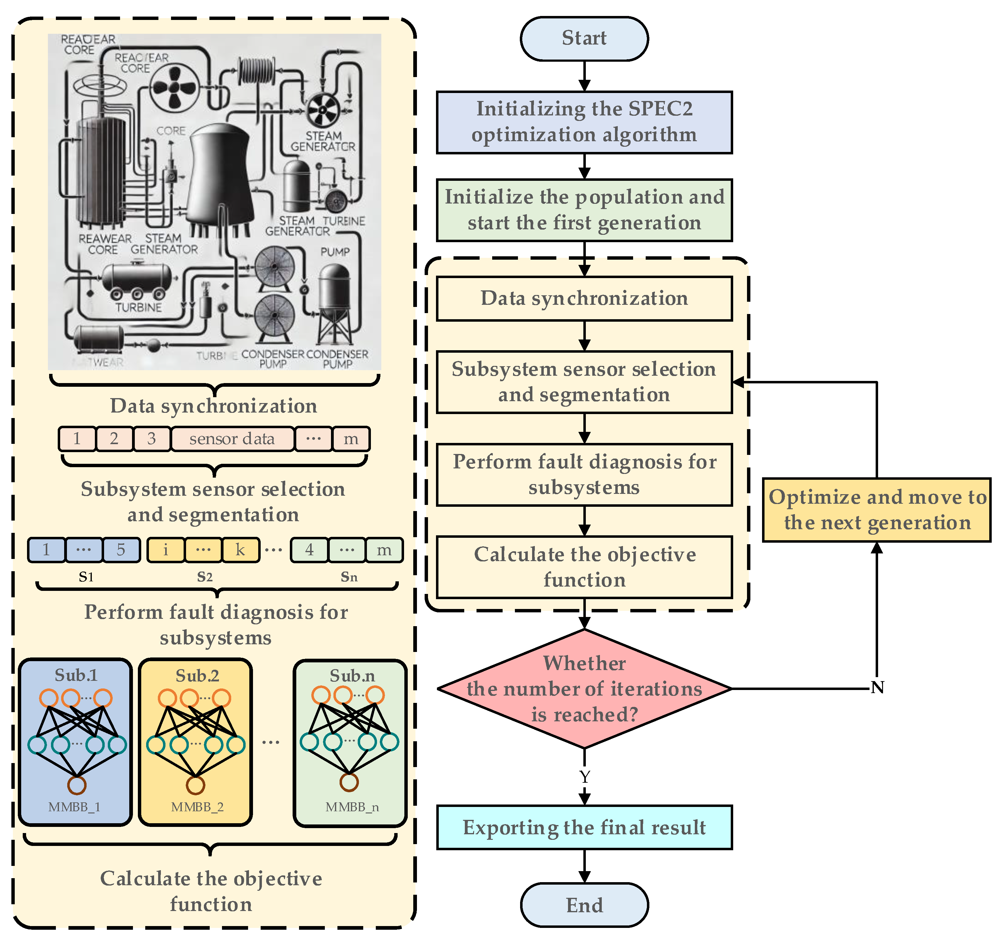
3.3. Optimization Process

The flowchart of the proposed methodology is illustrated in Figure 5 and can be summarized in the following steps:
  • Step 1. The SPEA2 algorithm is first executed for initialization, transforming the sensor optimization problem into a matrix-solving task.
  • Step 2. Prepare the elite solution and initialize the population to minimize the number of iteration rounds. Then, initiate the fault diagnosis using the first generation of sensor selections.
  • Step 3. Fault diagnosis is conducted using the selected sensors. The data are first synchronized to enable the calculation of combined accuracy. Then, the relevant sensor data are extracted and sent to different subsystems for fault diagnosis. Finally, the average accuracy of the subsystems and the combined accuracy of the system (the objective function) are computed.
  • Step 4. Check whether the maximum number of iterations has been reached. If not, optimize the sensor selection based on the diagnostic results from the previous round using the SPEA2 algorithm and proceed with a new round of fault diagnosis.
  • Step 5. Once the maximum number of iterations is reached, retrieve the elite individuals from the elite pool, which includes the selected sensors, the accuracy of each subsystem, and the combined accuracy of the system.

4. Case Study of the Reactor Coolant System

4.1. Experimental Dataset

This study primarily focuses on the Reactor Coolant System (RCS) of a nuclear power plant. The experiment investigates six common faults in the RCS, including a hot leg break in Loop 1, a cold leg break in Loop 1, a steam generator tube rupture, a pressurizer spray line leakage into the containment, a pressurizer safety valve stuck open, and a reactor pressure vessel vent line leakage. These faults are coded as RCS01, RCS03, RCS09, RCS13, RCS07, and RCS11, respectively, with their locations shown in Figure 6.
The experimental data were collected from a nuclear power plant simulation system, where data from 200 sensors in the RCS and related systems were gathered. After introducing the faults, the simulation system recorded sensor data at intervals of 0.5 s per entry into a database. The experiment involved the verification and analysis of data under various conditions, including single fault scenarios, as well as combinations of two to six faults, along with normal operating conditions, all based on six predefined faults. During the experiment, we collected data at 3000 time points for some potential faults that might occur. The details of the collected data are presented in Table 2.

4.2. Data Preprocessing

4.2.1. Removal of Low-Variance Data Using Variance Thresholding

Sensor features that have relatively low variance are removed by variance thresholding. Low variance features often lack sufficient information about the variation and are usually not helpful for model training. The variance is calculated using the following formula:
S 2 = 1 n i = 1 n x i x ¯ 2
where x ¯ represents the mean value of the sensor data. If the variance is less than 10, these sensor data are removed from the dataset.

4.2.2. Exclusion of Anomalies and Data Standardization

During the data preprocessing stage, outlier detection and data standardization are critical steps to ensure model validity. First, the rejection of anomalous data can be achieved through the standardization method by identifying and removing outliers that are far away from the data distribution, thus improving the data quality and the generalization ability of the model. To achieve this, the mean μ and standard deviation σ of the data are calculated, followed by transforming the data into a standard normal distribution using the Z-score formula as follows:
Z = X μ σ
Next, data points with Z-scores greater than 3 in absolute value are considered outliers, indicating that they lie more than three standard deviations from the mean. By eliminating these outliers, the quality of the data can be effectively improved. Finally, after removing the outliers, the dataset is standardized using the Z-score method.

4.2.3. Time Window Data Generation

The experiment comprises six subsystems, each responsible for diagnosing a specific fault. Each subsystem is associated with a distinct fault tag, labeled tag1, tag2, …, and tag6. During the experiment, the data processing is simplified by tagging each fault with a segment_id of the system to simplify the data processing process, and the data after tagging are shown in Figure 7a.
When training the model for each subsystem, a short time series of eight sensors needs to be extracted from the dataset, so the collected data must be sliced and diced by time windows. Each time window contains thirty time points, equivalent to 15 s of monitoring data, with a step size of five time points to minimize information loss, as shown in Figure 7b. The data can be used as the data source of the whole dataset, but the whole dataset is more than one time series.
However, the entire dataset comprises different faults across various time periods, requiring frequent screening of transitional data segments during model training and testing, which leads to significant time overhead. Meanwhile, due to the existence of overlapping windows, it is not easy to realize when dividing the training and testing sets, and the complexity of the algorithm will be high.
The time-series data, spanning 30 time points, are horizontally spliced, after which the segment_id is used to determine whether the data belong to the same fault period. If not, the data are discarded. This process is illustrated in Figure 7c. Finally, the data are organized and reordered, and the auxiliary label segment_id is removed.

4.3. Experimental Validation

In this study, the multi-objective optimization algorithm, SPEA2, was employed with the following settings: a population size of 30, 50 optimization generations, and 30 elite individuals based on expert knowledge were added to the initial population for the optimization process. The aforementioned MMBB model is defined as the evaluation model for the optimization algorithm.
During evaluation, the multivariate time series extracted by the multi-objective optimization algorithm is transformed into a 1 × 8 × 30 grayscale image for input. This input is passed through four feature extraction layers, each consisting of a combination of inverted residual blocks and BAM blocks. The output is then processed via mean pooling, followed by flattening, and finally passed through a classifier to produce the results, as detailed in Table 3.
This study determines the training parameters for the MMBB model through sensitivity analysis. The training data consist of sensor data selected based on expert knowledge, with the average accuracy of six subsystems used as the evaluation metric. Three learning rates (0.01, 0.001, 0.0001), three batch sizes (64, 128, 256), and two weight update algorithms, SGD (Stochastic Gradient Descent) and Adam (Adaptive Moment Estimation) were tested in a total of 18 experimental setups, as shown in Table 4. The results indicate that the best performance was achieved in the 17th experiment, where the MMBB model’s training parameters were as follows: a learning rate of 0.00001, a batch size of 128, 100 epochs, and an Adam optimizer.
Figure 8 presents the results of the MMBB model after sensor selection through the optimization algorithm, highlighting six elite solutions from the elite pool. The six elite solutions achieved an average subsystem accuracy of over 98.12%, while the overall system accuracy exceeded 94.66%, highlighting the model’s strong performance.
Among these, Elite Solution 6 is particularly notable, with an average subsystem accuracy of 98.73%. The accuracy rates of its six subsystems are 99.39%, 98.89%, 99.26%, 98.93%, 98.85%, and 97.13%, respectively, while the overall system accuracy reaches 95.22%. Figure 9 depicts the training process of Elite Solution 6. In this experiment, the six subsystems were trained synchronously over 100 epochs, exhibiting excellent classification capability and generalization performance. The training loss for all subsystems decreased significantly, while the test accuracy showed minimal fluctuations and a clear upward trend. This demonstrates that the model effectively learns and adapts to complex tasks.
Figure 10 displays the confusion matrix for the fault classification of the six subsystems. From the confusion matrix, we can observe the classification performance of each subsystem in diagnosing faults. The results indicate that each subsystem can classify faults with a high degree of accuracy.
Eight groups were established for this comparison experiment: a single-system optimization algorithm (PSO) combined with the MMBB model, LSTM neural network, CNN neural network, the SPEA2 optimization algorithm combined with both the LSTM and CNN neural network models, and the multi-objective optimization algorithm (DMOPSO) combined with the MMBB model, LSTM neural network, and CNN neural network. The parameters for the PSO and DMOPSO in the comparison experiments were set to 30 populations and 50 optimization generations, with the initial population added based on manual expertise. Both the LSTM and CNN networks were configured with four layers, consistent with the MMBB model.
Table 5 presents the results of optimizing subsystem and overall accuracy using the SPEA2 multi-objective optimization algorithm with different neural networks, as well as the results from the single-objective PSO and multi-objective DMOPSO. Among these, the LSTM and CNN neural networks exhibit lower accuracy in certain subsystems. However, when using the same optimization algorithm, the improved MMBB neural network demonstrates strong adaptability, with significantly higher subsystem and combined accuracy compared to the other neural network models.
In cases where the same neural network is used, sensor selection for fault diagnosis via the SPEA2 multi-objective optimization algorithm maintains subsystem accuracy at a level comparable to the single-objective PSO, but the combined accuracy is notably higher with SPEA2. When using the multi-objective optimization algorithm, DMOPSO, for optimization, both the subsystem accuracy and the overall accuracy are relatively low. Additionally, when the selected neural network results in low accuracy for some subsystems, the use of SPEA2 can significantly enhance the overall system accuracy.
Table 5 also presents the inference time and computational load for each experimental group, with the results obtained from an NVIDIA 3060 GPU platform (Colorful iGame GeForce RTX 3060 Ultra W OC 12G, manufactured by Colorful Technology Co., Ltd., Shenzhen, Guangdong, China). Regarding inference time, the MMBB model has a moderate duration of approximately 25 ms, while the CNN model exhibits the shortest inference time and the LSTM model the longest. However, all models meet the real-time requirements for distributed fault diagnosis. In terms of computational load, the LSTM model has the highest load, exceeding 30%, the MMBB model has a moderate load of approximately 26%, and the CNN model has the lowest load at approximately 18%. All models operate within reasonable limits.

5. Conclusions

(1)
Summary of Contributions
This study introduces an innovative distributed fault diagnosis method for nuclear power systems, integrating the SPEA2 multi-objective optimization algorithm with the MMBB neural network. The approach effectively addresses the challenges of multi-fault scenarios, dynamic feature selection, and system-wide optimization, achieving significant improvements in diagnostic accuracy while ensuring real-time performance. The experimental results demonstrated that the proposed method achieved an average subsystem accuracy of 98.73% and an overall system accuracy of 95.22%.
(2)
Key Advantages
  • The SPEA2 algorithm optimizes sensor feature selection dynamically, ensuring efficient resource utilization and enhanced fault detection capability.
  • The MMBB neural network demonstrates robust performance with superior classification accuracy across distributed subsystems.
  • The dynamic feedback mechanism between optimization and neural network training ensures adaptability and reliability in complex fault scenarios.
(3)
Limitations and Future Directions
  • Handling Missing Data and Sensor Failures. Future work will incorporate methods, like GANs, to address incomplete sensor data and enhance robustness against sensor faults in real-world applications.
  • Improving Model Interpretability. Future research will explore explainability techniques to make the model’s decision-making process more transparent for safety-critical applications.
  • Broader Comparisons. Expanding comparisons to include Bayesian networks and reinforcement learning techniques will provide a more comprehensive evaluation of the proposed approach.

Author Contributions

Conceptualization, Y.X., J.M. and J.Y.; Methodology, Y.X., J.M. and J.Y.; Software, Y.X.; Validation, Y.X.; Formal analysis, Y.X.; Resources, J.M.; Data curation, J.Y.; Writing—original draft, Y.X.; Writing—review & editing, J.M.; Visualization, Y.X.; Supervision, J.M.; Project administration, J.M.; Funding acquisition, J.M. All authors have read and agreed to the published version of the manuscript.

Funding

This research was funded by the National Natural Science Foundation of China, grant number 61973041.

Data Availability Statement

The datasets presented in this article are not readily available because they are subject to confidentiality agreements and contain sensitive information related to nuclear power plant operations. Requests to access the datasets should be directed to China Nuclear Power Engineering Co., Ltd.

Conflicts of Interest

Author Jinxiao Yuan was employed by the company China Nuclear Power Engineering Co., Ltd. The remaining authors declare that the research was conducted in the absence of any commercial or financial relationships that could be construed as a potential conflict of interest. The company had no role in the design of the study; in the collection, analyses, or interpretation of data; in the writing of the manuscript, or in the decision to publish the results.

References

  1. Qian, G.; Liu, J. Fault Diagnosis Based on Conditional Generative Adversarial Networks in Nuclear Power Plants. J. Electr. Eng. Technol. 2023, 176, 109267. [Google Scholar] [CrossRef]
  2. Zio, E. Advancing Nuclear Safety. Front. Nucl. Eng. 2023, 4, 75–90. [Google Scholar] [CrossRef]
  3. Chen, H.Y.; Wang, Y.C.; Huang, X.Y.; Tian, X.L. Accident Source Term and Radiological Consequences of a Small Modular Reactor. Nucl. Sci. Tech. 2023, 33, 101. [Google Scholar] [CrossRef]
  4. Peng, M.; Wang, H.; Yang, X.; Liu, Y.; Guo, L.; Li, W.; Jiang, N. Real-Time Simulations to Enhance Distributed on-Line Monitoring and Fault Detection in Pressurized Water Reactors. Ann. Nucl. Energy 2017, 109, 557–573. [Google Scholar] [CrossRef]
  5. Wu, G.; Duan, Z.; Yuan, D.; Yin, J.; Liu, C.; Ji, D. Distributed Fault Diagnosis Framework for Nuclear Power Plants. Front. Energy Res. 2021, 9, 665502. [Google Scholar] [CrossRef]
  6. Yang, G.; Su, J.; Du, S.; Duan, Q. Federated Transfer Learning-Based Distributed Fault Diagnosis Method for Rolling Bearings. Meas. Sci. Technol. 2024, 35, 126111. [Google Scholar] [CrossRef]
  7. Mousavi, A.; Mousavi, R.; Mousavi, Y.; Tavasoli, M.; Arab, A.; Fekih, A. Artificial Neural Networks-Based Fault Localization in Distributed Generation Integrated Networks Considering Fault Impedance. IEEE Access 2024, 12, 82880–82896. [Google Scholar] [CrossRef]
  8. Castelletti, F.; Niro, F.; Denti, M.; Tessera, D.; Pozzi, A. Bayesian Learning of Causal Networks for Unsupervised Fault Diagnosis in Distributed Energy Systems. IEEE Access 2024, 12, 61185–61197. [Google Scholar] [CrossRef]
  9. Rajabioun, R.; Afshar, M.; Atan, O.; Mete, M.; Akin, B. Classification of Distributed Bearing Faults Using a Novel Sensory Board and Deep Learning Networks With Hybrid Inputs. IEEE Trans. Energy Convers. 2024, 39, 963–973. [Google Scholar] [CrossRef]
  10. Feng, B.; Zhou, Q.; Xing, J.; Yang, Q. Distributed Chaotic Bat Algorithm for Sensor Fault Diagnosis in AHUs Based on a Decentralized Structure. J. Build. Eng. 2024, 95, 110031. [Google Scholar] [CrossRef]
  11. Peng, H.; Mao, Z.; Jiang, B.; Cheng, Y. Multiscale Spatial-Temporal Bayesian Graph Conv-Transformer-Based Distributed Fault Diagnosis for UAVs Swarm System. IEEE Trans. Aerosp. Electron. Syst. 2024, 60, 6894–6909. [Google Scholar] [CrossRef]
  12. Ding, X.; Liao, X.; Cui, W.; Meng, X.; Liu, R.; Ye, Q.; Li, D. A Deep Reinforcement Learning Optimization Method Considering Network Node Failures. Energies 2024, 17, 4471. [Google Scholar] [CrossRef]
  13. Li, Q.; Wang, Y.; Dong, J.; Zhang, C.; Peng, K. Multi-Node Knowledge Graph Assisted Distributed Fault Detection for Large-Scale Industrial Processes Based on Graph Attention Network and Bidirectional LSTMs. Neural Netw. 2024, 173, 106210. [Google Scholar] [CrossRef]
  14. Ren, C.; Li, H.; Lei, J.; Liu, J.; Li, W.; Gao, K.; Huang, G.; Yang, X.; Yu, T. A CNN-LSTM-Based Model to Fault Diagnosis for CPR1000. Nucl. Technol. 2023, 209, 1365–1372. [Google Scholar] [CrossRef]
  15. Zhang, C.; Chen, P.; Jiang, F.; Xie, J.; Yu, T. Fault Diagnosis of Nuclear Power Plant Based on Sparrow Search Algorithm Optimized CNN-LSTM Neural Network. Energies 2023, 16, 2934. [Google Scholar] [CrossRef]
  16. Xu, Y.; Cai, Y.; Song, L. Latent Fault Detection and Diagnosis for Control Rods Drive Mechanisms in Nuclear Power Reactor Based on GRU-AE. IEEE Sens. J. 2023, 23, 6018–6026. [Google Scholar] [CrossRef]
  17. Jin, I.J.; Lim, D.Y.; Bang, I.C. Deep-Learning-Based System-Scale Diagnosis of a Nuclear Power Plant with Multiple Infrared Cameras. Nucl. Eng. Technol. 2023, 55, 493–505. [Google Scholar] [CrossRef]
  18. Lin, W.; Miao, X.; Chen, J.; Ye, M.; Xu, Y.; Liu, X.; Jiang, H.; Lu, Y. Fault Detection and Isolation for Multi-Type Sensors in Nuclear Power Plants via a Knowledge-Guided Spatial-Temporal Model. Knowl.-Based Syst. 2024, 300, 112182. [Google Scholar] [CrossRef]
  19. Huang, X.; Xia, H.; Liu, Y.; Miyombo, M.E. Improved Fault Diagnosis Method of Electric Gate Valve in Nuclear Power Plant. Ann. Nucl. Energy 2023, 194, 109996. [Google Scholar] [CrossRef]
  20. Dai, H.; Liu, X.; Zhao, J.; Wang, Z.; Liu, Y.; Zhu, G.; Li, B.; Abbasi, H.N.; Wang, X. Modeling and Diagnosis of Water Quality Parameters in Wastewater Treatment Process Based on Improved Particle Swarm Optimization and Self-Organizing Neural Network. J. Environ. Chem. Eng. 2024, 12, 113142. [Google Scholar] [CrossRef]
  21. Chang, X.; Yang, S.; Li, S.; Gu, X. Rolling Element Bearing Fault Diagnosis Based on Multi-Objective Optimized Deep Auto-Encoder. Meas. Sci. Technol. 2024, 35, 096007. [Google Scholar] [CrossRef]
  22. Wang, Z.-C.; Wang, S.-C.; Li, D.; Cao, Z.-W.; He, Y.-L. An Intelligent Fault Detection and Diagnosis Model for Refrigeration Systems with a Comprehensive Feature Selection Method. Int. J. Refrig. 2024, 160, 28–39. [Google Scholar] [CrossRef]
  23. Aghababaeyan, Z.; Abdellatif, M.; Dadkhah, M.; Briand, L. DeepGD: A Multi-Objective Black-Box Test Selection Approach for Deep Neural Networks. ACM Trans. Softw. Eng. Methodol. 2024, 33, 158. [Google Scholar] [CrossRef]
  24. Ji, C.; Zhang, C.; Suo, L.; Liu, Q.; Peng, T. Swarm Intelligence Based Deep Learning Model via Improved Whale Optimization Algorithm and Bi-Directional Long Short-Term Memory for Fault Diagnosis of Chemical Processes. ISA Trans. 2024, 147, 227–238. [Google Scholar] [CrossRef]
  25. Yang, P.; Wang, T.; Yang, H.; Meng, C.; Zhang, H.; Cheng, L. The Performance of Electronic Current Transformer Fault Diagnosis Model: Using an Improved Whale Optimization Algorithm and RBF Neural Network. Electronics 2023, 12, 1066. [Google Scholar] [CrossRef]
  26. Zhao, H.; Liu, M.; Sun, Y.; Chen, Z.; Duan, G.; Cao, X. Automated Design of Fault Diagnosis CNN Network for Satellite Attitude Control Systems. IEEE T. Cybern. 2024, 54, 4028–4038. [Google Scholar] [CrossRef]
  27. Wang, M.-H.; Chan, F.-C.; Lu, S.-D. Using a One-Dimensional Convolutional Neural Network with Taguchi Parametric Optimization for a Permanent-Magnet Synchronous Motor Fault-Diagnosis System. Processes 2024, 12, 860. [Google Scholar] [CrossRef]
  28. Zitzler, E.; Laumanns, M.; Thiele, L. SPEA2: Improving the Strength Pareto Evolutionary Algorithm; ETH Zurich: Zürich, Switzerland, 2001; p. 21. [Google Scholar] [CrossRef]
  29. Zitzler, E.; Thiele, L. Multiobjective Evolutionary Algorithms: A Comparative Case Study and the Strength Pareto Approach. IEEE Trans. Evol. Computat. 1999, 3, 257–271. [Google Scholar] [CrossRef]
  30. Howard, A.; Sandler, M.; Chu, G.; Chen, L.-C.; Chen, B.; Tan, M.; Wang, W.; Zhu, Y.; Pang, R.; Vasudevan, V.; et al. Searching for MobileNetV3. arXiv 2019, arXiv:1905.02244. [Google Scholar] [CrossRef]
  31. Park, J.; Woo, S.; Lee, J.-Y.; Kweon, I.S. BAM: Bottleneck Attention Module. arXiv 2018, arXiv:1807.06514. [Google Scholar] [CrossRef]
  32. Sandler, M.; Howard, A.; Zhu, M.; Zhmoginov, A.; Chen, L.-C. MobileNetV2: Inverted Residuals and Linear Bottlenecks. arXiv 2019, arXiv:1801.04381. [Google Scholar] [CrossRef]
Figure 1. Flowchart of the SPEA2 algorithm.
Processes 12 02620 g001
Figure 2. Architecture of the MMBB model.
Processes 12 02620 g002
Figure 3. Structure of the inverted residual block.
Processes 12 02620 g003
Figure 4. Structure of the BAM module.
Processes 12 02620 g004
Figure 5. Flowchart of the structure of the optimization process.
Processes 12 02620 g005
Figure 6. The structure of the Reactor Coolant System and the locations of the faults.
Processes 12 02620 g006
Figure 7. (a) Add tags and segment_id to fault data according to subsystems. (b) Add time windows to fault data. (c) Splice data horizontally and remove transition sequences.
Processes 12 02620 g007
Figure 8. Subsystem accuracy and overall accuracy from the SPEA2-MMBB.
Processes 12 02620 g008
Figure 9. (a) Test set accuracy over epochs for the sixth elite individual. (b) Training set loss over epochs for the sixth elite individual.
Processes 12 02620 g009
Figure 10. (a) Confusion matrix of Subsystem 1. (b) Confusion matrix of Subsystem 2. (c) Confusion matrix of Subsystem 3. (d) Confusion matrix of Subsystem 4. (e) Confusion matrix of Subsystem 5. (f) Confusion matrix of Subsystem 6.
Processes 12 02620 g010
Table 1. The specific calculation rules of ai(S).
Fault Diagnosis Situation a i S
No missed detections and no misdiagnoses1
No missed detections, and only one non-faulty subsystem is misdiagnosed as faulty0.5
No missed detections, and only two non-faulty subsystems are misdiagnosed as faulty0.2
There is at least one missed diagnosis, or three or more non-faulty subsystems are misdiagnosed as faulty0
Table 2. Fault description and dataset composition for the RCS-distributed fault diagnosis system.
Type of FaultsDescriptionTime Points
NormalFull power3000
Single fault A hot leg break in Loop 1 (RCS01)3000
A cold leg break in Loop 1 (RCS03)3000
A steam generator tube rupture (RCS09)3000
A pressurizer spray line leakage into the containment (RCS13)3000
A pressurizer safety valve stuck open (RCS07)3000
A reactor pressure vessel vent line leakage (RCS11)3000
Combinations of two faultsRCS01 + RCS033000
RCS03 + RCS073000
RCS03 + RCS093000
RCS03 + RCS133000
RCS07 + RCS113000
RCS09 + RCS113000
Combinations of three faultsRCS01 + RCS03 + RCS073000
RCS01 + RCS03 + RCS113000
RCS01 + RCS07 + RCS113000
RCS03 + RCS09 + RCS133000
RCS03 + RCS13 + RCS073000
RCS09 + RCS07 + RCS113000
Combinations of four faultsRCS01 + RCS03 + RCS09 + RCS113000
RCS01 + RCS03 + RCS09 + RCS133000
RCS01 + RCS09 + RCS07 + RCS113000
RCS01 + RCS09 + RCS13 + RCS073000
RCS03 + RCS13 + RCS07 + RCS113000
RCS09 + RCS13 + RCS07 + RCS113000
Combinations of five faultsRCS01 + RCS03 + RCS09 + RCS13 + RCS073000
RCS01 + RCS03 + RCS13 + RCS07 + RCS113000
RCS01 + RCS09 + RCS13 + RCS07 + RCS113000
RCS03 + RCS09 + RCS13 + RCS07 + RCS113000
Combinations of six faultsRCS01 + RCS03 + RCS09 + RCS13 + RCS07 + RCS113000
Table 3. Parameter settings for each layer of the MMBB model.
Type of LayerInput Size and Output SizeParameter Description
Conv2d + BatchNorm2d + ReLU(batch_size, 1, 8, 30)
(batch_size, 16, 4, 15)
Conv2d: 16 filters, 3 × 3 kernel, stride = 2, padding = 1
Inverted Residual Block 1(batch_size, 16, 4, 15)
(batch_size, 24, 2, 8)
Expansion ratio: 4
Stride: 2
BAM Block 1(batch_size, 24, 2, 8)
(batch_size, 24, 2, 8)
Reduction ratio: 16
Dilation value: 4
Inverted Residual Block 2(batch_size, 24, 2, 8)
(batch_size, 32, 1, 4)
Expansion ratio: 4
Stride: 2
BAM Block 2(batch_size, 32, 1, 4)
(batch_size, 32, 1, 4)
Reduction ratio: 16
Dilation value: 4
Inverted Residual Block 3(batch_size, 64, 1, 2)
(batch_size, 64, 1, 2)
Expansion ratio: 4
Stride: 2
BAM Block 3(batch_size, 64, 1, 2)
(batch_size, 64, 1, 2)
Reduction ratio: 16
Dilation value: 4
Inverted Residual Block 4(batch_size, 96, 1, 2)
(batch_size, 96, 1, 2)
Expansion ratio: 4
Stride: 2
BAM Block 4(batch_size, 96, 1, 2)
(batch_size, 96, 1, 2)
Reduction ratio: 16
Dilation value: 4
AdaptiveAvgPool2d(batch_size, 96, 1, 2)
(batch_size, 96, 1, 1)
--
Flatten(batch_size, 96, 1, 1)
(batch_size, 96)
--
Linear (Classifier)(batch_size, 96)
(batch_size, num_classes)
Fully connected layer
Output size: 2
Table 4. The results of sensitivity experiments conducted with different parameters.
Experimental GroupLearning
Rate
Batch
Size
EpochOptimizer
for Weight Updates
Average
Accuracy
Comparison 10.00164100SGD85.97%
Comparison 20.001128100SGD87.26%
Comparison 30.001256100SGD85.92%
Comparison 40.000164100SGD87.94%
Comparison 50.0001128100SGD90.31%
Comparison 60.0001256100SGD88.11%
Comparison 70.0000164100SGD93.62%
Comparison 80.00001128100SGD94.33%
Comparison 90.00001256100SGD93.82%
Comparison 100.00164100Adam86.63%
Comparison 110.001128100Adam88.51%
Comparison 120.001256100Adam87.33%
Comparison 130.000164100Adam91.22%
Comparison 140.0001128100Adam92.34%
Comparison 150.0001256100Adam91.35%
Comparison 160.0000164100Adam94.22%
Comparison 170.00001128100Adam95.78%
Comparison 180.00001256100Adam93.46%
Table 5. Comparison of subsystem accuracy, overall accuracy, inference time, and computational load using different optimization algorithms and neural networks.
Experimental GroupOptimization
Algorithm
Neural
Network
Subsystem
Accuracy
Overall
Accuracy
Inference
Time
Computational Load
Basic GroupSPEA2MMBB99.39% 98.89% 99.26% 98.93% 98.85% 97.13%95.22%25 ms26%
Comparison 1LSTM97.56% 98.21% 98.81% 96.91% 97.48% 92.65%89.04%36 ms33%
Comparison 2CNN98.31% 98.45% 97.76% 98.93% 96.21% 95.32%91.13%18 ms18%
Comparison 3DMOPSOMMBB95.34% 94.76% 98.25% 98.62% 94.43% 92.13%90.22%25 ms25%
Comparison 4LSTM97.56% 98.38% 98.81% 95.91% 97.73% 87.65%83.04%34 ms33%
Comparison 5CNN93.46% 95.53% 93.76% 92.26% 93.35% 87.34%79.13%18 ms18%
Comparison 6PSOMMBB99.46% 98.83% 99.57% 98.70% 98.94% 97.41%93.74%26 ms26%
Comparison 7LSTM97.86% 98.33% 98.06% 97.12% 97.26% 92.42%84.43%33 ms32%
Comparison 8CNN98.36% 98.24% 97.92% 98.89% 96.35% 95.49%86.39%19 ms18%
Disclaimer/Publisher’s Note: The statements, opinions and data contained in all publications are solely those of the individual author(s) and contributor(s) and not of MDPI and/or the editor(s). MDPI and/or the editor(s) disclaim responsibility for any injury to people or property resulting from any ideas, methods, instructions or products referred to in the content.

