Investigation of Influence of High Pressure on the Design of Deep-Water Horizontal Separator and Droplet Evolution

Abstract

Under deep-water high-pressure conditions, the multiphase flow characteristics within separators show significant differences compared to conventional separators. When designing subsea separators, it is crucial to consider the impact of pressure to ensure that the design meets the separation objectives while remaining cost effective. This study enhances the theoretical foundations of subsea separator design by analyzing droplet motion behaviors under high pressure and incorporating these influences into a rational design framework. A horizontal separator was designed and integrated into a laboratory-scale separation system for experimental validation. Through the comprehensive testing of separation efficiencies and process dynamics, it was found that increased pressures resulted in a decrease in oil droplet sizes; at pressures exceeding 6 MPa, droplet diameters were observed to drop below 100 μm. This reduction in droplet size extends the required separation time, necessitating larger separator dimensions at higher operational pressures to maintain adequate separation quality. Numerical simulations complement experimental findings by clarifying the underlying separation mechanisms under high-pressure conditions and offering design recommendations for separators deployed in deep-water environments.

1. Introduction

Global oil and gas reserves and production are increasing. The focus of oil and gas exploration has gradually shifted toward deep water. Deep-water oil and gas exploration commenced in the late 1970s [1]. It is projected that up to 40% of future oil and gas reserves will be found in deep-water regions. Since the beginning of the 21st century, over half of the major oil and gas discoveries have occurred in deep-water regions. Notably, over 70% of the top 10 annual oil and gas discoveries were made in deep-water regions from 2012 to 2014, indicating significant potential for the development of deep-water resources [2,3,4].

As the ongoing development of oilfields continues, the water content of the produced fluid in an increasing number of oilfields has also increased. A critical challenge faced in modern offshore hydrocarbon extraction relates to the excessively high water content of the produced fluids, highlighting the need for advanced treatment methodologies aimed at oil–gas–water separation [5,6,7]. According to the statistics of relevant departments, the number of oil wells with a water content exceeding 80% has surpassed 40,000 and continues to grow rapidly [8].

Gravity separation is one of the most common methods employed in multiphase flow handling, particularly in the oil and gas sectors [9,10]. Its widespread use can be largely attributed to several inherent characteristics, such as simplicity and efficiency. The fundamental principle of gravity separation relies on the differential density of the components within mixtures, effectively separating immiscible substances without the need for external mechanical force. The effectiveness of gravity-based separation techniques has been thoroughly examined through both theoretical modeling and empirical investigation, providing insights into their operational parameters and limitations. Researchers have meticulously analyzed the influence of key variables, including temperature, pressure, and phase composition, on separation efficiency, optimizing the design and implementation of gravity separators [11,12,13].

In deep-water oil and gas production, the direct transportation of unprocessed fluids from the seabed to surface installations incurs substantial energy losses. The unnecessary conveyance of large volumes of water inflates the energy requirements for lifting operations, leading to heightened operational costs. Concurrently, this practice imposes additional stress on offshore processing infrastructure, demanding greater capacities for separation, treatment, and handling functions aboard the platforms. Such demands contradict the contemporary drive for compact and lightweight platform architectures aimed at optimizing space and reducing costs. Consequently, dedicated research efforts are not only necessary but also critically important [14,15]. In contrast to terrestrial separation processes, subsea separation technologies face a unique set of challenges and complexities that are fundamentally shaped by the ambient conditions prevalent in deep oceanic environments. The high-pressure regime and colder temperatures present at depth significantly alter the physical properties of the multiphase flow being processed, affecting factors such as viscosity, solubility, and phase behavior. Consequently, the design and operational parameters of subsea separators require meticulous calibrations. This necessitates a thorough understanding of fluid mechanics and phase equilibrium theory tailored specifically for deep-water settings.

The design of separators is constrained by nonlinear fluid dynamics, which poses significant challenges and represents an important issue in oil and gas development. Numerous studies have discussed foundational design methods for separators [16,17,18,19,20,21,22,23,24]. These design processes for conventional separators typically assume that the separator functions as a semi-full liquid container without liquid level control. They have been simplified due to industrial design requirements, often relying on empirical rules or semi-empirical methods. This has led to significant limitations in practical applications, which is primarily due to the lack of consideration of broader application environments. The design methods provided by API [25] are mainly based on the handling capacity of each phase in the oil and gas fields and the gas–liquid volume ratio of the separator, calculating the flow rates of gas and liquid phases, and subsequently determining the separator size. Monnery and Svrcek [18,19] clarified the design process of separators; however, the design methods still heavily depend on empirical rules, necessitating the selection of appropriate parameters from extensive tables. The choice of parameters directly influences the size of the separator. Arnold and Stewart [16,17], among others, have conducted thorough research on the calculations of the gap length and diameter of separators, summarizing design methods and calculation processes.

One of the pioneering subsea separation systems is the Subsea Separation Boosting and Injection (SSBI), deployed in the Tordis field, which is located approximately 200 m beneath sea level [26]. The SSBI serves as the world’s first subsea processing facility. The purpose of the Tordis SSBI is to separate water and hydrocarbons from the existing production fluid and to boost production. The Marlim field has adopted a pipeline-based separation solution that is particularly suited to deep-water operations. The separation pipeline in Marlim extends up to 60 m [27,28]. Saipem’s Spoolsep solution represents another innovative approach to subsea separation [29]. Spoolsep addresses the limitations imposed by a one-pipe solution, improving separation efficiency and capacity. Additionally, the integration of membrane technology and chemical additives is commonly employed in subsea separation processes.

The design theory of separators primarily references droplet motion theory in multiphase flows. Since horizontal separators rely mainly on gravity for separation, it is essential to focus on the motion of the droplets in the direction of gravity. The ratio of the time required for dispersed phase droplets to move vertically to the time required to move horizontally serves as an important reference standard for determining the separation efficiency of gravity separators. The effective space of the separator is simplified to a rectangular box with lengths L, B, and H. The horizontal movement time of the dispersed phase droplets is t₁ and the vertical movement time is t₂. Under a constant handling capacity Q, t₁ is a function of L, B, and H, whereas t₂ is related to H. The ratio of t₁ to t₂ is only related to the flow field parameters L and B, and it is dependent on the densities of each phase and the droplet size but independent of H. This is known as “shallow pool theory”, which is commonly used to optimize the structure in separator design, such as adding inclined plates and other aggregation structures.

Currently, research findings on the design theory of deep-water separators are relatively limited, and previous studies have primarily depended on the empirical selection of design parameters, lacking relevant theoretical support. The design of deep-water high-pressure separators must be examined from the perspective of dispersed phase droplet motion, conducting thorough studies on the effects of high pressure, and subsequently applying this knowledge to the design of separators.

To assess the separation performance of deep-water horizontal separators, we developed an experimental prototype and performed tests on the oil–water separation process, documenting the pressure and phase interface changes within the separator, measuring the oil content in the separated water solution, and quantitatively analyzing the separator’s separation performance. Additionally, numerical simulations were carried out to predict the changes in droplet size under high pressure, providing insights into separator performance in such conditions.

2. Droplet Behavior in the Separation Process and Separator Design

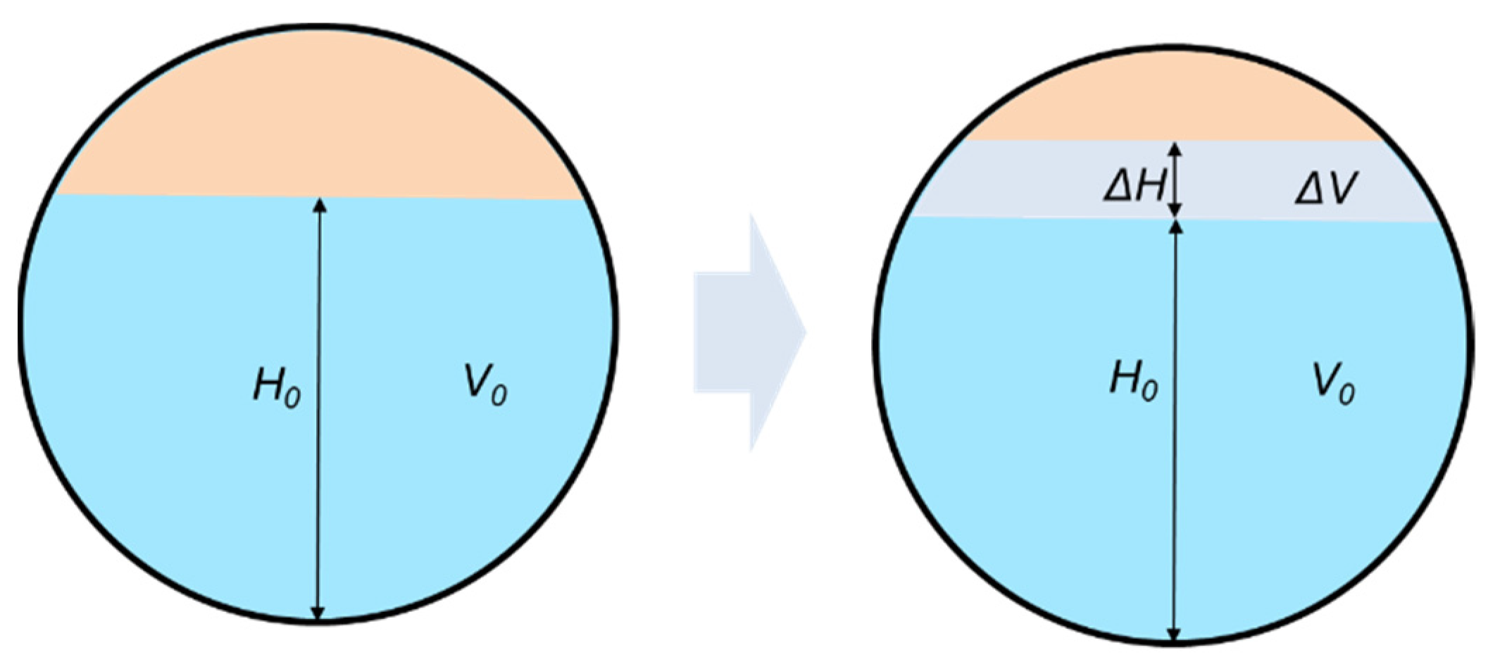
2.1. Behavior of Dispersed Phase Droplets During Phase Separation

The fundamental principle of two-phase gravity separation is bases on droplet settling theory, which involves examining the forces and motion processes acting on droplets in the continuous phase under the influence of gravity. By determining the final velocity component of droplets in the vertical direction based on the forces acting on the oil droplets in the continuous phase, the settling time of the droplets can be calculated. This time parameter is then compared with the capacity design calculation time of the separator to ascertain its dimensions. The ability of dispersed phase droplets to achieve gravity separation relies on the density difference between the two phases; thus, the sign of the density difference dictates the movement direction of the dispersed phase droplets. For analytical purposes, this paper refers to the vertical movement of droplets as settling motion. According to Archimedes’ principle, the relative buoyancy acting on dispersed phase droplets is

$$F_B={\displaystyle \frac{{\rho }_c\pi d_m^{3}g}{6}}-{\displaystyle \frac{{\rho }_o\pi d_m^{3}g}{6}}={\displaystyle \frac{({\rho }_c-{\rho }_o)\pi d_m^{3}g}{6}},$$

(1)

where ρ_c is the density of the continuous phase (in kg/m³), ρ_o is the density of the droplet (in kg/m³), d_m is the droplet size (in μm), and g is the acceleration due to gravity (m²/s).

The drag force is given by

$$F_D={\displaystyle \frac{C_D{A}_o{\rho }_c{V}^2}{2}}={\displaystyle \frac{C_D{\rho }_c\pi d_m^2{V}^2}{8}},$$

(2)

where C_D is the drag coefficient, A_o is the projected area of the droplet in the vertical direction (in m²), and V is the vertical velocity (in m/s).

According to the force balance condition, the velocity of the oil droplet moving at a constant velocity is

$$V=\sqrt{{\displaystyle \frac{4({\rho }_c-{\rho }_o)g{d}_m}{3C_D{\rho }_c}}},$$

(3)

In some studies [18,24], the separation velocity formula is transformed into

$$V=K\sqrt{{\displaystyle \frac{{\rho }_c-{\rho }_o}{{\rho }_c}}},$$

(4)

where

$$K=\sqrt{{\displaystyle \frac{4g{d}_m}{3C_D}}},$$

(5)

Svrcek et al. [18] have summarized the selection of K values based on engineering manuals and extensive field experience. If a mist eliminator is installed in the separator, the selection of K values refers to

Table 1. Selection of K value.

Operating Pressure, P (psia)	Calculation of K
1 ≤ P < 15	K = 0.1821 + 0.0029P + 0.046ln(P)
15 ≤ P < 40	K = 0.35
40 ≤ P ≤ 5500	K = 0.43 − 0.023ln(P)

. For horizontal separators, the drag coefficient C_D is calculated according to Equation (6).

$$C_D={\displaystyle \frac{5.0074}{\ln (x)}}+{\displaystyle \frac{40.927}{\sqrt{x}}}+{\displaystyle \frac{44.07}{x}},$$

(6)

Equation (3) illustrates that the droplet motion velocity is influenced by the density of the continuous phase, the density of the droplet, the droplet size, and the drag coefficient. Conventional separation often utilizes Stokes’ law to determine the drag coefficient, which is a widely used calculation method in engineering. At low Reynolds numbers, the predicted drag coefficient closely aligns with the experimental values, and the calculation formula is

$$C_D={\displaystyle \frac{24}{Re}},$$

(7)

However, in the design parameters of separators, the flow within the separator typically results in Reynolds numbers ranging from 1 to 100. Laleh et al. [24] have employed a more accurate Abraham formula for calculating the drag coefficient, which is given by

$$C_D=0.28{(1+{\displaystyle \frac{9.06}{\sqrt{Re}}})}^2,$$

(8)

The movement of oil droplets at a constant velocity constitutes the separation process itself. Solving Equation (3) indicates that the drag coefficient is influenced by velocity, while the physical parameters of the continuous phase and oil droplets, such as density and viscosity, remain constant. Once pressure and temperature are determined, the calculation of separation velocity solely on droplet size, as shown in the following equation:

$$\begin{array}{cc}\hfill C_D& =0.28{(1+9.06\cdot {10}^3\sqrt{{\displaystyle \frac{{\mu }_c}{{\rho }_c{d}_m{V}_{sep}}}})}^2\hfill \\ & ={\displaystyle \frac{4\cdot {10}^{-6}g{d}_m({\rho }_c-{\rho }_o)}{3{\rho }_c{V}^2}}\hfill \end{array},$$

(9)

where μ_c is the viscosity of the continuous phase (in Pa·s), V_sep is the separation velocity of the dispersed phase (in m/s), ρ_c is the density of the continuous phase (in kg/m³), ρ_o is the density of the droplet (in kg/m³) and d_m is the droplet size (in μm).

Since the drag coefficient derived from Equation (9) is influenced by the droplet settling velocity, the final settling velocity calculation for fixed droplet sizes should be performed iteratively. The larger the droplet size, the greater the drag force it encounters, resulting in a higher final settling velocity and a shorter separation time. Consequently, the size of dispersed phase droplets directly affects the design dimensions of the separator.

2.2. Separator Design Process

API SPEC 12J [25] has established a corresponding relationship table for the rated working pressure and dimensions of separators. In addition to selecting dimensions based on pressure, API also provides specifications for the calculation process based on the gas handling capacity, oil phase handling capacity, operating temperature, operating pressure, densities of each phase, and type of separator. This calculation process initially makes fundamental assumptions regarding the length of the separator and the volume of liquid, converting apparent velocity based on K values, and subsequently calculating the flow area based on actual flow rates to determine the separator diameter based on area ratios. The liquid handling capacity of two-phase separators primarily relies on the liquid residence time. Basic parameters for the liquid residence time, as provided by API, are displayed in

Table 2. Residence time for different oils.

API Gravity	Residence Time (min)
>35°	1
20°~30°	1~2
10°~20°	2~4

. This calculation method does not consider numerous factors, such as the specific process of liquid settling and the viscosity of the continuous phase. Furthermore, in many engineering designs, the cross-sectional area ratio and residence time cannot directly utilize empirical parameters due to the influence of physical parameters and working conditions in oil and gas fields.

In separator design, a commonly used method is to establish a capacity balance equation based on the relationship between the capacity and flow of each phase within the separator. The following capacity balance equation for the gas phase in the separator is formulated under the operating temperature and pressure [23]:

$$D{L}_{eff}=0.345\left({\displaystyle \frac{1-{\beta }_l}{1-{\alpha }_l}}\right)\left({\displaystyle \frac{TZ{Q}_g}{P}}\right){\left[\left({\displaystyle \frac{{\rho }_g}{{\rho }_l-{\rho }_g}}\right){\displaystyle \frac{C_D}{d_l}}\right]}^{1/2},$$

(10)

where α_l is the ratio of the liquid phase cross-sectional area to the separator cross-sectional area, β_l is the ratio of liquid level height to the separator diameter, L_eff is the effective length of the separator (in m), T is the operating temperature (in K), Qg is the gas phase flow rate (m³/s), P is the operating pressure (in kPa), Z represents gas compressibility, d_l is the droplet size (in μm), D is the inner separator diameter (in m), and ρ_g and ρ_l are the densities of the gas and liquid phases (in kg/m³), respectively.

The calculation of C_D refers to Equation (6), and the calculation of coefficient x is given by

$$x={\displaystyle \frac{3.35\times {10}^{-9}{\rho }_g({\rho }_l-{\rho }_g)d_l^3}{{\mu }_g}},$$

(11)

where μ_g is the gas phase viscosity.

The computation of the liquid phase volume within the separator largely depends on several assumptions. Initially, the particle sizes of oil droplets and water droplets are estimated based on empirical evidence. Moreover, the thicknesses of the oil layer and water layer are assumed according to typical internal components found in conventional separators. These presumptions ensure that there is sufficient residence time within the separator for the dispersed phase droplets to coalesce and migrate to their respective continuous phases while also maintaining an adequate clearance distance above the bottom of the vessel and below the weir crest for the oil–water interface. Commonly, the constraint equation established for liquid capacity determination is shown below:

$$D^2{L}_{eff}={\displaystyle \frac{0.021(Q_w{t}_{rw}+Q_o{t}_{ro})}{{\alpha }_l}},$$

(12)

3. Experimental and Numerical Setup

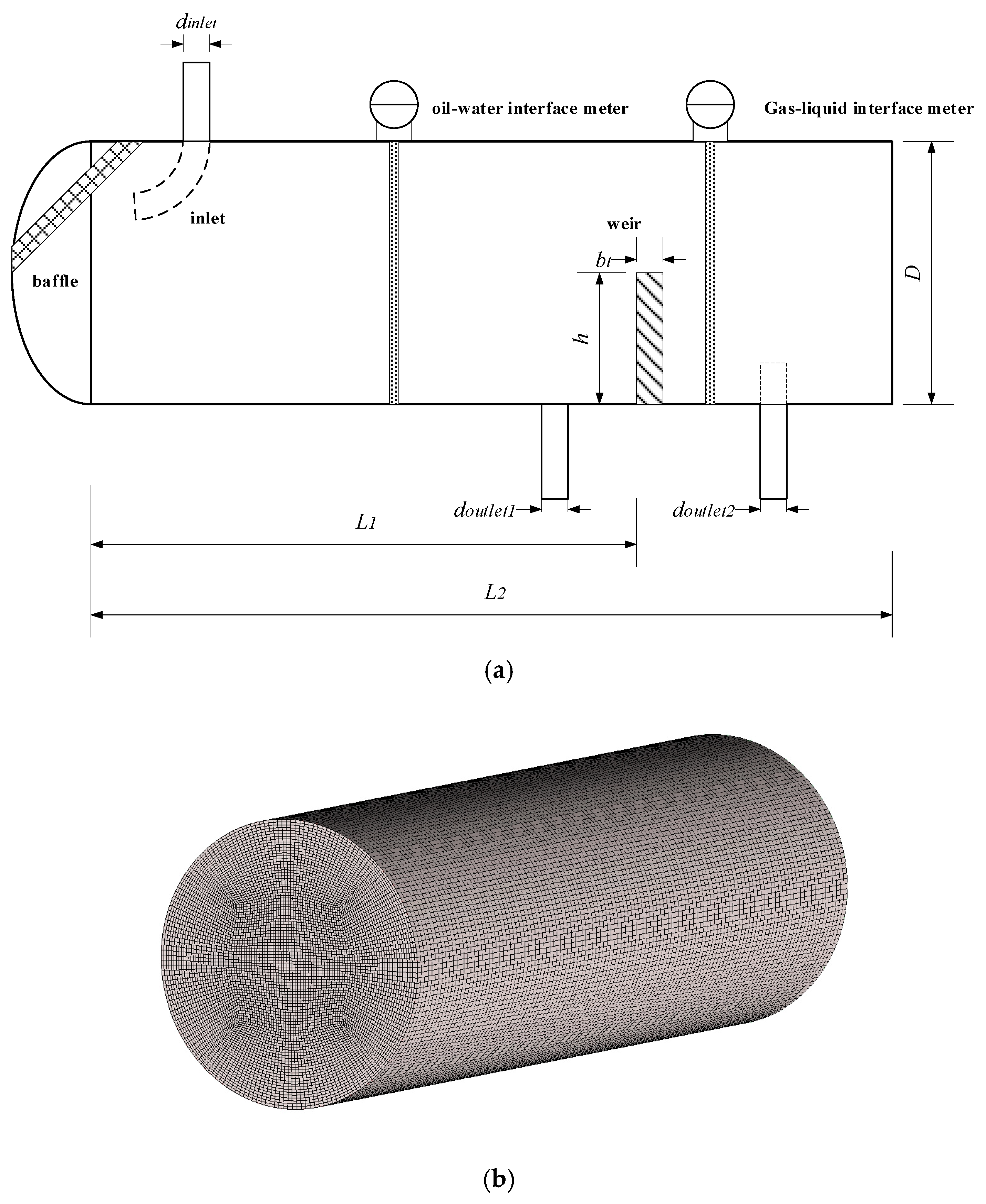
3.1. Separator

A schematic representation of the separator is shown in Figure 1a. The main body of the separator was fabricated using 304 stainless steel to withstand the maximum operating pressure of 10 MPa. The allowable stress for this material is specified as 137.8 MPa. To calculate the wall thickness δ_s required to ensure safe operation under design conditions, the following formula can be applied:

$${\delta }_s={\displaystyle \frac{P_S{D}_0}{2({[\sigma ]}^t{E}_i+PY)}},$$

(13)

where P_S is the design pressure, D₀ is the outer diameter of the separator vessel, [σ]^t is the allowable stress of the material, and E_i is the mass coefficient.

Assuming a conservative corrosion allowance of 1.5 mm, the calculated wall thickness ensures that the separator can operate reliably.

Based on the above calculations, the wall thickness δ_s greater than 27.5 mm was deemed necessary to meet the strength requirements; hence, the separator was manufactured with a wall thickness of 32.5 mm, providing a generous safety margin. The total length of the main body was approximately 1700 mm.

The weir thickness was specifically designed with consideration for the operating pressure of the separator with careful attention paid to weld strength. Consequently, a thickness of 26 mm was selected for the weir to ensure durability and reliability under the anticipated operational stresses.

The weir height was set to half the inner height of the separator, which is in accordance with the established design heuristics commonly found in most separator configurations. Inside the separator, the inner volume is divided into two distinct regions: an oil–water separation zone near the inlet and an oil-enriched zone located downstream of the weir. Accordingly, interface meters were strategically positioned in each area to accurately monitor phase stratification. An oil–water interface meter was installed in the oil–water separation zone to track the boundary between the water and oil phases, while a gas–liquid interface meter was deployed in the oil-enriched region to delineate the interface separating vapor from liquid fractions.

Following the principle of Reynolds number similarity, which is crucial for maintaining consistent flow patterns across different scales, the inlet and outlet pipes of the separator were designed with an inner diameter of 50 mm. The inlet of the separator was oriented toward the front end of the device, strategically incorporating a baffle to increase the likelihood of droplet collisions. This enhancement facilitated the coalescence of smaller droplets into larger aggregates, which were more conducive to gravitational settling.

3.2. Test Facility

The test facility consisted of five components: a circulating mixing system, an inflow pressurization system, a measurement system, a pressure environment control system, and a separator vessel. A P&ID of the test facility is shown in Figure 2.

The pressure environment control system includes decompression valves. Pressure sensors were strategically placed at a distance five times the pipe diameter upstream of the valves to continuously monitor the internal environmental pressure within the pipeline. Prior to experimentation, the set point values for the pressure sensors were programmed according to the test conditions. When the internal pressure of the pipeline did not reach this predefined value, the valve maintained a minimal leakage rate, allowing for a gradual increase in pressure before the valve. As the pressure rises and surpasses the set threshold, the valve aperture expands, regulating and stabilizing the front-end pressure at the designated level. This mechanism ensured precise control over the pressure environment throughout the experimental process, facilitating accurate testing under controlled conditions.

The experiments utilized compressed air, tap water, and formulated oil as working fluids. The formulated oil consisted of a predetermined mixture of diesel and crude oil. Prior to experimentation, stability tests were conducted on the formulated oils. Under simulated shear rates equivalent to those imposed during experiments, the formulated oil demonstrated rapid separation from water at atmospheric pressure, indicating satisfactory stability. The baseline conditions and parameters for each phase are listed in

Table 3. Phase parameters.

	Density (kg/m3)	Viscosity (mPa·s)	Content (%)
oil	827.3	7.2	9.1
water	998.5	1.001	90.9

. Four pressure gradients (0.5, 2, 4 and 6 MPa) were established for the experimental setup, while the temperature remained constant at 20 °C.

To ensure uniform shear states for every batch of mixed fluids, identical operating (2 min) and residence durations (6 min) were set. Adequate intervals were introduced to mitigate the cumulative effects of repeated shearing on the oil samples. Following the attainment of specified residence durations, samples were extracted after separation from the outlet tubing of the separator to evaluate and quantify separation efficacy.

3.3. Separation Effect Testing

The separation efficiency was evaluated based on the oil content in the effluent from the separator’s water outlet, encompassing the quantification of all adsorbed, dissolved, and adherent petroleum hydrocarbons present in the sampling container. The analytical procedure comprises the following steps.

• Step 1: The samples were placed in a hot water bath for oil solubilization with the heating temperature set at 70 °C for a preheating duration of 20 min.
• Step 2: The water samples were vigorously shaken to dislodge any wall-adherent materials, ensuring a homogeneous mixture of the specimens.
• Step 3: The prepared samples were transferred into a 50 mL stoppered spectrophotometer tube.
• Step 4: Upon reaching room temperature, the samples were acidified by adding 6N hydrochloric acid to achieve a pH of less than 2. Subsequently, 5 mL of n-hexane was introduced, the mixture was vigorously shaken, and then it was left undisturbed to facilitate phase separation.
• Step 5: The stratified liquids were extracted, and their absorbance was measured according to the oil standard curve. The oil content C was then determined by referencing the absorbance value against the same standard curve.

Figure 3 illustrates the process of sample settling and stratification.

The oil content of the water sample was calculated by Equation (14):

$$oiw=C{\displaystyle \frac{V_1}{V_2}},$$

(14)

where oiw is the oil content in the water sample, C is the oil content in the n-hexane extract, V₁ is the volume of the n-hexane extraction solvent, and V₂ is the volume of the original water sample.

3.4. Test Instruments

The measuring range of the interface meter spans from 0 to 645 mm, encompassing the full height of the separator, with a measurement error of 0.1%, boasting a resolution of 0.01 mm. Prior to the experiment, a mixture of oil and water was prepared to evaluate the accuracy and response time of the interface meter. Tests indicated that the interface meter could identify a mixture with over 10% oil content as the oil phase. For instantaneous interface changes, the response time of the interface meter does not exceed 3 s.

A turbine flow meter was utilized to monitor the flow rate with a maximum range of 15 m³/h and an error margin of ±0.15 m³/h. The pressure gauge used to monitor the internal environment of the separator has a range of 0 to 10 MPa with a measurement accuracy of 0.5%.

An infrared spectroscopic oil content analyzer was employed to assess the oil content in water samples with a measurement range of 0 to 1000 mg/L. To enhance the reliability of the test data, the samples are diluted to between 100 and 900 mg/L before the final determination of the oil content. The accuracy of the analyzer is ±2%.

3.5. Numerical Method and Simulation Settings

Computational Fluid Dynamics (CFD) is a powerful tool in the investigation and optimization of horizontal gravity-based multiphase separators, and it is widely utilized in design and enhancement studies related to these separators. Primarily employed to simulate the complex phase separation processes occurring within them, CFD allows designers to conceptualize and estimate the essential dimensions and structure of separators even without empirical initial data. The provision of clear visual representations illustrating the spatial distribution of distinct phases enables researchers to quickly identify opportunities for optimization, facilitating faster advancements in separator design.

In simulations, fluid property parameters are generally computed using two methods. One method treats the incoming fluid as a mixed phase, applying volume-averaged considerations for properties such as viscosity. The other employs the Volume of Fluid (VOF) method, tracking the behavior of sparse droplets of the dispersed phase through Lagrangian methods [24,30,31,32,33]. The tracking of the interface between the phases is accomplished by the solution of a continuity equation for the volume fraction of one of the phases. The equation is as follows:

$${\displaystyle \frac{1}{{\rho }_q}}\left[{\displaystyle \frac{\partial }{\partial t}}({\alpha }_q{\rho }_q)+\nabla \cdot ({\alpha }_q{\rho }_q{v}_q)\right]={\displaystyle \frac{1}{{\rho }_q}}({\dot{m}}_{pq}-{\dot{m}}_{qp}),$$

(15)

where ${\dot{m}}_{qp}$ is the mass transfer from phase q to phase p, and ${\dot{m}}_{pq}$ is the mass transfer from phase p to phase q. The subscript q refers to the qth phase; α_q is the volume fraction about the qth phase. The primary phase volume fraction will be computed based on the following equation:

$${\displaystyle \sum _{q=1}^n{\alpha }_q=1},$$

(16)

Numerical simulations were performed using FLUENT 2022. A geometric model was created based on the separator sample with the computational fluid domain represented as a cylinder measuring 545 mm in diameter and 1700 mm in length. To capture the variations in the stratification of the oil–water two-phase flow in the simulation results, a structured mesh was established for the model, consisting of approximately 860,000 elements as shown in Figure 1b. The distribution of the oil–water two-phase flow was extracted from the middle cross-section of the horizontal cylinder at the maximum vertical diameter, serving as the numerical calculation results, thus eliminating the influence of the wall. To more accurately simulate the phase separation process and better reproduce the phase interface, the Eulerian multiphase flow model was employed, which was combined with the VOF method to manage the phase boundary. Given that the oil-to-water ratio in the inlet stream is less than 1:10, the oil phase was designated as the dispersed phase. Factors influencing the oil–water interaction, including surface tension and drag forces, were considered.

The continuity equation and momentum conservation equation for multiphase flow models are formulated as follows:

$${\displaystyle \frac{\partial }{\partial t}}({\alpha }_q{\rho }_q)+\nabla \cdot ({\alpha }_q{\rho }_q{v}_q)=0,$$

(17)

$${\displaystyle \frac{\partial }{\partial t}}({\alpha }_q{\rho }_q{v}_q)+\nabla \cdot ({\alpha }_q{\rho }_q{v}_q{v}_q)=-{\alpha }_q\nabla P+\nabla \cdot {\tau }_q+{\alpha }_q{\rho }_{q}g+{\displaystyle \sum _{p=1}^n{R}_{pq}},$$

(18)

where R_pq is the interphase interaction force, which predominantly encompasses the drag force in this specific context.

The symmetric model was applied to solve for the interphase drag, which pertains to the interphase forces and interphase exchange coefficients, and can be expressed in the following form:

$$K_{pq}={\displaystyle \frac{{\alpha }_p({\alpha }_p{\rho }_p-{\alpha }_q{\rho }_q)f}{{\tau }_{pq}}},$$

(19)

where τ_pq represents the droplet relaxation time. The governing equation of relaxation time is as follows:

$${\tau }_{pq}={\displaystyle \frac{({\alpha }_p{\rho }_p-{\alpha }_q{\rho }_q){\left(\frac{d_p+d_q}{2}\right)}^2}{18({\alpha }_p{\mu }_p-{\alpha }_q{\mu }_q)}},$$

(20)

The drag function is

$$f={\displaystyle \frac{C_D\mathrm{Re}}{24}},$$

(21)

The equation for calculating the drag coefficient is

$$C_D=\{\begin{array}{cc}24(1+0.15{\mathit{Re}}^{0.687})/\mathrm{Re}& \hspace{1em}\mathrm{Re}\le 1000\hfill \\ 0.44& \hspace{1em}\mathrm{Re}>1000\hfill \end{array},$$

(22)

The flow field exists within a closed space; thus, wall boundary conditions were established. The settling velocity of droplets within the separator is low, so a laminar flow model was utilized for the simulations. The fluid domain is affected by gravity, causing the oil droplets to settle naturally.

We conducted unsteady calculations with a time step of 0.1 s and a simulation duration of 300 s to ensure the separation process was fully completed. The equations were discretized using higher-order schemes, and the calculation process was used to monitor changes in the phase content at various heights.

Regarding the setting of droplet sizes in the dispersed phase, due to the complexity of actual size distributions leading to excessive computational demands, a simplified approach was adopted. Specifically, this study employed an experimentally determined characteristic diameter as the representative average size for oil-phase simulation purposes. It is assumed that the droplet sizes remained constant throughout the computational domain, thus simplifying the rising process to one that varies linearly with respect to time and position. This approach has a minor influence when the emphasis of the study is on the variation in interface changes.

4. Results and Discussion

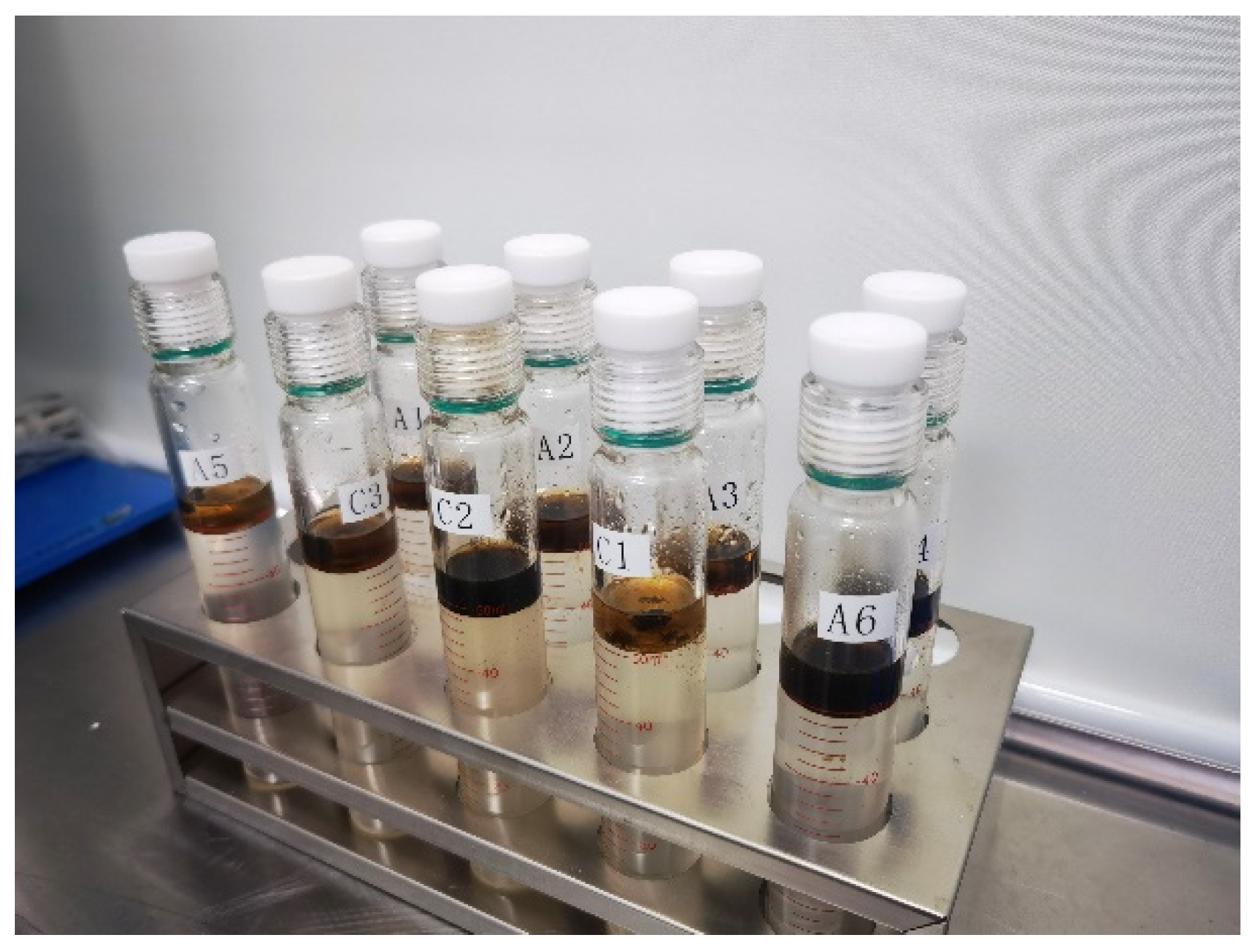
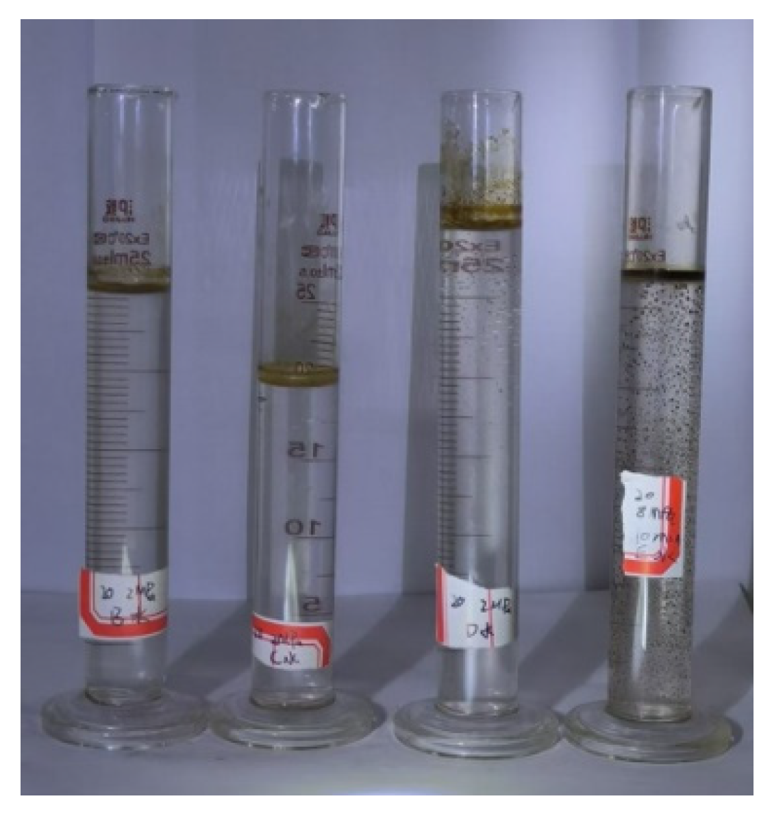
4.1. Test Results and Separation Effect

Test water samples were poured into graduated cylinders. After a brief period of quiescence, it was noted that the water samples appeared uniformly mixed, although those from the high-pressure experiments exhibited slightly lower clarity, as shown in Figure 4. After 24 h, only a few visible oil droplets or films had formed in the contents of the graduated cylinders. Following the protocol outlined in Section 3.3, analyses were performed on the separated test water samples, resulting in the findings presented in

Table 4. Oil content in the samples.

Pressure (MPa)	Oil Content (mg/L)
0.5	36.54
2	70.05
4	123.65
6	157.00

. Upon examination, the average oil content in the water sample was found to be 36.54 mg/L under atmospheric pressure separation testing. This value increased with higher experimental pressure, reaching an average oil content of 157.00 mg/L when the pressure was raised to 6 MPa. The concentration of oil in water is directly related to the degree of oil–water separation achievable within a given timeframe. Emulsions, defined by the uniform dispersion of tiny oil droplets surrounded by surfactant molecules, exhibit increased stability, making the separation of such mixtures more challenging. As droplet size decreases, the likelihood of oil droplets colliding and merging diminishes, resulting in a higher number of uniformly dispersed oil droplets within the water medium. When subjected to increased pressures, oil droplets in oil–water mixtures tend to decrease in size. This phenomenon promotes the formation of more finely divided emulsions, creating further challenges for effective oil droplet aggregation and coalescence.

Figure 5 shows the variations in oil content, from which it can be deduced that there is a linear relationship between oil content and pressure. Assuming identical operational parameters for the same separator, the efficiency of water treatment deteriorates linearly with an increase in pressure. Drawing from experimental data, it can be inferred that the separator’s ability to treat water can undergo preliminary evaluation through interpolative computations at arbitrary operating pressures. When pressure exceeds 10 MPa, predictions indicate that the oil concentration in water will surpass 250 mg/L. Such estimations reflect the overarching trend of oil droplet size transformation within the container, suggesting a compression effect on oil droplets under increased atmospheric pressure from an emulsion generation perspective.

The testing of oil content in water involves sampling, stirring, mixing, and conducting chemical analysis. Potential sources of error include the sample volume error, the n-hexane extraction volume error, and the instrument error of the oil content analyzer. Consequently, the relative variance of the test results is calculated as follows:

$${{\sigma }_{oiw}}^2=oi{w}^2({\displaystyle \frac{{\sigma }_{V_1}^2}{V_1^2}}+{\displaystyle \frac{{\sigma }_{V_2}^2}{V_2^2}})+{\sigma }_{in}^2,$$

(23)

where σ_oiw² represents the variance of the test data, σ_V1 denotes the sample volume error, σ_V2 signifies the n-hexane extraction volume error, and σ_in indicates the instrument error.

4.2. Analysis of Separation Performance

Given the horizontal cylindrical structure of the separator vessel, changes in the height of the oil–water interface trigger corresponding variations in the cross-sectional area. Thus, the height measurements directly obtained by the interface meter do not provide an immediate representation of the oil–water separation progress, necessitating adjustments to these raw interface heights. Taking the steady-state height of the oil–water interface during system operation as the baseline H₀, the overall volume V₀ of the water layer contained within the separator can be deduced accordingly. Let ΔH represent the fluctuation in the oil–water interface height throughout the experimentation, and let ΔV denote the resulting variance in the water layer volume. By standardizing the initial volume of the water layer, the ratio of the water layer volume change was utilized as a unified measure indicative of oil–water separation efficacy, which is reflected through modifications to the oil–water interface. Figure 6 illustrates the variations in the thickness of the water layer before and after detachment of the oil droplets. This methodology facilitates a systematic evaluation of oil–water interface dynamics. The ratio β is defined as

$$\beta ={\displaystyle \frac{f(\Delta H)}{f(H_0)}}={\displaystyle \frac{\Delta V}{V_0}},$$

(24)

Figure 7 illustrates the oil–water separation process across pressures ranging from 0.5 to 6 MPa. The separation procedure is divided into two stages. During stage 1, the ratio of the separated water volume shows a linear increase over time, reflecting the characteristic behavior of fixed-diameter oil droplets rising at consistent velocities. The slope of this line reflects the diameter of the dispersed oil droplets, indicating that larger droplets ascend more rapidly toward stability, which is a phenomenon consistent with the theory outlined in Equation (3). The duration of the volume growth stage corresponds to the time required for the lowest droplets to float upward and reach the oil–water interface.

Once the separation curve stabilizes, indicating the near-completion of the separation process, the system enters stage 2, which is characterized by a largely constant value. This stable value provides insight into the ultimate efficacy of oil–water separation, serving as a quantitative metric for evaluating the final outcome.

As pressure increases, the slope of stage 1 of the separation curve decreases. From the perspective of droplet size in the dispersed phase, this indicates that higher pressure results in a reduction in droplet diameter. This observation is intrinsically linked to the equilibrium established between the surface energy and kinetic energy concerning droplet size in the dispersed phase. Emulsions are generated spontaneously when the surface tension at oil–water interfaces becomes low [34,35,36,37]. In conventional multiphase flows, the formation of emulsions can primarily be attributed to the significant kinetic energy engendered by elevated shear rates, which can overcome the barrier posed by surface tension, instigating the fragmentation of the continuous phase into finer droplets. However, as the system approaches a state of equilibrium, the necessity to minimize free energy catalyzes the coalescence amongst these minuscule droplets, persisting until a stable stratification condition is achieved.

In Figure 7, the two stages of separation are distinguished by different colors. In Figure 7a, the duration of stage 1 lasts approximately 74 s. If the final volume of the separated water phase remains constant, then the higher the pressure, the longer the duration of stage 1. In Figure 7b,c, it is shown that despite increased pressures compared to Figure 7a, the duration of stage 1 decreases to roughly 58 and 66 s. This reduction is attributed to a significant shift in the stabilized oil–water interface position, resulting in shorter trajectories for oil droplets amid slowed settling rates. In Figure 7d, however, due to the exceptionally small dimensions of oil droplets, the length of stage 1 is significantly influenced by motion velocity, leading to an extended duration. Therefore, when evaluating the effectiveness of oil–water separation under pressured conditions, the stability of the emulsion layer becomes a crucial factor that warrants attention.

Some experimental investigations have been carried out to examine the changes in interfacial tension between selected hydrocarbons and other organic substances under high-pressure conditions and in contact with various media [38,39,40,41,42,43,44]. The results clearly indicate that as the pressure increases to several megapascals, the interfacial tension experiences a significant decrease, showing a direct correlation with rising pressure levels. Ultimately, this leads to the droplet size of the dispersed phase tending toward smaller dimensions under high-pressure conditions.

Figure 8 illustrates the separation process reconstructed via numerical simulation, where the y-axis depicts the vertical position within the upper half of the separator, and colors indicate varying water saturation levels. By extracting the isolines representing points with a water cut of 90% and comparing them against the scatter plot data indicative of the experimental measurements, it was found that the numerical simulation aligns well with the experimental outcomes. Specifically, the numerical results demonstrated a strong capability to emulate the detachment process of oil droplets from the water phase.

Figure 8a illustrates that the thickness of the emulsion layer during the separation process under low pressure varies by approximately 0.38 R. When the pressure increases to 2 MPa, as depicted in Figure 8b, the change in emulsion layer thickness is around 0.28 R. As the pressure continues to rise, the emulsion layer thickness further diminishes. It is evident that this layer thickness has a negative correlation with pressure. From the perspective of oil droplets, an increase in pressure decreases the average particle size of the droplets, resulting in a thicker and more stable emulsion layer, while the thickness of the oil–water mixed layer that can be separated within a specific timeframe becomes thinner. Considering the combined effects of the time response error and the measurement error of the interface meter, these two factors act independently, meaning the actual error in the interface data is a linear superposition of the two aforementioned errors. The impact of the total error is illustrated with error bars, and the graphs in Figure 8 indicate that the test values fall within the error range, demonstrating consistency with the numerical simulation of the high water content interface. The maximum error occurs at the initial moment of separation, not exceeding 8.5%.

Figure 9 presents a comparison between the interface measurement results and numerical simulations. It is apparent that all data points are close to the diagonal line with a relative error of less than 18%. This indicates that the numerical simulation results can effectively predict oil–water separation, although the prediction error at high pressure is slightly larger, remaining below 20% overall.

Based on numerical simulations, the following equation describing the mean droplet size of the dispersed oil phase as a function of pressure was proposed:

$$d_m=d_{m,0}\cdot e^{-0.14P},$$

(25)

where d_m is the mean droplet size at any given pressure; d_m,0 is the mean droplet size under atmospheric pressure; and P is the pressure.

4.3. Analysis of Droplet Evolution Process and Optimization of Separator Design

From the experimental test results, we can determine the time duration and layer height for stage 1 of the interface change between the oil and water phases, allowing us to calculate the velocity of the oil droplets. Equation (9) clarifies the relationship between oil droplet velocity and particle size, which is established through the analysis of drag force, thus emphasizing the crucial role of drag coefficient calculation in high-pressure separation scenarios to ensure the precision of oil droplet velocity determinations.

Sano [45] derived an expression for non-steady resistance on a spherical surface, considering the conditions for the pulsatile initiation of droplets. Mei and Adrian [46] also developed another formulation for total non-steady resistance under finite Reynolds numbers. The impact of internal recirculation within the droplets was also considered to improve the accuracy of the drag coefficient [47,48,49,50].

In this paper, based on the relationship between velocity and particle diameter, a correlation was developed to formulate the equation for calculating the drag coefficient:

$$C_D=16.8{(1+4.13\times {10}^3\sqrt{{\displaystyle \frac{{\mu }_c}{{\rho }_c{d}_m{V}_{sep}}}})}^2,$$

(26)

Under higher pressures, the reduced settling velocity of the droplets requires a longer residence time for the separator to operate effectively, prompting adjustments in the design dimensions, starting with updates to the droplet velocity figures. The diameter of the separator is revised concerning the ratio of settling times for equivalent settling distances, which is concurrently informed by studies on the relationship between emulsion thickness and dense packed layer or zone thickness [51], leading to corrections in the settling distance within the time-based calculations. Additionally, considerations must be given to the length-to-diameter ratios typical of pressure vessel designs when addressing the longitudinal dimensions of separators. Post revisions to both diameter and length, capacity constraints for each phase are established based on the incoming flow rate, guiding final adjustments to the overall dimensions of the separator.

Taking the experimental operating conditions and prototype parameters as an example, when the pressure rises to 8 MPa, the predicted droplet diameter decreases according to Equation (25) under the same inflow rate and operating temperature. Consequently, the droplet settling velocity, calculated iteratively using Equation (26), significantly decreases, resulting in a substantial increase in the residence time required by the separator. Subsequently, using Equation (12) as the primary basis for adjusting the separator dimensions, the diameter of the separator is increased by a factor of two, while the length becomes 2.15 times the original length, and the settling space is expanded to approximately 8.6 times that of the original separator. Therefore, it is crucial to rigorously calculate the parameters for deep-water separators, aiming to minimize their scale while ensuring effective separation.

5. Conclusions

An experimental investigation was conducted to examine the separation characteristics of a simulated deep-water horizontal separator. In the commonly used design process for three-phase separators in industry, particle size assumptions for the dispersed phase droplets in the continuous phases of gas and liquid are made based on experience, and Stokes’ law along with other movement regulations of dispersed phase particles in the continuous phase are utilized to analyze the flow velocity of the droplets, calculating the minimum residence time of each phase. The volume of each phase within the separator is designed to ensure that the droplets have adequate settling time, and the separator’s design size is determined by combined volumes of each phase. However, high-pressure conditions in deep water alter in the droplet settling process. Experimental observations indicate that an increase in pressure prolongs the droplet settling time, reflecting a decrease in the settling velocity of the dispersed phase droplets.

• Combined with the particle size analysis of oil droplets in water, as the pressure increased, the particle size of the dispersed phase oil droplets decreased, and the characteristic particle size of the droplet group decreased. Furthermore, according to the energy analysis, the surface tension of the oil droplets decreased under high pressure, further influencing the balance between the surface energy and kinetic energy of the droplets, leading to a reduction in the droplet size.
• The internal flow within the separator cannot be described as a simple laminar flow state. The high pressure intensifies the collisions of small droplets, raising questions about the applicability of Stokes’ law. The drag coefficient of the droplet sedimentation process was inferred from the oil–water separation characteristics, and the drag coefficient for high-pressure separation was adjusted using a correction formula. The droplet settling velocities at other pressures were simulated through calculations.
• The influence of high pressure on separator design is evident in the alterations to the dispersed phase settling process and emulsion layer. Under deep-water conditions, the reduction in droplet settling velocity necessitates an increase in the design size of the corresponding separator. Additionally, the changes in the emulsion layer require the conventional layer thickness criterion to have a larger safe operating margin under high pressure.

References

1. Wang, J.; Liang, J.; Zhao, Q.; Chen, J.; Zhang, J.; Yuan, Y.; Zhang, Y.; Dong, H. Characteristics of deepwater oil and gas distribution along the silk road and their controlling factors. Water 2024, 16, 240. [Google Scholar] [CrossRef]
2. Zhang, N.; Wang, Q.; Wang, J.; Hou, L.; Li, H. Characteristics of oil and gas discoveries in recent 20 years and future exploration in the world. China Pet. Explor. 2018, 23, 44–53. [Google Scholar]
3. Zhang, G.; Qu, H.; Zhang, F.; Chen, S. Major new discoveries of oil and gas in global deep-waters and enlightenment. Acta Pet. Sin. 2019, 40, 1–34, 55. [Google Scholar]
4. Wang, Z.; Wen, Z.; He, Z.; Chen, R.; Shi, H.; Chen, X. Characteristics and enlightenment of new progress in global oil and gas exploration in recent ten years. China Pet. Explor. 2022, 27, 27–37. [Google Scholar]
5. Gupta, R.K.; Dunderdale, G.J.; England, M.W.; Hozumi, A. Oil/water separation techniques: A review of recent progresses and future directions. J. Mater. Chem. A 2017, 5, 16025–16058. [Google Scholar] [CrossRef]
6. Van, S.L.; Van, D.T. Selection of an optimizing inlet angle for the gas-liquid cylindrical cyclone separator on hydrokinetic behavior. J. Adv. Mar. Eng. Technol. 2020, 44, 82–87. [Google Scholar]
7. Ghafoori, S.; Omar, M.; Koutahzadeh, N.; Zendehboudi, S.; Malhas, R.N.; Mohamed, M.; Al-Zubaidi, S.; Redha, K.; Baraki, F.; Mehrvar, M. New advancements, challenges, and future needs on treatment of oilfield produced water: A state-of-the-art review. Sep. Purif. Technol. 2022, 289, 120652. [Google Scholar] [CrossRef]
8. Jiang, W.; Hai, L.; Yang, X.; Liu, Y. Numerical study of swirl core-annular flow and factors influencing pressure drop in vertical pipelines for oi-water two-phase flow. Geoenergy Sci. Eng. 2025, 244, 213416. [Google Scholar] [CrossRef]
9. Kolla, S.S.; Mohan, R.S.; Shoham, O. Analysis of gas-liquid cylindrical cyclone separator with inlet modifications using fluid–structure interaction. J. Energy Resour. Technol.—Trans. ASME 2020, 142, 042003. [Google Scholar] [CrossRef]
10. Elhemmali, A.; Anwar, S.; Zhang, Y.; Shirokoff, J. A comparison of oil-water separation by gravity and electrolysis separation process. Sep. Sci. Technol. 2021, 56, 359–373. [Google Scholar] [CrossRef]
11. Zhang, T.; Li, C.; Sun, S. Effect of temperature on oil–water separations using membranes in horizontal separators. Membranes 2022, 12, 232. [Google Scholar] [CrossRef]
12. Fadaei, M.; Ameri, M.J.; Rafiei, Y.; Asghari, M.; Ghasemi, M. Experimental design and manufacturing of a smart control system for horizontal separator based on PID controller and integrated production model. J. Pet. Explor. Prod. Technol. 2024, 14, 2273–2295. [Google Scholar] [CrossRef]
13. Sulaiman, F.A.; Sidiq, H.; Kader, R. Liquid carry-over control using three-phase horizontal smart separators in Khor Mor gas-condensate processing plant. J. Pet. Explor. Prod. Technol. 2024, 14, 2413–2435. [Google Scholar] [CrossRef]
14. Stomquist, R.; Gustafson, S. SUBSIS-the world’s first subsea separation and injection system. World Pumps 1999, 3, 33–36. [Google Scholar] [CrossRef]
15. Denney, D. Perdido Development: Subsea and Flowline Systems. J. Pet. Technol. 2010, 62, 53–55. [Google Scholar] [CrossRef]
16. Arnold, K.; Stewart, M. Designing Oil and Gas Production Systems: How to size and select two-phase Separators. World Oil 1984, 199, 73. [Google Scholar]
17. Arnold, K.; Stewart, M. Designing oil and gas production systems: How to size and select three-phase separators. World Oil 1984, 199, 87. [Google Scholar]
18. Svrcek, W.Y.; Monnery, W.D. Design two-phase separators within the right limits. Chem. Eng. Prog. 1993, 89, 53–60. [Google Scholar]
19. Monnery, W.D.; Svrcek, W.Y. Successfully specify three-phase separators. Chem. Eng. Prog. 1994, 90, 29. [Google Scholar]
20. Gas Processors and Suppliers Association (GPSA). GPSA Engineering Data Book, 11th ed.; GPSA: Tulsa, OK, USA, 1998. [Google Scholar]
21. Watkins, R. Sizing separators and accumulators-speed with which operators can correct upsets is included in these design considerations. Hydrocarb. Process 1967, 46, 253–261. [Google Scholar]
22. Evert, O.G.; Matthew, J.R. Optimal design of two-and three-phase separators: A mathematical programming formulation. In Proceedings of the SPE Annual Technical Conference and Exhibition, Houston, TA, USA, 3–6 October 1999. [Google Scholar]
23. Ghaffarkhah, A.; Shahrabi, M.A.; Moraveji, M.K. 3D computational-fluid-dynamics modeling of horizontal three-phase separators: An approach for estimating the optimal dimensions. SPE Prod. Oper. 2018, 33, 879–895. [Google Scholar] [CrossRef]
24. Laleh, A.P.; Svrcek, W.Y.; Monnery, W.D. Design and CFD studies of multiphase separators—A review. Can. J. Chem. Eng. 2012, 90, 1547–1560. [Google Scholar] [CrossRef]
25. API. API SPEC 12J, Specification for Oil and Gas Separators, 8th ed.; API: Washington, DC, USA, 2008. [Google Scholar]
26. Davies, S.R.; Bakke, W.; Ramberg, R.M.; Jensen, R.O. Experience to date and future opportunities for subsea processing in statoilhydro. In Proceedings of the Offshore Technology Conference, Houston, TA, USA, 3–6 May 2010. [Google Scholar]
27. Capela Moraes, C.A.; da Silva, F.S.; Marins, L.P.M.; Monteiro, A.S.; de Oliveira, D.A.; Pereira, R.M.; Pereira, R.d.S.; Alves, A.; Raposo, G.M.; Orlowski, R.; et al. Marlim 3 phase subsea separation system: Subsea process design and technology qualification program. In Proceedings of the Offshore Technology Conference, Houston, TA, USA, 3–6 May 2012. [Google Scholar]
28. Orlowski, R.; Euphemio, M.L.L.; Euphemio, M.L.; Andrade, C.A.; Guedes, F.; Tosta da Silva, L.C.; Pestana, R.G.; de Cerqueira, G.; Loureno, L.; Pivari, A.; et al. Marlim 3 Phase Subsea Separation System—Challenges and Solutions for the Subsea Separation Station to Cope with Process Requirements. In Proceedings of the Offshore Technology Conference, Houston, TA, USA, 3–6 May 2012. [Google Scholar]
29. Shaiek, S.; Grandjean, L. Spoolsep for subsea produced water separation-experimental results. In Proceedings of the Offshore Technology Conference, Houston, TA, USA, 3–6 May 2015. [Google Scholar]
30. Tadros, T. Interparticle interactions in concentrated suspensions and their bulk (Rheological) properties. Adv. Colloid Interface Sci. 2011, 168, 263–277. [Google Scholar] [CrossRef]
31. Mason, T. New fundamental concepts in emulsion rheology. Curr. Opin. Colloid Interface Sci. 1999, 4, 231–238. [Google Scholar] [CrossRef]
32. Pal, R. Effect of droplet size on the rheology of emulsions. AIChE J. 1996, 42, 3181–3190. [Google Scholar] [CrossRef]
33. Mao, M.L.; Marsden, S.S. Stability of concentrated crude oil-in-water emulsions as a function of shear rate, temperature and oil concentration. J. Can. Pet. Technol. 1977, 16, PETSOC-77-02-06. [Google Scholar] [CrossRef]
34. Shchipunov, Y.A.; Schmiedel, P. Phase behavior of lecithin at the oil/water interface. Langmuir 1996, 12, 6443–6445. [Google Scholar] [CrossRef]
35. Pautot, S.; Frisken, B.J.; Cheng, J.; Xie, X.; Weitz, D.A. Spontaneous formation of lipid structures at oil/water/lipid interfaces. Langmuir 2003, 19, 10281–10287. [Google Scholar] [CrossRef]
36. González-Ochoa, H.; Ibarra-Bracamontes, L.; Arauz-Lara, J. Two-stage coalescence in double emulsions. Langmuir 2003, 19, 7837–7840. [Google Scholar] [CrossRef]
37. Sacanna, S.; Kegel, W.K.; Philipse, A.P. Spontaneous oil-in-water emulsification induced by charge-stabilized dispersions of various inorganic colloids. Langmuir 2007, 23, 10486. [Google Scholar] [CrossRef]
38. Fowkes, F.M. Determination of interfacial tensions, contact angles, and dispersion forces in surfaces by assuming additivity of intermolecular interactions in surfaces. J. Phys. Chem. 1962, 66, 382. [Google Scholar] [CrossRef]
39. Girifalco, L.A.; Good, R.J. A theory for the estimation of surface and interfacial energies. I. derivation and application to interfacial tension. J. Phys. Chem. 1957, 61, 904. [Google Scholar] [CrossRef]
40. Winterfeld, P.H.; Scriven, L.E.; Davis, H.T. An approximate theory of interfacial tensions of multicomponent systems: Applications to binary liquid-vapor tensions. AIChE J. 1978, 24, 1010–1014. [Google Scholar] [CrossRef]
41. Guggenheim, E.A. The principle of corresponding states. J. Chem. Phys. 1945, 13, 253–261. [Google Scholar] [CrossRef]
42. Queimada, A.J.; Rolo, L.I.; Caco, A.I.; Marrucho, I.M.; Stenby, E.H.; Coutinho, J.A.P. Prediction of viscosities and surface tensions of fuels using a new corresponding states model. Fuel 2006, 85, 874–877. [Google Scholar] [CrossRef]
43. Kiselev, S.B.; Ely, J.F. Generalized corresponding states model for bulk and interfacial properties in pure fluids and fluid mixtures. J. Chem. Phys. 2003, 119, 8645. [Google Scholar] [CrossRef]
44. Chhetri, A.B.; Watts, K.C. Surface tensions of petro-diesel, canola, jatropha and soapnut biodiesel fuels at elevated temperatures and pressures. Fuel 2013, 104, 704–710. [Google Scholar] [CrossRef]
45. Sano, T. Unsteady flow past a sphere at low Reynolds number. J. Fluid Mech. 1981, 112, 433–441. [Google Scholar] [CrossRef]
46. Mei, R.; Adrian, R.J. Flow past a sphere with an oscillation in the free-stream and unsteady drag at finite Reynolds number. J. Fluid Mech. 1992, 237, 323–341. [Google Scholar] [CrossRef]
47. Lin, Y.; Palmore, J. The effect of droplet deformation and internal circulation on drag coefficient. Phys. Rev. Fluids 2022, 7, 123602. [Google Scholar] [CrossRef]
48. Feng, J. A deformable liquid drop falling through a quiescent gas at terminal velocity. J. Fluid Mech. 2010, 658, 438–462. [Google Scholar] [CrossRef]
49. Harper, J.F.; Moore, D.W. The motion of a spherical liquid drop at high Reynolds number. J. Fluid Mech. 1968, 32, 367–391. [Google Scholar] [CrossRef]
50. Helenbrook, B.T.; Edwards, C.F. Quasi-steady deformation and drag of uncontaminated liquid drops. Int. J. Multiph. Flow 2002, 28, 1631–1657. [Google Scholar] [CrossRef]
51. Oshinowo, L.M.; Vilagines, R.G. Modeling of oil–water separation efficiency in three-phase separators: Effect of emulsion rheology and droplet size distribution. Chem. Eng. Res. Des. 2020, 159, 278–290. [Google Scholar] [CrossRef]
Figure 1. Description of separator: (a) the schematic of the separator; (b) mesh of the separator.
Processes 12 02619 g001
Figure 2. Experimental system.
Processes 12 02619 g002
Figure 3. The samples at rest following the extraction process.
Processes 12 02619 g003
Figure 4. Test water samples. (Sampled from water out with pressure labeled).
Processes 12 02619 g004
Figure 5. Oil content in the samples.
Processes 12 02619 g005
Figure 6. Schematic illustration of changes in the water layer.
Processes 12 02619 g006
Figure 7. Variation in the volume of separated water: (a) P = 0.5 MPa; (b) P = 2.0 MPa; (c) P = 4.0 MPa; (d) P = 6.0 MPa.
Processes 12 02619 g007
Figure 8. Simulation of oil–water separation process: (a) P = 0.5 MPa; (b) P = 2.0 MPa; (c) P = 4.0 MPa; (d) P = 6.0 MPa.
Processes 12 02619 g008
Figure 9. Simulated water layer versus measured water layer.
Processes 12 02619 g009