Dynamic Integrated Scheduling of Production Equipment and Automated Guided Vehicles in a Flexible Job Shop Based on Deep Reinforcement Learning

Abstract

The high-quality development of the manufacturing industry necessitates accelerating its transformation towards high-end, intelligent, and green development. Considering logistics resource constraints, the impact of dynamic disturbance events on production, and the need for energy-efficient production, the integrated scheduling of production equipment and automated guided vehicles (AGVs) in a flexible job shop environment is investigated in this study. Firstly, a static model for the integrated scheduling of production equipment and AGVs (ISPEA) is developed based on mixed-integer programming, which aims to optimize the maximum completion time and total production energy consumption (EC). In recent years, reinforcement learning, including deep reinforcement learning (DRL), has demonstrated significant advantages in handling workshop scheduling issues with sequential decision-making characteristics, which can fully utilize the vast quantity of historical data accumulated in the workshop and adjust production plans in a timely manner based on changes in production conditions and demand. Accordingly, a DRL-based approach is introduced to address the common production disturbances in emergency order insertions. Combined with the characteristics of the ISPEA problem and an event-driven strategy for handling dynamic events, four types of agents, namely workpiece selection, machine selection, AGV selection, and target selection agents, are set up, which refine workshop production status characteristics as observation inputs and generate rules for selecting workpieces, machines, AGVs, and targets. These agents are trained offline using the QMIX multi-agent reinforcement learning framework, and the trained agents are utilized to solve the dynamic ISPEA problem. Finally, the effectiveness of the proposed model and method is validated through a comparison of the solution performance with other typical optimization algorithms for various cases.

1. Introduction

With the implementation of various intelligent manufacturing strategies around the world, such as Industry 4.0, Made in China 2025, and New Robot Strategy, the manufacturing workshop is rapidly transitioning towards intelligent operation and maintenance. The flexible job shop is a highly adaptable and efficient organizational method for production systems, commonly employed in sophisticated manufacturing sectors such as the semiconductor, biopharmaceutical, and aerospace industries. A previous study has demonstrated that production scheduling is an effective measure for achieving energy-efficient production on the shop floor at the manufacturing system level [1,2,3,4,5]. Nevertheless, most work on production scheduling problems concentrated on static scheduling, which usually assumes that the information related to humans, workpieces, and equipment is predetermined and known. In actual production, there are frequently an immense amount of dynamic uncertainties, such as machine failures, emergency order insertion, and process completion time fluctuations, making it difficult to strictly execute scheduling plans formulated by static scheduling [6]. In contrast, dynamic scheduling not only addresses unforeseen situations in the manufacturing process, but it also entails the ability to respond quickly and adjust production plans to minimize the impact of these uncertain factors on production efficiency and cost. Therefore, it is of more practical significance to study dynamic scheduling.

In addition, a workshop manufacturing system consists of plenty of energy-consuming manufacturing resources. Automated guided vehicles (AGVs) have been widely applied for material handling in flexible job shops due to their benefits of flexibility, high precision, and high dependability [7]. In the current research on flexible job shop scheduling problems (FJSPs), it is commonly assumed that there are unlimited material transport resources. However, on the real shop floor, the unavailability of material handling resources and the early or delayed completion of material handling tasks can disrupt the operation plan of processing equipment [8], thereby affecting the feasibility of scheduling plans. Moreover, the current research on energy-efficient production scheduling usually focuses solely on the energy consumption (EC) of processing equipment and neglects the EC of material handling equipment like AGVs, robots, and conveyors. Hence, if the impact of material handling can be considered in production scheduling, i.e., through the integrated scheduling of production equipment and AGVs (ISPEA), this will be beneficial to enhancing the efficiency of processing and material handling resources simultaneously, as well as enhancing the potential of energy-efficient production in a workshop. With the rapid development of information technology, the application of the Internet of Things (IoT), manufacturing execution systems (MESs), and advanced planning and scheduling (APS) systems provides real-time data support for on-site workshop management and promotes the flow and sharing of information, which makes ISPEA feasible. Thus, considering the influence of the material handling processes executed by AGVs, this study aims to investigate the ISPEA problem, and design an effective solution method to obtain the optimal integrated scheduling scheme.

Currently, existing ISPEA studies usually ignore the disturbances to the formulation of scheduling plans caused by dynamic events and lack consideration of EC or EC-related optimization objectives. Furthermore, the ISPEA problem in a flexible job shop involves not only machine allocation and the sorting of job processing, but also involves transport processes that link different job operations. Therefore, it is more complex than the traditional production equipment-based FJSP and poses a challenge to the “model + algorithm” idea commonly utilized in the current research on workshop production scheduling. Meanwhile, the rapid advancement of the Internet of Things, big data, artificial intelligence (AI), and other emerging digital technologies has facilitated the collection and analysis of diverse data and information in manufacturing workshops. Reinforcement learning, including deep reinforcement learning (DRL), is adept at utilizing the extensive historical data collected and accumulated in the workshop to address sequential decision-making problems, which provides new ideas for addressing issues related to workshop production scheduling. As an algorithm capable of self-learning and optimizing decisions, RL can dynamically adjust production plans based on real-time production conditions and demand changes, and some further exploration has validated its advantages in solving dynamic scheduling problems [9].

Despite the many types of dynamic events, emergency order insertions are the focus of this study, and an event-driven strategy that allows for real-time monitoring and processing is proposed to handle them effectively. Therefore, the ISPEA problem studied in this paper can also be interpreted as an extension of the FJSP that comprehensively considers the impact of logistics and dynamic events, as well as the energy-efficient production needs. Accordingly, the DRL can be introduced to solve this better.

The rest of the paper is organized in the following manner: Section 2 provides an overview of the existing research related to ISPEA in flexible job shops. Section 3 presents the ISPEA problem model. Section 4 describes the process and specific steps of the multi-agent reinforcement learning (MARL) method, QMIX, employed to solve the ISPEA problem. The experimental findings are shown in Section 5. Section 6 summarizes the study and outlines future research directions.

2. Literature Review

In this section, current work related to dynamic ISPEA in a flexible job shop is reviewed from three aspects, i.e., energy-efficient scheduling, dynamic scheduling, and integrated scheduling, considering the impact of logistics factors, and the research gap motivated this study is analyzed.

2.1. Energy-Efficient Scheduling

In recent years, the energy-efficient scheduling problem for flexible job shops has increasingly become a research hotspot in the manufacturing field [10,11]. From the perspective of solution methods, there are four main types: heuristic algorithms, meta-heuristic algorithms, hyper-heuristic algorithms, and artificial intelligence methods.

Heuristic algorithms refer to strategies constructed based on intuition or experience to generate acceptable and feasible solutions for specific problems, generally called scheduling rules. It is widely accepted that no single scheduling rule can handle all scenarios and objectives, and composite scheduling rules usually perform better than simple rules across most objectives. Meta-heuristic algorithms are computational-intelligence-based methods for solving complex optimization problems, including evolutionary computation and swarm intelligence. Luo et al. [12] proposed a multi-objective grey wolf optimization (MOGWO) algorithm to solve an FJSP with EC and makespan as optimization objectives, and an experimental study based on 35 benchmark cases showed that the proposed MOGWO algorithm outperforms the representative multi-objective evolutionary algorithms such as the non-dominated sorting genetic algorithm-II (NSGA-II) and strength Pareto evolutionary algorithm-II (SPEA-II). Zhang et al. [13] employed a machine turning-off/on energy-saving strategy, and proposed an NSGA-II-based method for an FJSP with production EC and makespan as the optimization objectives. The experimental research not only verified the effectiveness of the energy-saving strategy, but also the effectiveness of the proposed solution method, through comparison with the ant colony optimization (ACO) algorithm, modified genetic algorithm (MGA), and genetic algorithm-particle swarm optimization (GA-PSO) algorithm. Wu et al. [14] developed a multi-objective FJSP model with generalized EC and makespan as the optimization objectives, and proposed a multi-objective simulated annealing algorithm to solve it. The numerical experiments verified that the proposed algorithm can effectively and efficiently solve the established model. Liu et al. [15] introduced a modified biology migration algorithm (MBMA) to minimize workshop EC; this algorithm can directly search the discrete scheduling space and balance its exploration capabilities by incorporating discrete migration operators based on crossover operations and a dynamic adjustment strategy for transition probabilities. Hyper-heuristic algorithms can automatically design scheduling rules using strategies such as genetic programming and gene expression programming, which have been utilized for solving energy-efficient FJSPs. Zhang et al. [16] employed gene expression programming to mine effective energy-saving rules, and proposed a mixed-integer linear programming model, incorporating the shutdown/restart energy-saving strategy, to minimize total energy consumption. Correspondingly, the search space for problem solutions was expanded, and the quality of the solutions was improved through multi-gene representation and self-learning mechanisms. Artificial intelligence methods, such as machine learning, game theory, multi-agent systems, and digital twins, have been gradually applied in production scheduling. Rakovitis et al. [17] established a new energy-efficient FJSP model and proposed a group-based decomposition method for solving large-scale problems. Furthermore, experiments demonstrated that the proposed approach can find feasible solutions with a lower EC for large-scale instances in a shorter computation time (within 10 min), and the EC can be reduced by up to 43.1% compared with the existing gene-expression programming-based algorithm. Zhang et al. [18] proposed a bi-level scheduling method based on dynamic game theory to address an FJSP for optimizing makespan, total EC, and machine load simultaneously, and the experiment revealed that when compared with the GA+ periodic scheduling method, the proposed method can minimize such three optimization objectives by 4.5%, 9.3%, and 8.75%, respectively. Zhou et al. [19] introduced an AI scheduler that improves learning efficiency by designing composite reward functions and solves the multi-objective performance enhancement issue in production scheduling, and the experimental results reveal the proposed strategy delivers excellent performances in terms of both decision accuracy and schedule repair.

Overall, the aforementioned studies have indicated that production scheduling is an effective measure for achieving energy-efficient production in flexible job shops from a manufacturing system perspective. Meta-heuristic algorithms are currently the mainstream methods for solving energy-efficient FJSPs, but they often fail to effectively utilize the rich production data generated during the operation of intelligent workshops and rarely consider the impact of dynamic events.

2.2. Dynamic Scheduling

Dynamic scheduling work can be categorized according to the types of dynamic disturbances in the workshop production process: job-related dynamic events, machine-related dynamic events, and other dynamic events [20]. Job-related dynamic events include random job arrivals, uncertain processing times, and urgent job insertions. Machine-related dynamic events usually encompass machine failures and machine overloads. RL and DRL have significant advantages in handling complex decision-making and optimization problems, providing new approaches and methods for addressing dynamic scheduling problems. Based on the types of dynamic events that are addressed, the research on adopting RL and DRL to handle dynamic scheduling problems in flexible job shops is summarized as follows.

Regarding the handling of job-related dynamic events, Bouazza et al. [21] utilized a Q-learning algorithm combined with scheduling rules to solve dynamic FJSPs with new job insertions. Liu et al. [22] proposed a double deep Q-network (DDQN) algorithm with a hierarchical and distributed architecture to address dynamic scheduling problems considering job arrival times in flexible job shops, and an alternative reward-shaping technique was introduced to improve learning efficiency and scheduling results. The simulation results showed that the proposed method outperformed existing scheduling strategies and maintained its advantages even when the manufacturing system configuration changed. Zhou et al. [23] presented a DRL-based method to minimize the makespan when new tasks arrive in a dynamic flexible job shop, and a deep Q-network (DQN) agent was used to select appropriate services from all candidate services for each arriving task. Further, two case studies with different task interval probabilities were utilized to illustrate the usefulness and efficiency of the proposed method.

Regarding the handling of machine-related dynamic events, Zhao et al. [24] proposed an improved Q-learning algorithm to address machine failure issues. Based on the initial scheduling plan generated by the genetic algorithm, the proposed algorithm integrated dynamic event information related to machine failures and selected the operations that were to be executed and the alternative processing equipment through a Q-learning agent. The experimental results showed that this approach significantly reduced job delay times in high-frequency dynamic environments compared with a single scheduling rule. Zhang et al. [25] utilized the proximal policy optimization (PPO) algorithm to deal with job shop scheduling problems under sudden machine failure conditions, and different types of reward functions were designed to guide scheduling agents in learning strategies that met the multi-objective optimization requirements, e.g., production efficiency and order waiting time. Compared with other scheduling rules and DRL algorithms, the PPO algorithm demonstrated superiority in convergence performance and achieving various scheduling optimization goals, and can obtain more desirable scheduling outcomes.

Focusing on the ability to handle multiple types of dynamic events simultaneously, Shahrabi et al. [26] combined the Q-factor algorithm with RL to tackle dynamic job shop scheduling problems involving random job arrivals and machine failures. Compared with the generalized variable neighborhood search algorithm and traditional scheduling rule-based methods, this solution achieved significant performance improvements and demonstrated stronger adaptability and optimization capabilities. Li et al. [27] aimed to minimize the makespan by systematically considering four typical dynamic events: new order arrivals, machine failures, order cancellations, and changes in order processing times. A rescheduling method based on Monte Carlo tree search (MCTS) was designed accordingly and compared with completely reactive scheduling methods and the GA-based rescheduling method through experiments. The experimental results indicated that the proposed method was an efficient and promising dynamic scheduling method, both in terms of solution quality and computational efficiency. Zhang et al. [28] designed a multi-agent PPO algorithm. Within this algorithm framework, multiple agents collaborated and competed to cope with the impact of random job arrivals and machine failures on job shop scheduling, thereby improving the efficiency and quality of the scheduling decisions. The experimental results show that the proposed method outperforms genetic programming (GP), DQN, and dispatching rules in terms of production strategy learning and disturbance handling.

The above research efforts have demonstrated the feasibility of RL and DRL in handling dynamic scheduling problems for flexible job shops. Compared with traditional research based on meta-heuristic and hyper-heuristic algorithms, these methods have certain advantages, increasing the response speed to dynamic events, reducing interruptions caused by dynamic events, and handling multiple types of dynamic events simultaneously. The inherent dynamic adaptability of RL/DRL methods presents a promising outlook for solving dynamic scheduling problems.

2.3. Integrated Scheduling

Material handling is crucial for the smooth transition of the workshop production process, but previous research on workshop production scheduling mainly focused on processing equipment, and the impact of logistics factors was mostly ignored or simplified. Therefore, the solutions to integrated scheduling problems are similar to those of processing equipment-oriented FJSPs. Gnanavel et al. [29] investigated the integrated scheduling of machines and AGVs in a flexible manufacturing system, developed a meta-heuristic differential evolutionary (DE) algorithm to address it, and conducted extensive testing to verify the effectiveness of the algorithm. Zhong et al. [30] decomposed AGV-machine joint scheduling into two strongly related sub-decisions (job sequencing and AGV selection) and constructed a combined rule generation framework. Accordingly, various combined rules could be generated by embedding diverse heuristic rules into the framework. Furthermore, the effectiveness of the involved Gurobi solver and combinatorial rule generation algorithm framework was verified using instances with different production characteristics, such as layout schemes and task scales. Gurobi generally performed better than the combination rule algorithm when seeking exact solutions for small-scale instances, but the performance gap narrowed at low AGV speeds. Meanwhile, the combinatorial rule generation algorithm outperformed Gurobi in terms of computation time when searching for exact solutions for large-scale instances. Li et al. [31] developed a hybrid deep Q-network (HDQN) to address dynamic multi-objective FJSPs in the case of insufficient transport resources, and the experimental results showed that the HDQN was superior and had greater generality compared with the incomplete HDQN, Q-learning using self-organizing maps, and HDQN using common rules, and can effectively deal with disturbance events and unseen situations through learning. Yuan et al. [32] introduced an enhanced DDQN approach to address FJSPs with AGVs to minimize the maximum completion time, and the calculation experiment results based on the self-built case demonstrated the accuracy and effectiveness of the proposed algorithm. Additionally, Sun et al. [33] proposed a RL scheduling method based on two-dimensional proximal policy optimization algorithms (2D-PPO) for the joint scheduling problem of AGVs and machines in job shops. Furthermore, three separate experiments revealed that the proposed 2D-PPO algorithm exhibited a better convergence performance and learning effect than the PPO with one-dimensional actions, achieved better solutions than the multi-agent system (MAS) algorithm for small-scale problems, and outperformed the single scheduling rule-based method for large-scale problems.

Note that most of the current research on ISPEA belongs to the category of static scheduling and lacks consideration of EC and EC-related environmental factors. These related efforts have demonstrated the feasibility and advantages of RL/DRL methods in solving dynamic ISPEA problems. However, RL/DRL methods also have certain limitations and potential biases. Their efficiency is determined by elements such as environment modeling accuracy, reward function design, and hyper-parameter selection, and inappropriate settings may result in unstable learning processes and a decrease in generalization ability. When used to handle dynamic events, they often require extensive basic training data and time to adapt to new situations, posing challenges for their use in manufacturing settings with low levels of informatization and intelligence. Furthermore, the current utilization of RL/DRL methods to address FJSPs and ISPEA is often based on a single agent, which leads to substantial issues in problem-solving efficiency, interaction with the environment, and adaptability as the complexity of the scheduling problems increases. In terms of problem characteristics, the present use of RL/DRL for production scheduling mainly focuses on single-objective optimization problems (SOPs). When multiple scheduling objectives need to be optimized simultaneously, the weighted sum method is commonly employed to transform a multi-objective optimization problem (MOP) into an SOP, which subsequently guides the design of the reward functions. Nevertheless, the weight coefficients of these optimization objectives are usually assigned fixed values, limiting the search range for the optimal solutions of an MOP. Therefore, when utilizing RL/DRL to deal with ISPEA problems, it is necessary to comprehensively consider its advantages and limitations to guarantee its effectiveness and practicality.

To summarize, in addition to processing equipment, transport equipment is also a significant energy-consuming resource in a workshop. Compared with traditional processing equipment-oriented production scheduling, the ISPEA is beneficial to the further expansion of the energy-saving potential of a manufacturing system. To meet the needs of practical production and enhance the sustainability of the manufacturing industry, ISPEA research should not only consider the impact of dynamic events but also pay attention to energy-efficient production. With the rapid development of AI technology, MARL has significant advantages in the completion of complex tasks through collaboration, adversarial learning, and improving generalization ability. As ISPEA problems are more sophisticated than traditional FJSPs, it is worth exploring the application of MARL to deal with ISPEA problems.

3. Problem Description and Modeling

The ISPEA problem in a flexible job shop involves n jobs that can be processed on m machines, and the transfer of job-related workpieces between different machines is executed by q AGVs with the same transport capacity. Job i (i = 1, 2, …, n) consists of l_i machining operations and each operation O_ij (j = 1, 2, …, l_i) can be processed on several alternative machine tools, whose quantity is denoted as N_ij. The processing time and EC for the same operation differ with the machine selected. Additionally, the standby power of different machines can vary. After a certain operation of a job (not the last operation) is completed, if the machine selected to execute its next operation is different from the one used to complete the current operation, an AGV will be needed to transport the workpiece associated with this job between the various machines. Correspondingly, the EC concerned in this study is not only related to the machines but also to the AGVs. Therefore, the ISPEA is to optimize the makespan and total EC simultaneously by selecting suitable machines and AGVs for jobs and rationally arranging the processing sequence of the operations allocated to each machine and the transport sequence of the job-related workpieces allocated to each AGV. Based on the research hypotheses for classical FJSP [34], the assumptions made for the ISPEA are as follows:

(1)

All jobs, machines, and AGVs are available at time zero. All jobs have the same priority, and the same goes for the AGVs.

(2)

The operations of each job must be processed sequentially according to the predetermined process specifications, and there is no processing sequence constraint between the operations of different jobs.

(3)

Machines are independent, and each machine can process only one job at a time. Once a job begins to be executed on a machine, it cannot be interrupted or canceled, and machine failure is not considered.

(4)

Each operation only needs one machine.

(5)

The machine is in standby mode while waiting for jobs and is not allowed to be powered off.

(6)

The capacity of each machine buffer for loading and unloading workpieces is infinite.

(7)

Each AGV has sufficient power. During transport, AGVs cannot be interrupted, and the impact of path conflicts and speed changes are not considered. After a transport task is completed, the corresponding AGV’s transport capacity is released.

(8)

If a workpiece requires transport, the loading and unloading time is included in the AGV transport time. Similarly, the auxiliary time of an operation performed on a machine (e.g., clamping and inspection time) is included in its processing time.

(9)

All AGVs are single-load ones, and each job-related workpiece can only be assigned to a single AGV if transport is needed.

Based on the research hypothesis, the symbols and definitions required for describing the static ISPEA problem, i.e., regardless of the disturbance of dynamic events in production, are shown in

Table 1. List of indices, sets, parameters, and variables.

Type	Symbol	Definition
Index & Set	h	Index of AGV; h = 1, 2, …, q
	i, i’	Index of job; i, i’ = 1, 2, …, n
	j, j’	Index of operation; j = 1, 2, …, li; j’ = 1, 2, …, li’
	k, k*	Index of machine; k, k* = 1, 2, …, m
	Nk	Set of operations that can be processed on machine k
Parameter	li	Number of operations of job i
	m	Number of machines
	n	Number of jobs
	Nij	Number of machines that can process Oij
	$P_h^{\mathrm{A}}$	Average transport power of AGV h
	$P_h^{\mathrm{I}}$	Standby power of AGV h
	$P_k^{\mathrm{I}}$	Standby power of machine k
	$P_k^{\mathrm{M}}$	Average processing power of machine k
	q	Number of AGVs
	$T_{ijk}^{\mathrm{M}}$	Processing time of Oij on machine k
	$T_{k{k}^{*}}^{\mathrm{A}}$	$\mathrm{Transport} \mathrm{time} \mathrm{of} \mathrm{an} \mathrm{AGV} \mathrm{travelling} \mathrm{from} \mathrm{machine} k \mathrm{to} \mathrm{machine} k^{*}; \mathrm{when} k=k^{*}, T_{k{k}^{*}}^{\mathrm{A}}=0$
	$C_{ij}^{\mathrm{A}}$	Completion time of transporting the workpiece related to job i to the machine executing Oij
Variable	$C_{\max }^{\mathrm{A}}$	Maximum transport completion time
	$C_{ij}^{\mathrm{M}}$	Processing completion time of Oij
	Cmax	Maximum completion time for all jobs
	EI	Total standby EC of all machines
	EM	Total processing EC of all machines
	ES	Total standby EC of all AGVs
	ET	Total transport EC of all AGVs
	$S_{ij}^{\mathrm{A}}$	Start time of transporting the workpiece related to job i to the machine executing Oij
	$S_{ij}^{\mathrm{M}}$	Processing start time of Oij
	$T_h^{\mathrm{I}}$	Total standby time of AGV h
	$T_k^{\mathrm{I}}$	Total standby time of machine k
	Xijk	1 if Oij selects machine k for processing and 0 otherwise
	$Y_{iji’j’k}$	$1 \mathrm{if} O_{ij} \mathrm{and} O_{i’j’}$$\mathrm{are} \mathrm{processed} \mathrm{on} \mathrm{machine} k \mathrm{and} O_{ij} \mathrm{is} \mathrm{executed} \mathrm{before} O_{i’j’}$, and 0 otherwise
	Zijh	1 if the execution of Oij requires transporting the corresponding workpiece and AGV h is selected, and 0 otherwise

.

The makespan of all jobs can be expressed as follows:

$$C_{\max }=\underset{i,j}{\max }\{C_{ij}^{\mathrm{M}}\}$$

(1)

The maximum transport completion time can be acquired as follows:

$$C_{\max }^{\mathrm{A}}=\underset{i,j}{\max }\{C_{ij}^{\mathrm{A}}\}$$

(2)

Accordingly, the total production EC for completing all jobs (E_total, J) is composed of the EC of machines and AGVs, which can be further expressed as follows:

$$E_{\mathrm{total}}=E_{\mathrm{I}}+E_{\mathrm{M}}+E_{\mathrm{S}}+E_{\mathrm{T}}$$

(3)

Owing to the constant machine standby power, it is necessary to obtain $T_k^{\mathrm{I}}$ to evaluate E_I. $T_k^{\mathrm{I}}$ can be calculated by

$$T_k^{\mathrm{I}}=\max \{C_{ij}^{\mathrm{M}}\}-\min \{S_{ij}^{\mathrm{M}}\}-{\displaystyle {\sum }_{i=1}^n{\displaystyle {\sum }_{j=1}^{l_i}{T}_{ijk}^{\mathrm{M}}}}$$

(4)

Similarly, evaluating E_S requires obtaining $T_h^{\mathrm{I}}$ first, which can be expressed as follows:

$$T_h^{\mathrm{I}}=\max \{C_{ij}^{\mathrm{A}}\}-\min \{S_{ij}^{\mathrm{A}}\}-{\displaystyle {\sum }_{i=1}^n{\displaystyle {\sum }_{j=1}^{l_i}(C_{ij}^{\mathrm{A}}-S_{ij}^{\mathrm{A}})}}, \forall h,i,j:Z_{ijh}=1$$

(5)

Then, the EC components of E_total can be specifically represented as follows:

$$E_{\mathrm{I}}={\displaystyle {\sum }_{k=1}^m\left(P_k^{\mathrm{I}}{T}_k^{\mathrm{I}}\right)}$$

(6)

$$E_{\mathrm{M}}={\displaystyle {\sum }_{i=1}^n{\displaystyle {\sum }_{j=1}^{l_i}{\displaystyle {\sum }_{k=1}^m\left(X_{ijk}{P}_k^{\mathrm{M}}{T}_{ijk}^{\mathrm{M}}\right)}}}$$

(7)

$$E_{\mathrm{S}}={\displaystyle {\sum }_{h=1}^q\left(P_h^{\mathrm{I}}{T}_h^{\mathrm{I}}\right)}$$

(8)

$$E_{\mathrm{T}}={\displaystyle {\sum }_{h=1}^q{\displaystyle {\sum }_{i=1}^n{\displaystyle {\sum }_{j=1}^{l_i}\left[Z_{ijh}{P}_h^{\mathrm{A}}(C_{ij}^{\mathrm{A}}-S_{ij}^{\mathrm{A}})\right]}}}$$

(9)

Therefore, the optimization objectives of the static ISPEA problem are presented as

$$\{\begin{array}{l}\mathrm{Minimize}[E_{\mathrm{total}}]\\ \mathrm{Minimize}[C_{\max }]\end{array}$$

(10)

subject to

$$C_{ij}^{\mathrm{M}}-S_{ij}^{\mathrm{M}}\ge {\displaystyle \sum _{\{k:O_{ij}\in N_k\}}\left(T_{ijk}^{\mathrm{M}}{X}_{ijk}\right)},\forall i,j$$

(11)

$$C_{i^{\prime }{j}^{\prime }}^{\mathrm{M}}-C_{ij}^{\mathrm{M}}+H\left(1-Y_{ij{i}^{\prime }{j}^{\prime }k}\right)+H\left(1-X_{ijk}\right)+H(1-X_{i^{\prime }{j}^{\prime }k})\ge T_{i^{\prime }{j}^{\prime }k}^{\mathrm{M}}, \forall k,(i,j),(i^{\prime },j^{\prime }):O_{ij},O_{i^{\prime }{j}^{\prime }}\in N_k$$

(12)

$$C_{ij}^{\mathrm{M}}-C_{i^{\prime }{j}^{\prime }}^{\mathrm{M}}+H{Y}_{ij{i}^{\prime }{j}^{\prime }k}+H\left(1-X_{ijk}\right)+H(1-X_{i^{\prime }{j}^{\prime }k})\ge T_{ijk}^{\mathrm{M}}, \forall k,(i,j),(i^{\prime },j^{\prime }):O_{ij},O_{i^{\prime }{j}^{\prime }}\in N_k$$

(13)

$$S_{ij}^{\mathrm{M}}-C_{ij}^{\mathrm{A}}\ge 0,\forall i,j$$

(14)

$$S_{i(j+1)}^{\mathrm{A}}-C_{ij}^{\mathrm{M}}\ge 0,\forall i,j=1,2,\dots ,\left(l_i-1\right)$$

(15)

$$C_{ij}^{\mathrm{A}}-S_{ij}^{\mathrm{A}}=T_{k{k}^{*}}^{\mathrm{A}}, \forall i,j=2,3,\dots ,l_i,k,k^{*}:X_{i(j-1)k}=1,X_{ij{k}^{*}}=1$$

(16)

$$S_{ij}^{\mathrm{M}},S_{ij}^{\mathrm{A}}\ge 0,\forall i,j$$

(17)

$${\displaystyle \sum _{\{k:O_{ij}\in N_k\}}{X}_{ijk}=1},\forall i,j$$

(18)

$${\displaystyle \sum Z_{ijh}=1},\forall i,j=2,3,\dots ,l_i,k,k^{*},h:X_{i(j-1)k}=1,X_{ij{k}^{*}}=1,k\ne k^{*}$$

(19)

H is a very large positive number. Constraint (11) states that the processing time of an operation depends on the selected machine, while constraint (18) ensures that only one machine can be chosen for each operation. Constraints (12) and (13) guarantee that two operations of different jobs assigned to the same machine cannot be executed simultaneously. Constraints (14) and (15) indicate the transport constraints and the order of the different operations for the same job. Constraint (16) notes that the AGV transport process cannot be interrupted. Constraint (17) states that the starting time of each operation and the transport process related to each operation should be non-negative. Constraint (19) indicates that when two adjacent operations of a job are executed on different machines, only one AGV is required to transport the corresponding workpiece.

The occurrence of dynamic disturbance events in flexible job shop environments is inevitable. This study focuses on the common production disturbance of emergency order insertions. Based on the research hypotheses of static ISPEA problems, a research hypothesis related to such dynamic events is introduced to study dynamic ISPEA: the process information of emergency orders is known, but the insertion time is random. When a dynamic event occurs, the ISPEA after the occurrence of the dynamic event can be treated as a static ISPEA problem. Correspondingly, the job requirements or available production resources may change, resulting in the original scheduling schemes needing to be adjusted. Once an urgent job is inserted, the index value of the urgent job will be automatically assigned as n + 1. Additionally, to facilitate dynamic ISPEA, the insertion time, the delivery time, and the completion time of the urgent job are denoted as T_J, T_D, and T_C, respectively.

4. Problem Solution

Existing study reveals that RL and DRL offer significant benefits in addressing dynamic decision optimization problems and also provide novel ideas and approaches for addressing ISPEA problems in flexible job shops. Compared with common single-agent RL, MARL can achieve better solutions for complex decision-making and optimization problems by leveraging the different relationships between agents. For instance, multiple cooperative agents can collaborate to complete more complex tasks, while multiple competitive agents can learn each other’s strategies through gaming. Hence, the QMIX, a MARL algorithm that is suitable for handling cooperative relationships, is adopted in this study to address the dynamic ISPEA problem. Specifically, according to the aforementioned ISPEA problem description, four types of agents, namely workpiece selection, machine selection, AGV selection, and target selection agents,, are set up in the QMIX architecture, and the state space, action space, and rewards of each supporting agent, which transform the dynamic ISPEA problem into a Markov game, are illustrated in this section. Moreover, a dynamic event handling strategy is formulated, and the QMIX algorithm is also improved to enhance the performance of the collaborative optimization between agents.

4.1. Dynamic Event Handling Strategy

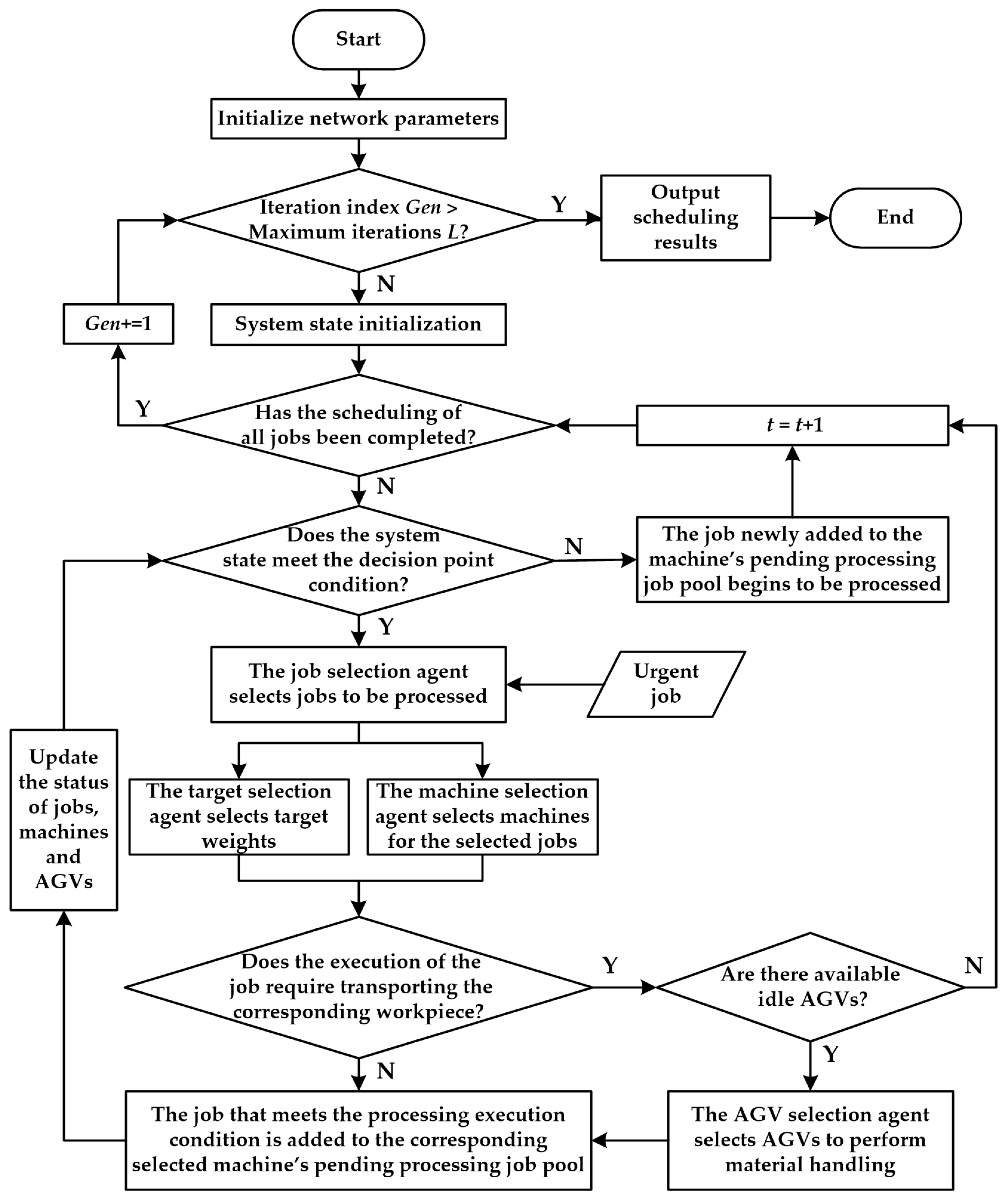
Urgent jobs usually require a manufacturing system to be able to respond quickly, so the event-driven strategy was adopted in this study to handle urgent job insertion events. The essence of scheduling problems is allocating limited resources to meet the job requirements within a reasonable time to achieve one or more objectives. Accordingly, emergency order insertions will bring about changes in the production status of the workshop, and these changes can be captured through the changes in the values of some of the feature variables utilized to monitor the operational status of manufacturing systems. Therefore, the strategy for handling urgent job insertions involves the following two parts:

(1)

Job pool update

When an urgent job is inserted at a random time, its process information will be recorded and the job will be added to the existing job pool following its insertion to wait for the assignment of scheduling objectives and machines.

(2)

State Feature Evaluation

To monitor the workshop production status, some feature variables, e.g., average job completion rate and the average expected processing time of the remaining operations, are designed, which also serve as a foundation for designing the state space and action space for various types of agents. After an urgent job is inserted, it will be merged into the initial job set to form a new job set. Correspondingly, the values of state feature variables will be updated based on the updated job information. By monitoring the state feature variables, the agent can perceive the occurrence of dynamic events to some extent and can be trained to handle them effectively.

4.2. Transformation of the ISPEA Problem

To solve the ISPEA problem using a MADL approach, no matter whether it is static or dynamic, it needs to be defined as a Markov game in the form of (N, S, A, T, γ, R), where N is the number of agents, S represents the state space, A represents the action space, T is the state transfer function, γ represents the discount factor for cumulative rewards, and R denotes the reward received by various agents after executing actions in state s and transitioning to state s’. Moreover, the concept of a decision point is proposed in this study. A decision point can be interpreted as the opportunity presented when idle jobs and idle machines that are capable of executing idle jobs coexist. To illustrate the key components of the Markov game, some parameter and variable symbols are also defined, as shown in

Table 2. Parameters and variables used to solve the ISPEA problem.

Symbol	Definition
eij	$\mathrm{Average} \mathrm{processing} \mathrm{EC} \mathrm{of} O_{ij}, e_{ij}={\displaystyle \frac{1}{N_{ij}}}{\displaystyle \sum _{\{k:O_{ij}\in N_k\}}\left(T_{ijk}^{\mathrm{M}}{P}_k^{\mathrm{M}}\right)}$
t	Decision point moment
Tij	$\mathrm{Average} \mathrm{processing} \mathrm{time} \mathrm{of} O_{ij}, T_{ij}={\displaystyle \frac{1}{N_{ij}}}{\displaystyle \sum _{\{k:O_{ij}\in N_k\}}{T}_{ijk}^{\mathrm{M}}}$
$U_h^t$	$\mathrm{Utilization} \mathrm{rate} \mathrm{of} \mathrm{AGV} h \mathrm{at} \mathrm{the} \mathrm{decision} \mathrm{point} \mathrm{time} t, U_h^t={\displaystyle \frac{1}{t}}{\displaystyle {\sum }_{i=1}^n{\displaystyle {\sum }_{j=1}^{x_i^t}\left[(C_{ij}^{\mathrm{A}}-S_{ij}^{\mathrm{A}})Z_{ijh}\right]}}$
$U_k^t$	$\mathrm{Utilization} \mathrm{rate} \mathrm{of} \mathrm{machine} k \mathrm{at} \mathrm{the} \mathrm{decision} \mathrm{point} \mathrm{time} t, U_k^t={\displaystyle \frac{1}{t}}{\displaystyle {\sum }_{i=1}^n{\displaystyle {\sum }_{j=1}^{x_i^t}\left(T_{ijk}^{\mathrm{M}}{X}_{ijk}\right)}}$
$V_h^t$	$\mathrm{The} \mathrm{machine} \mathrm{position} \mathrm{when} \mathrm{the} \mathrm{AGV} \mathrm{that} \mathrm{is} \mathrm{available} \mathrm{to} \mathrm{transport} \mathrm{a} \mathrm{workpiece} \mathrm{parks} \mathrm{at} \mathrm{the} \mathrm{decision} \mathrm{point} \mathrm{time} t, \mathrm{and} V_h^t\in [1,m]$
$x_i^t$	Number of completed operations of job i at the decision point time t

.

(1)

State space definition

The state space defines the set of all possible states that the agent can encounter in the environment and determines the information that is available to the agent for decision-making. In this study, the state representation designed to capture the information of the manufacturing system is mainly related to the current operational status of the manufacturing system, job conditions, and resource availability, as illustrated in

Table 3. State space.

Category	State Feature	Description
System state	$s_1={\displaystyle \frac{1}{n}}{\displaystyle {\sum }_{i=1}^n\left(x_i^t/l_i\right)}$	Average job completion rate
	$s_2=\sqrt{{\displaystyle \frac{1}{n}}{\displaystyle {\sum }_{i=1}^n{\left(x_i^t/l_i-s_1\right)}^2}}$	Standard deviation of job completion rate
	$s_3={\displaystyle \frac{1}{n}}{\displaystyle {\sum }_{i=1}^n{\displaystyle {\sum }_{j=x_i^t+1}^{l_i}{T}_{ij}}}$	Average expected processing time of the remaining job operations
	$s_4=\sqrt{{\displaystyle \frac{1}{n}}{\displaystyle {\sum }_{i=1}^n{\left({\displaystyle {\sum }_{j=x_i^t+1}^{l_i}{T}_{ij}}-s_3\right)}^2}}$	Standard deviation of the processing time of the remaining job operations
Job selection agent	$f_{11}={\displaystyle \frac{1}{n}}{\displaystyle {\sum }_{i=1}^n\left(x_i^t/l_i\right)}$	Average job completion rate
	$f_{12}=\sqrt{{\displaystyle \frac{1}{n}}{\displaystyle {\sum }_{i=1}^n{\left(x_i^t/l_i-f_{11}\right)}^2}}$	Standard deviation of job completion rate
	$f_{13}={\displaystyle \frac{1}{n}}{\displaystyle {\sum }_{i=1}^n{T}_{i\left(x_i^t+1\right)}}$	Average processing time of the next job operation
	$f_{14}=\sqrt{{\displaystyle \frac{1}{n}}{\displaystyle {\sum }_{i=1}^n{\left(T_{i\left(x_i^t+1\right)}-f_{13}\right)}^2}}$	Standard deviation of the processing time of the next job operation
	$f_{15}={\displaystyle \frac{1}{n}}{\displaystyle {\sum }_{i=1}^n{\displaystyle {\sum }_{j=x_i^t+1}^{l_i}{T}_{ij}}}$	Average expected processing time of the remaining job operations
	$f_{16}=\sqrt{{\displaystyle \frac{1}{n}}{\displaystyle {\sum }_{i=1}^n{\left({\displaystyle {\sum }_{j=x_i^t+1}^{l_i}{T}_{ij}}-f_{15}\right)}^2}}$	Standard deviation of the processing time of the remaining job operations
	$f_{17}={\displaystyle \frac{1}{n}}{\displaystyle {\sum }_{i=1}^n{e}_{i\left(x_i^t+1\right)}}$	Average processing EC of the next job operation
	$f_{18}=\sqrt{{\displaystyle \frac{1}{n}}{\displaystyle {\sum }_{i=1}^n{\left(e_{i\left(x_i^t+1\right)}-f_{17}\right)}^2}}$	Standard deviation of the processing EC of the next job operation
Machine selection agent	$f_{21}={\displaystyle \frac{1}{N_{ij}}}{\displaystyle \sum _{\{k:O_{ij}\in N_k\}}{U}_k^t}$	Average utilization rate of available machines
	$f_{22}=\sqrt{{\displaystyle \frac{1}{N_{ij}}}{{\displaystyle \sum _{\{k:O_{ij}\in N_k\}}\left(U_k^t-f_{21}\right)}}^2}$	Standard deviation of the utilization rate of available machines
	$f_{23}=\sqrt{{\displaystyle \frac{1}{N_{ij}}}{{\displaystyle \sum _{\{k:O_{ij}\in N_k\}}\left(T_{ijk}^{\mathrm{M}}{P}_k^{\mathrm{M}}-e_{ij}\right)}}^2}$	Standard deviation of the processing EC of available machines
	$f_{24}=\sqrt{{\displaystyle \frac{1}{N_{ij}}}{\displaystyle \sum _{\{k:O_{ij}\in N_k\}}{\left(T_{ijk}^{\mathrm{M}}-T_{ij}\right)}^2}}$	Standard deviation of the processing time of available machines
	$f_{25}=f_{24}/T_{ij}$	Distribution coefficient of the processing time
Target selection agent	$f_{31}=T_{ij}$	Average processing time of available machines
	$f_{32}=e_{ij}$	Average processing EC of available machines
	$f_{33}=\sqrt{{\displaystyle \frac{1}{N_{ij}}}{\displaystyle \sum _{\{k:O_{ij}\in N_k\}}{\left(T_{ijk}^{\mathrm{M}}{P}_k^{\mathrm{M}}-e_{ij}\right)}^2}}$	Standard deviation of the processing EC of available machines
	$f_{34}=\sqrt{{\displaystyle \frac{1}{N_{ij}}}{\displaystyle \sum _{\{k:O_{ij}\in N_k\}}{\left(T_{ijk}^{\mathrm{M}}-T_{ij}\right)}^2}}$	Standard deviation of the processing time of available machines
	$f_{35}=f_{33}/e_{ij}$	Distribution coefficient of processing EC
	$f_{36}=f_{34}/T_{ij}$	Distribution coefficient of processing time
AGV selection agent	$f_{41}={\displaystyle \frac{1}{q}}{\displaystyle {\sum }_{h=1}^q{U}_h^t}$	Average AGV utilization rate
	$f_{42}={\displaystyle \frac{1}{q}}{\displaystyle {\sum }_{h=1}^q{\displaystyle {\sum }_{i=1}^n{\displaystyle {\sum }_{j=1}^{x_i^t}\left[\left(C_{ij}^{\mathrm{A}}-S_{ij}^{\mathrm{A}}\right)P_h^{\mathrm{A}}{Z}_{ijh}\right]}}}$	Average AGV transport EC
	$f_{43}=\sqrt{{\displaystyle \frac{1}{q}}{\displaystyle {\sum }_{h=1}^q{\left(U_h^t-f_{41}\right)}^2}}$	Standard deviation of AGV utilization rate
	$f_{44}=\sqrt{{\displaystyle \frac{1}{q}}{\displaystyle {\sum }_{h=1}^q{\left[{\displaystyle {\sum }_{i=1}^n{\displaystyle {\sum }_{j=1}^{x_i^t}\left(C_{ij}^{\mathrm{A}}-S_{ij}^{\mathrm{A}}\right)P_h^{\mathrm{A}}{Z}_{ijh}-f_{42}}}\right]}^2}}$	Standard deviation of AGV transport EC
	$f_{45}=f_{43}/f_{41}$	Distribution coefficient of AGV utilization rate

.

(2)

Action space definition

The action space comprises the possible actions that the agent can take in a given state, which determine the agent’s ability to optimize the system performance and user experience. The action spaces of the four types of agents are different from each other, as displayed in

Table 4. Action space of the job selection agent.

Job Selection Rule	Description
EDD + LSO	Select the job with the highest urgency; if there are multiple jobs with the highest urgency, choose the one with the longest average processing time for the next operation.
EDD + SSO	Select the job with the highest urgency; if there are multiple jobs with the highest urgency, choose the one with the shortest average processing time for the next operation.
FIFO + LWKR	Select the job with the longest operation completion time; if there are multiple jobs with the longest completion time, choose the one with the shortest remaining processing time.
FIFO + MWKR	Select the job with the longest operation completion time; if there are multiple jobs with the longest completion time, choose the one with the longest remaining processing time.
LIFO + LWKR	Select the job with the shortest operation completion time; if there are multiple jobs with the shortest completion time, choose the one with the shortest remaining processing time.
LIFO + MWKR	Select the job with the shortest operation completion time; if there are multiple jobs with the shortest completion time, choose the one with the longest remaining processing time.
LOR + LWKR	Select the job with the highest processing progress; if there are multiple jobs with the highest processing progress, choose the one with the shortest remaining processing time.
LOR + MWKR	Select the job with the highest processing progress; if there are multiple jobs with the highest processing progress, choose the one with the longest remaining processing time.
LWKR + LSO	Select the job with the shortest remaining operation time; if there are multiple jobs with the shortest remaining operation time, choose the one with the longest average processing time for the next operation.
LWKR + SSO	Select the job with the shortest remaining operation time; if there are multiple jobs with the shortest remaining operation time, choose the one with the shortest average processing time for the next operation.
MOR + LWKR	Select the job with the lowest processing progress; if there are multiple jobs with the lowest processing progress, choose the one with the shortest remaining processing time.
MOR + MWKR	Select the job with the lowest processing progress; if there are multiple jobs with the lowest progress, choose the one with the longest remaining processing time.
MWKR + LSO	Select the job with the longest remaining operation time; if there are multiple jobs with the longest remaining operation time, choose the one with the longest average processing time for the next operation.
MWKR + SSO	Select the job with the longest remaining operation time; if there are multiple jobs with the longest remaining operation time, choose the one with shortest average processing time for the next operation.

,

Table 5. Action Space of the machine selection agent.

Machine Selection Rule	Description
Mrule1	Select the machine with the longest completion time for the last operation of the job at the decision point.
Mrule2	Select the machine with the shortest completion time for the last operation of the job at the decision point.
Mrule3	Select the machine with the lowest utilization rate at the decision point.
Mrule4	Select the machine with the highest utilization rate at the decision point.
Mrule5	Select the machine with the longest total idle time at the decision point.
Mrule6	Select the machine with the shortest total idle time at the decision point.
Mrule7	Select the machine that will result in the highest increase in the total production EC after completing the operation to be processed.
Mrule8	Select the machine that will result in the lowest increase in the total production EC after completing the operation to be processed.
Mrule9	Select the machine with the shortest processing time for the operation to be processed.
Mrule10	Select the machine with the longest processing time for the operation to be processed.
Mrule11	Select the machine with the lowest processing EC for the operation to be processed.
Mrule12	Select the machine with the highest processing EC for the operation to be processed.
Mrule13	Select the machine that will result in the lowest total production EC after completing the operation to be processed.
Mrule14	Select the machine that will result in the highest total production EC after completing the operation to be processed.

,

Table 6. Action space of the target selection agent (α-weight of C_max; β-weight of E_total).

Target Selection Rule	Description	Target Selection Rule	Description
Orule1	α = 1, β = 0	Orule6	α = 0.5, β = 0.5
Orule2	α = 0.9, β = 0.1	Orule7	α = 0.4, β = 0.6
Orule3	α = 0.8, β = 0.2	Orule8	α = 0.3, β = 0.7
Orule4	α = 0.7, β = 0.3	Orule9	α = 0.2, β = 0.8
Orule5	α = 0.6, β = 0.4	Orule10	α = 0.1, β = 0.9

and

Table 7. Action space of the AGV selection agent.

AGV Selection Rule	Description
Arule1	Select the earliest available AGV at the decision point.
Arule2	Select the latest available AGV at the decision point.
Arule3	Select the available AGV closest to the workpiece to be transported at the decision point.
Arule4	Select the available AGV farthest from the workpiece to be transported at the decision point.
Arule5	Select the AGV with the highest utilization rate at the decision point.
Arule6	Select the AGV with the lowest utilization rate at the decision point.

, and the scheduling process is achieved through collaborative efforts among these agents. Note that the composite action rules in Table 4 comprise simple action rules represented by abbreviations: EDD—earliest due date; FIFO—first in first out; LIFO—last in first out; LOR—least operation remaining; LSO—longest subsequent operation; LWKR—least work remaining; MOR—most operation remaining; MWKR—most work remaining; SSO—shortest subsequent operation.

In Table 5, some machine selection rules are not simply based on the known parameter information but require relatively complex processing to obtain the decision-making support information. For example, for Mrule5 and Mrule6, it is necessary to traverse all available idle machines for the upcoming operation of the selected job and extract all idle intervals for the available idle machines from time zero based on the information from the already executed operations. Then, a suitable machine can be selected after obtaining the total idle time of each available idle machine. Additionally, for Mrule7 and Mrule8, it is necessary to first obtain the idle time increment of each available idle machine k, which is the difference between the decision point time and the completion time of the last operation closest to the decision point time on machine k ($C_k^t$). Then, the EC increment ($\Delta E_{\mathrm{total}}^k$) is the sum of the processing EC for the upcoming operation and the idle EC increment, i.e., $\Delta E_{\mathrm{total}}^k=T_{ijk}^{\mathrm{M}}{P}_k^{\mathrm{M}}+(t-C_k^t)P_k^{\mathrm{I}}$, and the suitable machine will be selected by $\Delta E_{\mathrm{total}}^k$. Moreover, for Mrule13 and Mrule14, the total idle time of each available idle machine k will be updated to the sum of the known total idle intervals ($T_k^{\mathrm{I}}$) and the newly generated idle interval, and the total processing time of each available idle machine k will be updated to the sum of the processing time of the already processed operations ($T_k^{\mathrm{M}}$) and the processing time of the upcoming operation. Then, the total production EC of machine k ($E_{\mathrm{total}}^k$) will be updated, i.e., $E_{\mathrm{total}}^k=P_k^{\mathrm{M}}(T_k^{\mathrm{M}}+T_{ijk}^{\mathrm{M}})+P_k^{\mathrm{I}}\left[T_k^{\mathrm{I}}+(t-C_k^t)\right]$, and the available idle machine with the lowest/highest total production EC will be selected. In general, once a specific machine is chosen to execute the selected job, the values of decision variables X_ijk and $Y_{iji’j’k}$ can be directly determined.

Similarly, for Arule3 and Arule4 in Table 7, it is necessary to acquire all available idle AGVs at the decision point and obtain the corresponding location $V_h^t$ of each available idle AGV h. Then, the distances between each available idle AGV’s location and the transport job’s target machine can be compared, which are defined as the known parameter $T_{k{k}^{*}}^{\mathrm{A}}$ in Table 1, and the AGV with the minimum/maximum transport distance will be selected to execute the assigned transport job. Overall, the transport jobs needed in production are determined by the machine selected to execute each job. Once an AGV is assigned to execute a transport task at the decision point, the values of decision variables Z_ijh and $S_{ij}^{\mathrm{A}}$ can be directly acquired; then, the value of the decision variable $S_{ij}^{\mathrm{M}}$ can be indirectly obtained.

(3)

Reward function

The reward function plays a crucial role in guiding the agent’s learning process by providing feedback on the desirability of its actions, so its design should be closely related to the scheduling objectives. In this study, the reward function is defined as follows:

$$r=-\alpha {\displaystyle \frac{T_{ijk}^{\mathrm{M}}-\min \left\{T_{ijk}^{\mathrm{M}}\right\}}{\max \left\{T_{ijk}^{\mathrm{M}}\right\}-\min \left\{T_{ijk}^{\mathrm{M}}\right\}}}-{\displaystyle \frac{1}{2}}\beta ({\displaystyle \frac{T_{ijk}^{\mathrm{M}}{P}_k^{\mathrm{M}}-\min \left\{T_{ijk}^{\mathrm{M}}{P}_k^{\mathrm{M}}\right\}+E_{\mathrm{I}}-E_{{\mathrm{I}}^{-}}}{\max \left\{T_{ijk}^{\mathrm{M}}{P}_k^{\mathrm{M}}\right\}-\min \left\{T_{ijk}^{\mathrm{M}}{P}_k^{\mathrm{M}}\right\}}}+{\displaystyle \frac{T_{k{k}^{*}}^{\mathrm{A}}{P}_h^{\mathrm{A}}-\min \left\{T_{k{k}^{*}}^{\mathrm{A}}{P}_h^{\mathrm{A}}\right\}+E_{\mathrm{S}}-E_{{\mathrm{S}}^{-}}}{\max \left\{T_{k{k}^{*}}^{\mathrm{A}}{P}_h^{\mathrm{A}}\right\}-\min \left\{T_{k{k}^{*}}^{\mathrm{A}}{P}_h^{\mathrm{A}}\right\}}})$$

(20)

where $E_{{\mathrm{I}}^{-}}$ and $E_{{\mathrm{S}}^{-}}$ are the total standby EC of machines and AGVs, respectively, before the action selection is executed.

4.3. Agent Collaboration Process

Based on the dynamic event handling strategy and different types of agents designed, the process of various agents collaborating to solve the ISPEA problem is illustrated in Figure 1.

When the manufacturing system exits the decision point, for machines with newly added jobs in their pending processing job pools, the processing start time of these newly added jobs is related to whether material handling is needed. If transport assistance is not required, the starting time of processing the corresponding job will be the decision point time; otherwise, it will be the end time of the AGV transport process from the decision point time. Therefore, the values of the decision variables $S_{ij}^{\mathrm{A}}$ and $S_{ij}^{\mathrm{M}}$ can be determined using the judgment of the decision point.

4.4. QMIX Architecture

QMIX is a value-based MARL algorithm integrating the ideas of Actor–Critic and DQN algorithms, which adopts centralized learning and distributed execution strategies to train multiple agents. The centralized critic network receives the global state to guide the update of the actor network. Meanwhile, the DQN idea is employed to establish estimation and target networks for the critic network, and the time difference error TD_error is calculated to update the critic network.

QMIX utilizes a network to decompose the joint Q-value into a sophisticated nonlinear combination of the Q-values obtained by each agent according to its local observations, and the global and individual strategies are consistent. The standard QMIX architecture, as shown in Figure 2, consists of a mixing network, an agent network structure, and a set of hypernetworks. Each agent has its own network, which takes the current observation and the previous action $(o_t^a,u_{t-1}^a)$ as inputs and outputs an individual value function $Q_a({\tau }^a,u_t^a)$ at each time step. The weights and biases of the mixing network are produced by the hypernetworks. The hypernetworks take the current system state s_t as input and output a vector that is reshaped into an appropriately sized matrix to form the weights and biases of the mixing network. To guarantee the non-negativity of the mixing network weights, the hypernetwork is designed with a linear layer followed by an absolute value activation function. The intermediate layer biases are obtained through a linear layer, and the final biases are generated by a nonlinear two-layer hypernetwork using an ReLU activation function.

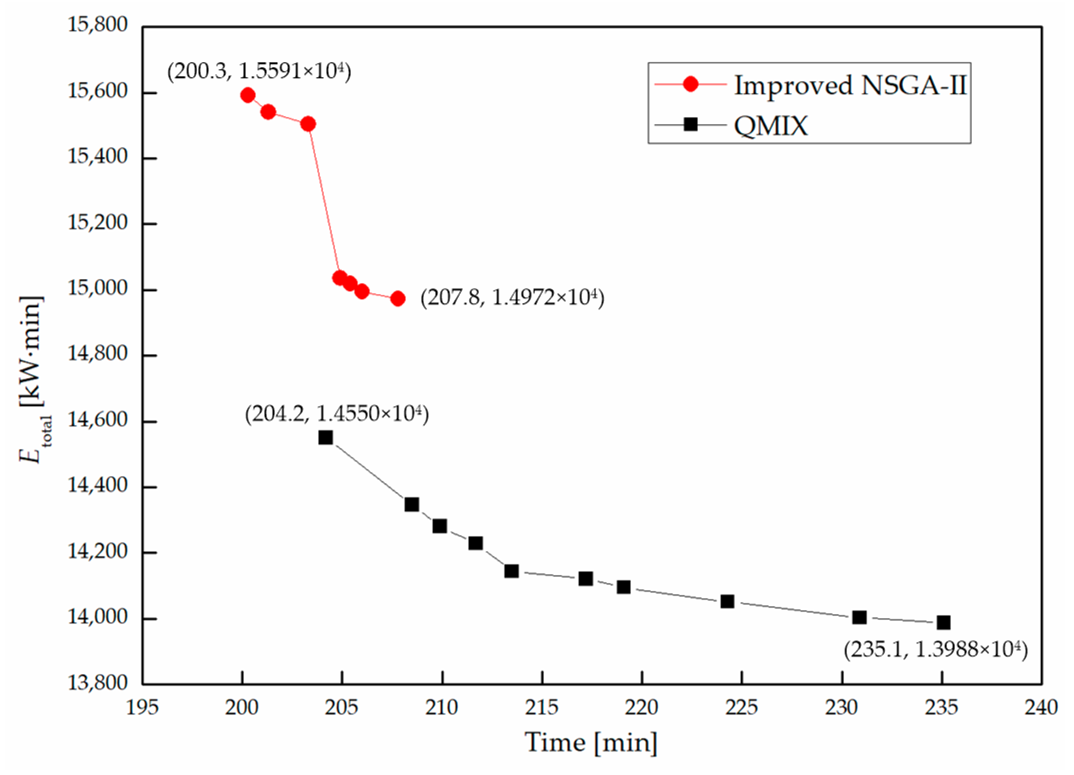
Note that the continuous empirical data generated by the agent–environment interaction in the RL process often show strong correlations, which can easily result in overfitting during training and affect the algorithm’s generalization ability. Additionally, the reward function incrementally shapes the agent’s strategy throughout the long-term learning process, affecting the balance between the agent’s interests and the group’s interests. To better achieve the collaborative optimization of various scheduling objectives and improve the algorithm optimization performance, the following three aspects of the classic QMIX are improved in this study:

(1)

Multi-Objective Solving Strategy

The current research on applying RL to address workshop scheduling problems seldom touches on the EC objective, and the related work usually transforms the scheduling problem into an SOP by assigning a specific weight to the EC objective. However, this approach restricts the range of searching for optimal solutions in the solution space. Considering that the Pareto solutions of an MOP are usually not unique, the designed target selection agent is integrated into the QMIX architecture, which can adjust the weights of the two optimization objectives of the ISPEA problem within a round according to the different decision environments, thereby expanding the search scope and effectively achieving multi-objective optimization solutions.

(2)

Reward Correction Strategy

RL relies on step-by-step immediate rewards that accumulate to generate the overall reward for a round. In unsupervised situations, if RL relies solely on reward signals, these signals are delayed, and it may take a long time to determine whether the current action is effective. Therefore, only relying on immediate rewards may result in a discrepancy between the actual scheduling results and the cumulative overall reward. Correspondingly, a reward correction strategy is formulated, which adds delayed rewards based on the objectives to correct the overall results at the end of a round.

The reward correction strategy integrates immediate rewards and delayed rewards to form a comprehensive reward function, ensuring the timely and correct utilization of reward signals. When designing the reward function, it is essential to strike a balance between immediate and delayed rewards to avoid overly pursuing short-term rewards while neglecting long-term benefits. Therefore, experiments are needed to adjust the weights of these rewards to find the most effective learning strategy.

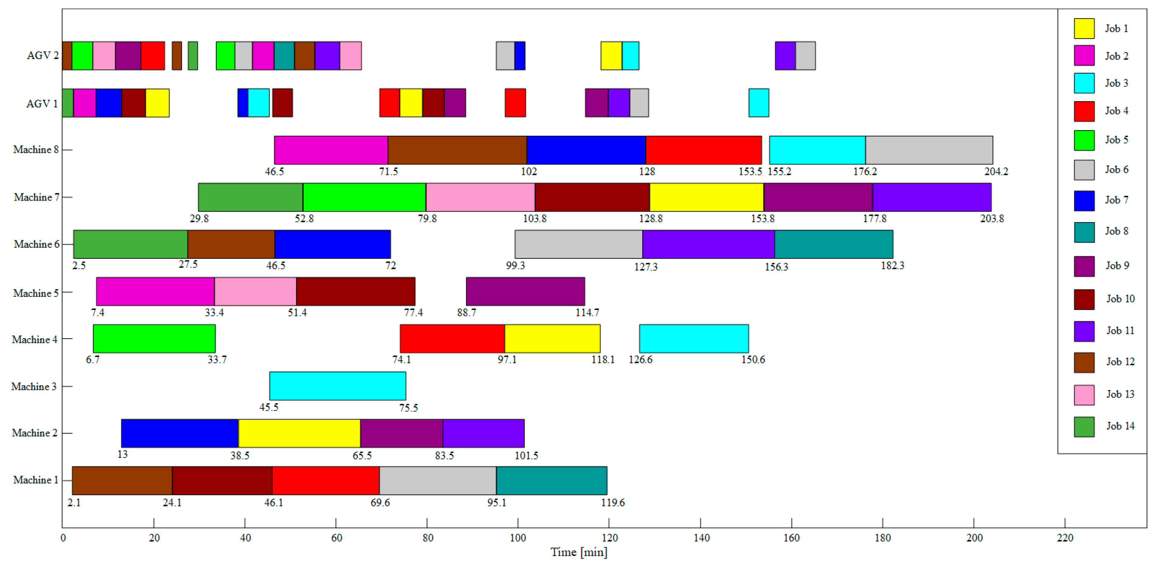
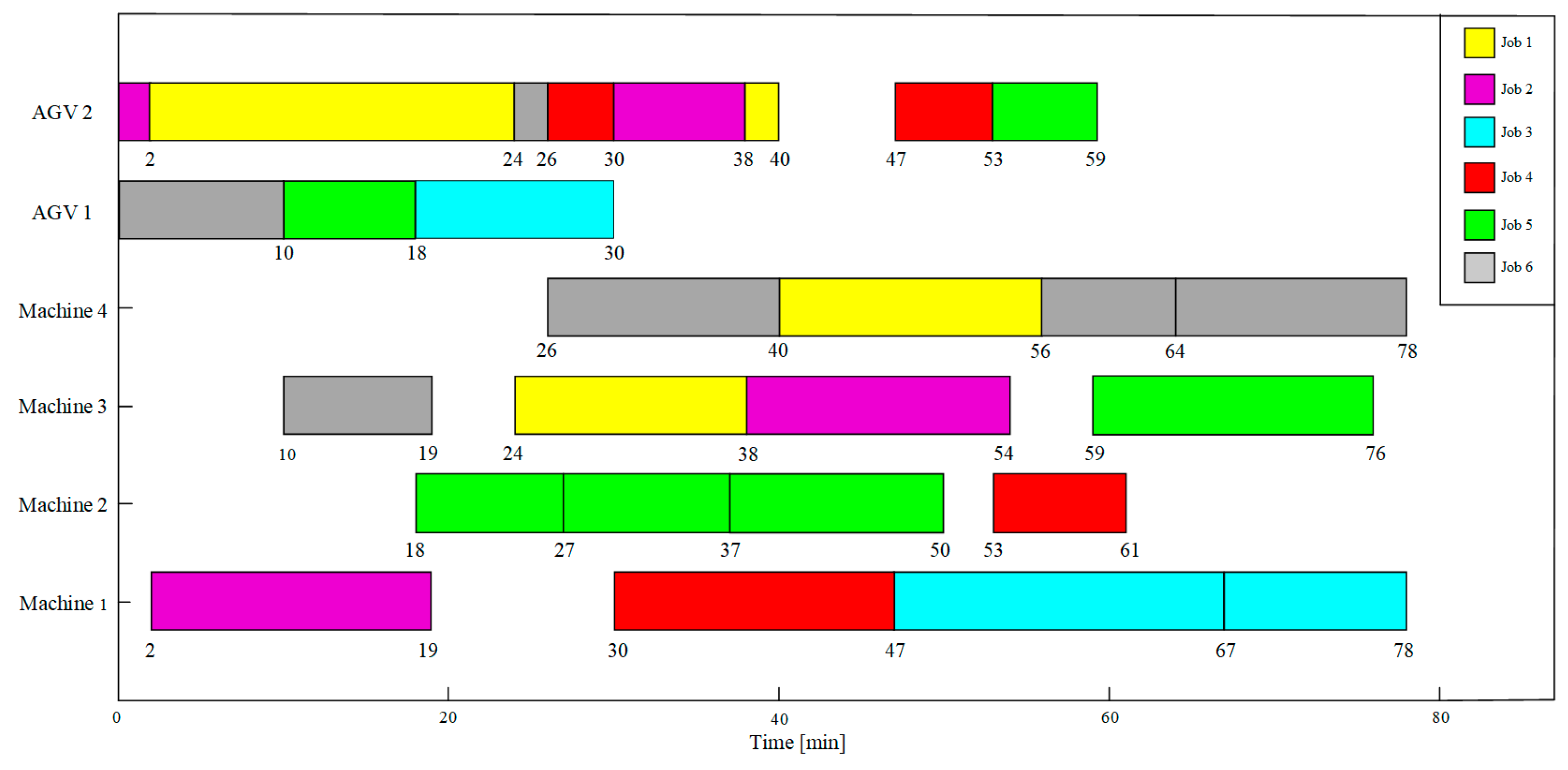
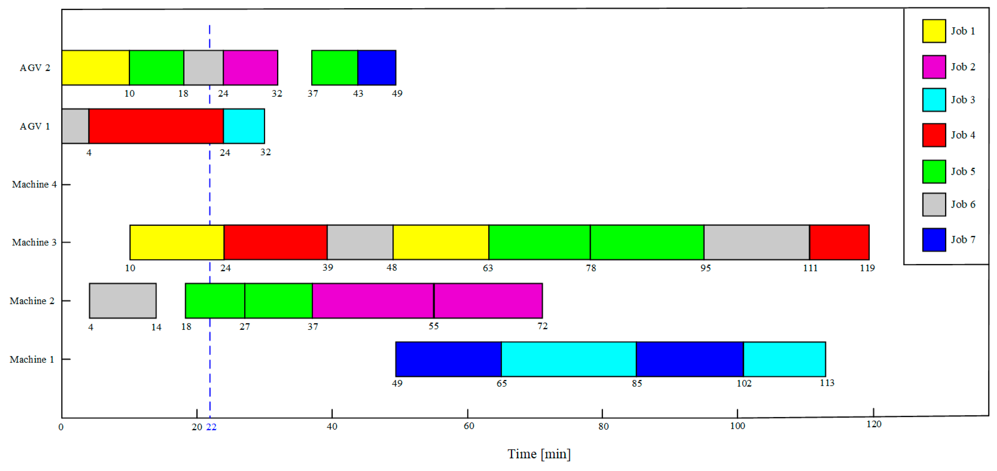
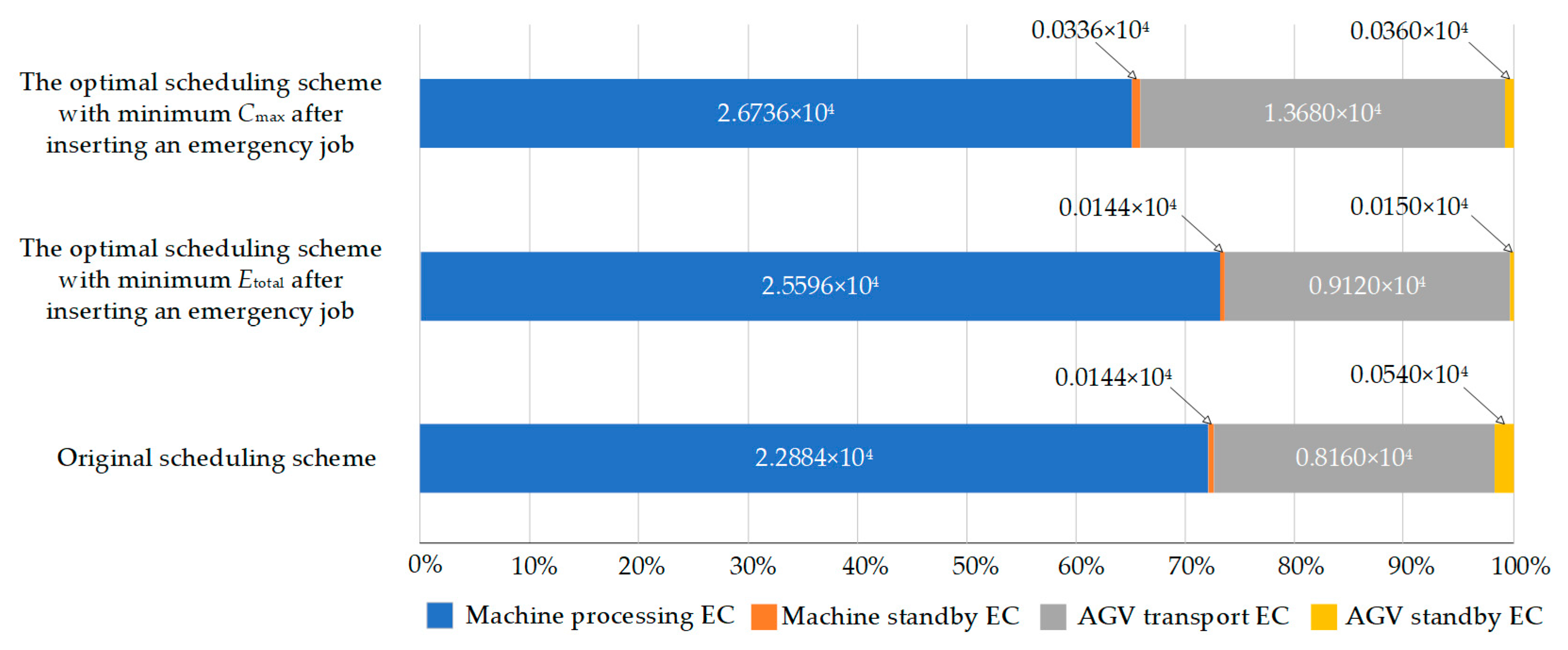
Combining this with the dynamic event handling strategy, when an urgent job is inserted, a delayed reward needs to be offered based on the difference between the completion time and delivery time of the inserted job, and the reward function represented by Formula (20) will be updated as follows:

$$r+=({\displaystyle \frac{T_{\mathrm{D}}-T_C}{T_{\mathrm{D}}}}-{\displaystyle \frac{C_{\max }}{C_{\max }^{*}}}-{\displaystyle \frac{E_{\mathrm{total}}}{E_{\mathrm{total}}^{*}}})$$

(21)

where $C_{\max }^{*}$ and $E_{\mathrm{total}}^{*}$ represent the theoretical minimum completion time and minimum total processing EC, respectively, and T_D is expressed as

$$T_{\mathrm{D}}=T_{\mathrm{J}}+{\displaystyle {\sum }_{j=1}^{l_{n+1}}{T}_{(n+1)j}}$$

(22)

(3)

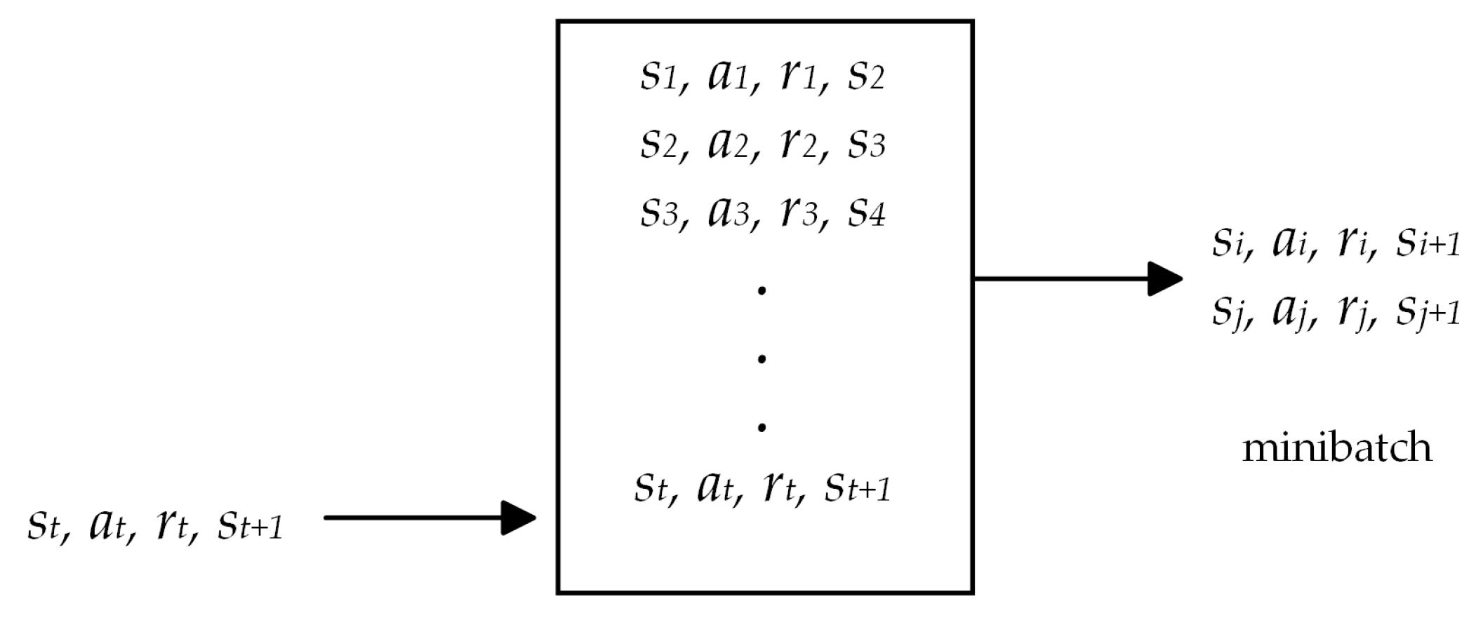
Prioritized Experience Replay Mechanism

Prioritized experience replay (PER) is a technique to enhance the DQN learning process. Classical experience replay stores interactions between the agent and the environment in a replay buffer. During the training process, a batch of transitions is randomly sampled from this buffer to update the network weights, as shown in Figure 3. This method treats all experiences equally, but their contribution to learning may not be the same in reality. Some experiences might be more valuable due to their rarity or the abundance of information they provide. Accordingly, PER tackles this issue by assigning a priority to each experience, enabling the more informative or crucial experiences to be sampled more frequently during training and improving the efficiency of the learning process.

The typical workflow of PER is as follows:

(1)

Priority assignment: Instead of randomly sampling experiences, priorities are determined based on the TD_error corresponding to each experience. The TD_error reflects the surprise of an experience, and a larger TD_error means the agent has more to learn from this experience.

(2)

Sampling: During network updates, experiences are sampled from the replay buffer according to their priority probabilities, and experiences with a higher TD_error are more likely to be selected.

(3)

Weight update: To guarantee the learning process remains unbiased, updates from the sampled experiences are weighted according to the reciprocal of their sampling probabilities, preventing some experiences from being oversampled and exerting too much influence on learning.

(4)

Stochastic sampling: To reduce the computational cost of calculating the precise TD_error for all experiences in the replay buffer, PER uses an approximate priority method.

To sum up, PER allows the agent to focus on the most beneficial experiences to improve training efficiency. Although PER introduces additional computational overhead due to the need to maintain priority and adjust updates, it can significantly enhance the performance of QMIX.

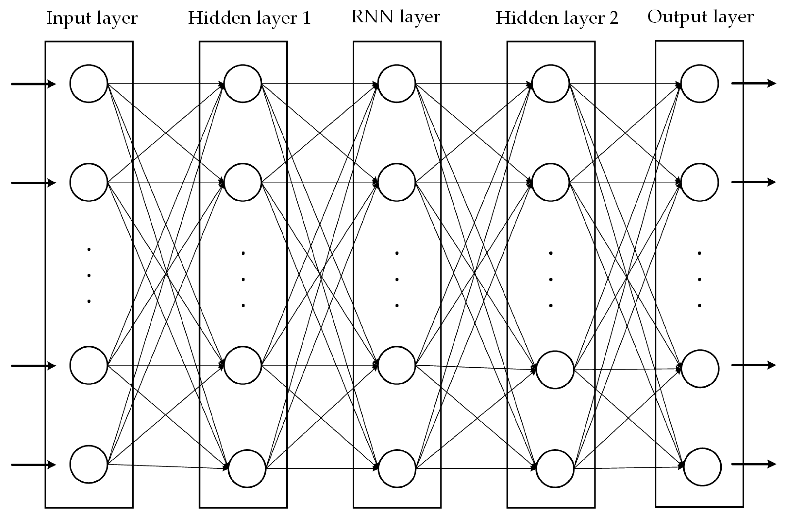
Within the improved QMIX algorithm framework, each agent is equipped with two sets of neural network models: an estimation network and a target network. These two types of networks have identical architectures but differ in their parameter update mechanisms. Specifically, the parameters of the estimation network are continuously updated with each training iteration. In contrast, the parameters of the target network are relatively static and only updated by copying the current parameters of the estimation network after a certain number of iterations. This design aims to reduce the correlation between Q-value estimates and Q-value targets, thereby enhancing the overall stability of the algorithm. The neural network architecture consists of an input layer, two hidden layers, a recurrent neural network (RNN) layer, and an output layer. The detailed network structure is illustrated in Figure 4. The specific configuration of the relevant parameters is provided in

Table 8. Estimation network and target network structure parameters.

Network Layer	Number of Nodes	Activation Function
Input layer of job selection agent/machine selection agent/target selection agent/AGV selection agent	22/19/16/14	/
Hidden layer 1	32	ReLU
RNN layer	32	ReLU
Hidden layer 2	32	ReLU
Output Layer	14	/

. Note that the number of nodes in the input layer varies according to the agent, and is equal to the sum of the elements of the current agent observation and the action taken in the previous time step. Each node in the output layer corresponds to the Q-value of each action in the current state.

4.5. QMIX Training and Execution

The improved QMIX comprises offline training and online execution, as depicted in Figure 5 and Figure 6, respectively, and aims to realize centralized training and decentralized execution. In the offline training phase, each agent takes actions based on its network, generating experiences that are stored. During network training, small batches of experiences are randomly selected from the experience pool. The Q-values for the actions chosen by each agent are computed, and the QMIX network structure combines these individual Q-values to obtain the overall Q-value. Then, TD_error is calculated, and the loss function can be obtained to guide the network training. In the online execution phase, the network parameters obtained from offline training are utilized for scheduling. Agents directly generate actions based on their observations, thereby completing the predefined scheduling tasks.

5. Case Study

To verify the effectiveness of the proposed method for solving dynamic ISPEA problems, the experimental study had two main aspects. Experiment 1 aims to comprehensively evaluate the performance of the QMIX method in this study based on the cases disclosed in the existing literature, and experiment 2 aims to test the ability of the proposed method to handle a dynamic ISPEA based on an actual production case originating from a customized furniture manufacturing workshop. The DQN in the QMIX architecture was implemented using the Python language and the Pytorch framework on a PC with an AMD Ryzen 5 5600H, with Radeon Graphics CPU@3.3 GHz, 16 GB RAM, and 64-bit Windows 11 OS.

The QMIX method’s overall performance is greatly impacted by the setting of basic parameters. The discount factor determines the extent to which future rewards influence current decisions. A higher discount factor (close to 1) indicates a greater focus on long-term rewards, while a lower discount factor (close to 0) emphasizes more immediate gains. Therefore, from the perspective of the essence of scheduling problems, this study initially selected a higher discount factor to allocate manufacturing resources reasonably over a longer time period to achieve maximum overall benefits. The learning rate determines the step size of each parameter update. While an overly low learning rate could cause the algorithm to converge slowly, an overly high learning rate could cause the algorithm to become unstable. Accordingly, to obtain high-quality solutions within a realistic calculation time, the learning rate should be set appropriately. The ε-greedy strategy was applied to balance exploration and exploitation, and the ε gradually decays at a certain rate as the training process progresses, based on its initial value. Its purpose is to allow for more exploration in the early stages of training to fully learn the environmental features, and gradually reduce this exploration in the later stages to focus more on utilizing the best strategies that have been learned. The capacity of the experience replay pool affects the training effectiveness of the model. An excessive capacity can increase the computational expense, while a low capacity may hinder the model from utilizing its historical experience for learning. Therefore, the capacity that is set for the experience replay pool should be able to maintain the diversity of the training process while ensuring model convergence and stability. The target network’s update frequency is mainly set to stabilize the learning process and improve training efficiency. The training parameter settings based on the existing applications of the QMIX [35] and our usage experience are shown in

Table 9. Training parameter settings.

Parameter	Value
Discount factor	0.96
Initial value of ε in ε-greedy strategy	1
Greedy strategy decay rate	0.002
Learning rate	0.001
Memory buffer capacity	100
Sample batch size	50
Target network update frequency	200
Maximum number of iterations	500

.

5.1. Experiment 1

To comprehensively evaluate the performance of the QMIX method used in this study, the FJSP benchmark case [36] and the shop floor layout proposed in [37] were utilized first, and the reward function was adjusted by ignoring the EC factors. Accordingly, the C_max obtained by the QMIX algorithm, DE algorithm [36], MAS algorithm [38], flexible multi-agent system (FMAS) algorithm [39], and multi-objective imperialist competitive algorithm (MICA) [40] is presented in

Table 10. Comparison of search results for examples at different scales.

	Method	DE [36]	MAS [38]	FMAS [39]	MICA [40]	QMIX
Example
EX11		96	130	111	98	88
EX12		82	98	87	79	69
EX13		84	109	91	83	74
EX14		103	168	128	109	94
EX21		100	143	128	106	98
EX22		76	86	88	73	83
EX23		86	98	102	92	89
EX24		106	169	131	112	110
EX31		99	142	114	95	99
EX32		85	114	99	82	86
EX33		86	103	102	81	85
EX34		110	167	128	119	110

.

Afterward, an FJSP with 14 jobs and 10 machines originating from a piston manufacturing workshop [41] was selected to further test the performance of the QMIX method. This workshop was equipped with two AGVs for material handling, and the specific job process information and resource EC characteristics can be referred to in [41]. When searching the optimal scheduling results with C_max and E_total as the optimization objectives, it should be noted that the E_total referenced in [41] includes the auxiliary energy consumed when maintaining the production environment (e.g., lighting, air conditioning, and heating), and the auxiliary EC was defined as the product of the auxiliary power factor and C_max. Then, the proposed QMIX method was run 20 times, and the Pareto solutions obtained are presented in

Table 11. Pareto solutions obtained by solving the case in [41].

	Pareto Solution No.	Cmax [min]	Etotal [kW·min]		Pareto Solution No.	Cmax [min]	Etotal [kW·min]
Optimization Objective				Optimization Objective
1		204.2	1.4550 × 104	6		217.2	1.4121 × 104
2		208.5	1.4346 × 104	7		219.1	1.4095 × 104
3		209.9	1.4280 × 104	8		224.3	1.4052 × 104
4		211.7	1.4229 × 104	9		230.9	1.4003 × 104
5		213.5	1.4144 × 104	10		235.1	1.3988 × 104

. The distribution of the Pareto solutions obtained by the QMIX method and the NSGA-II employed in [41] is presented in Figure 7, and the Gantt chart corresponding to the Pareto solution with the minimum E_total acquired by the QMIX method is depicted in Figure 8.

5.2. Experiment 2

Experiment 2 was related to a customized furniture manufacturing workshop, which belongs to the flexible job shop and is designed to meet the rapidly changing product demands of the furniture market. This workshop mainly produces six types of products, with four machines and two AGVs, and uses an energy management system, which enables the accurate collection of the daily electricity consumption data of machine tools by installing intelligent digital meters at each workstation. Furthermore, it implemented a working hour quota management system, which defines the expected time and resource consumption for each product during the production process. The job process information and machine EC characteristics for the six jobs planned for production in the workshop are displayed in

Table 12. Job information.

Job	Operation	Processing Time [min]
		Machine 1	Machine 2	Machine 3	Machine 4
1	$O_{11}$	16	15	14	-
	$O_{12}$	17	-	15	16
2	$O_{21}$	17	18	16	-
	$O_{22}$	-	17	16	15
3	$O_{31}$	20	-	19	19
	$O_{32}$	11	10	-	11
4	$O_{41}$	17	-	15	17
	$O_{42}$	-	8	8	10
5	$O_{51}$	8	9	10	-
	$O_{52}$	8	10	-	12
	$O_{53}$	-	13	15	13
	$O_{54}$	15	-	17	17
6	$O_{61}$	8	10	9	-
	$O_{62}$	-	16	15	14
	$O_{63}$	-	10	9	8
	$O_{64}$	15	-	16	14

and

Table 13. Machine power information.

Machine	1	2	3	4
$\mathrm{Average} \mathrm{processing} \mathrm{power} P_k^{\mathrm{M}}$ [kW]	2	1.6	1.8	2.4
Standby power $P_k^{\mathrm{I}}$ [kW]	0.5	0.6	0.3	0.4

, respectively. All raw materials and AGVs are initially in the workshop material distribution area, and all AGVs are on standby. The AGVs’ rated power is 2 kW, and the AGVs’ no-load power is 0.5 kW. Correspondingly, the time information of an AGV travelling between different machines and its initial position is listed in

Table 14. AGV transport time [min].

	To	Material Distribution Area	Machine 1	Machine 2	Machine 3	Machine 4
From
Material distribution area		0	2	4	10	12
Machine 1		12	0	2	8	10
Machine 2		10	12	0	6	8
Machine 3		4	6	8	0	2
Machine 4		2	4	6	12	0

.

For the above static ISPEA problem, which involved six jobs, four machines, and two AGVs, the proposed QMIX method was run 20 times, and the Pareto solutions obtained are presented in

Table 15. Pareto solutions obtained by solving the static ISPEA problem.

	Pareto Solution No.	1	2	3	4	5	6
Optimization Objectives
Cmax [min]		78	80	82	99	112	119
Etotal [kJ]		3.5844 × 104	3.3408 × 104	3.2616 × 104	3.2004 × 104	3.1734 × 104	3.1728 × 104

. Specifically, the Gantt charts of the scheduling scheme corresponding to the Pareto solution with the minimum C_max and E_total are depicted in Figure 9 and Figure 10, respectively.

Furthermore, to verify the effectiveness of the QMIX method in solving the dynamic ISPEA problem, an emergency job was randomly inserted in the time interval [20,40] when the workshop organized production according to the scheduling plan shown in Figure 10. Correspondingly, the index of the newly inserted job was marked as 7, and its process information is shown in

Table 16. Process information of the newly inserted job.

Operation No.	Processing Time [min]
	Machine 1	Machine 2	Machine 3	Machine 4
1	16	15	14	-
2	17	-	15	16

. The insertion time of the emergency job was the 22nd minute from time zero, which means the job pool should be updated, and the system running state variables also need to be updated accordingly after the 22nd minute. From the perspective of maintaining energy-efficient production after inserting the emergency job, the Gantt chart of the optimal scheduling scheme with the minimum E_total obtained by employing the QMIX method is depicted in Figure 11, and the specific values of optimization objectives E_total and C_max are 3.5010 × 10⁴ kJ and 80 min, respectively. Considering that urgent orders generally require prompt delivery, the optimal scheduling scheme with the minimum C_max was also searched, and the corresponding Gantt chart is displayed in Figure 12.

5.3. Discussion

In Experiment 1, from the perspective of the search results of the optimal solutions presented in Figure 9, the QMIX method outperforms the MAS and FMAS algorithms in all examples, outperforms the MICA in 66.67% of examples, and is not inferior to the DE algorithm in 58.33% of the examples. Moreover, according to Figure 7, although the optimal solutions obtained by the QMIX method are not better than those obtained by the improved NSGA-II on the optimization objective of C_max, the QMIX obtains better solutions for the optimization objective of E_total, which extends the boundary of the original Pareto front. Comparing the Pareto solutions with the minimum E_total, the E_total obtained by the improved NSGA-II was further optimized and decreased by 6.5%. Therefore, the QMIX method utilized in this study can be accepted for solving static ISPEA problems, especially in scenarios with energy-efficient production requirements. It should also be noted that heuristic and meta-heuristic algorithms require fewer computational resources and converge quickly for small-scale scheduling problems. Although the QMIX method finds better optimal solutions than the DE and MICA algorithms for small-scale scheduling problems, the QMIX training process is rather time-consuming and highly computationally demanding. Accordingly, the advantages of the traditional methods cannot be entirely disregarded in practical applications, and it is necessary to choose an appropriate method based on the problem scenario.

Since dynamic scheduling problems can be transformed into static scheduling problems for solutions, the QMIX method integrating the designed dynamic event handling strategy is also suitable for solving dynamic ISPEA problems. When an emergency job is added, its execution will inevitably use processing and transport resources. Due to the need to minimize the impact on the original scheduling plan when executing dynamic scheduling, it is necessary to improve resource utilization as much as possible, such as minimizing standby periods, making full use of energy-efficient machines, and reducing the frequency of workpiece handling. As shown in Figure 10, before inserting an emergency job, machines 2 and 3 are relatively busy, while machine 4 is idle. After adding a job, it can be found that the processing time for each operation of the new job on machine 1 is longer than on other alternative machines, and the average processing power of machine 1 is higher than that of machines 2 and 3. However, choosing machine 1 to process the newly inserted job can significantly reduce AGV transport EC. Therefore, as shown in Figure 11, all operations of the newly inserted job were arranged on machine 1 for processing. Although E_total increased by 10.34%, C_max remained unchanged.

Furthermore, the EC corresponding to various optimal scheduling schemes after inserting an emergency job was decomposed. As shown in Figure 13, the machine EC accounts for the majority of the total EC required to complete this batch of jobs. In terms of E_total, the total machine EC grew to fulfill demands of the emergency job, but the total machine standby EC remained unchanged through reasonable scheduling. Meanwhile, the total AGV EC increased by 6.55%, mostly due to an increase in AGV transport EC. Despite the similar power characteristics of machine 1 and the AGV, the processing time for the emergency job on machine 1 is much longer than its related transport time, resulting in a much greater increase in machine EC than AGV EC. In contrast, in terms of C_max, both total machine EC and total AGV EC increased. Specifically, the increase in AGV EC was greater, which was attributed to the increase in AGV transport activities. To shorten the job completion time, high-power machine 4 was put into use. Meanwhile, the increase in AGV transport activities increased the probability of machine tools waiting for jobs, leading to an increase in machine standby EC. In order to minimize the makespan, it is necessary to fully utilize all manufacturing resources and allocate workload reasonably. However, it should also be noted that the different equipment power characteristics and activity durations may lead to a sharp increase in E_total. As revealed in Figure 12, the previously idle machine 4 was assigned job operations, and the workload of machines 2 and 3 was reduced. Although C_max decreased by 32.77%, approaching the best C_max obtained before the insertion of the job, E_total increased by 29.57%.

Hence, the adjustment of the scheduling scheme for the newly inserted job has a certain value in practical applications, and the QMIX method is also effective in solving dynamic ISPEA problems.

6. Conclusions

At present, the manufacturing industry is accelerating its transformation and development toward greenization and intelligence. This paper takes flexible job shops as the research object, considers the impact of logistics factors and emergency order insertions in the workshop production process, and conducts dynamic ISPEA research with makespan and total production EC as the optimization objectives. Further, combined with the designed event handling strategy, the representative MARL algorithm QMIX is improved by integrating a multi-objective solving strategy, a reward correction strategy, and a prioritized experience replay mechanism to address the dynamic ISPEA problem, and its feasibility and effectiveness are verified through experimental research. The presented work also indicates that the ISPEA can optimize the makespan and total production EC simultaneously by selecting suitable machines and AGVs for jobs and rationally arranging the processing sequence of the operations allocated to each machine and the transport sequence of the job-related workpieces allocated to each AGV.

The introduction of MARL to address the complex decision-making problems in dynamic ISPEA can improve the flexibility and adaptability of the decision-making process. Through the cooperation of various agents, manufacturing systems can handle complex jobs and adapt to dynamic environments more efficiently. Correspondingly, the proposed model and method provide an effective solution for manufacturing enterprises with high levels of automation and intelligence (e.g., automobile and aerospace manufacturers) to achieve energy-efficient production, especially in flexible job shops that require the efficient utilization of both processing and logistics equipment. However, the potential limitations of this study should also be noted. This study only focuses on responses to emergency order insertions, but there are a variety of dynamic events in the workshop. Whether the proposed dynamic scheduling method can be adjusted to handle other types of dynamic events still needs exploration and demonstration. The DRL method applied in this study has long training times and requires a significant amount of computational resources for training in high-dimensional state spaces or spaces with frequent dynamic disturbances. Therefore, its advantages in solving large-scale scheduling problems are not prominent, and there is still room for improvement. Moreover, the operating characteristics of all machines and AGVs, such as the power parameters and operation times of the job processes, are assumed to be known and fixed in this study. In actual production environments, these parameters may alter due to equipment aging or changes in working conditions, affecting the applicability and stability of the scheduling schemes. Furthermore, this study only investigates two scheduling optimization objectives, which may not fully reflect the actual scheduling requirements in complex production situations.

Therefore, to fully utilize the latest AI technology and explore the energy-saving potential of workshops from the perspective of the manufacturing system level, future research will focus on (1) improving the DRL method applied in this study and enhancing its generality; (2) considering more types of dynamic events and introducing more optimization objectives; and (3) considering the impact of AGV path planning on developing energy-efficient scheduling schemes.

References

1. Lee, S.; Do Chung, B.; Jeon, H.W.; Chang, J. A dynamic control approach for energy-efficient production scheduling on a single machine under time-varying electricity pricing. J. Clean. Prod. 2017, 165, 552–563. [Google Scholar] [CrossRef]
2. Fernandes, J.M.R.C.; Homayouni, S.M.; Fontes, D.B.M.M. Energy-efficient scheduling in job shop manufacturing systems: A literature review. Sustainability 2022, 14, 6264. [Google Scholar] [CrossRef]
3. Missaoui, A.; Ozturk, C.; O’Sullivan, B.; Garraffa, M. Energy efficient manufacturing scheduling: A systematic literature review. arXiv 2023, arXiv:2308.13585. [Google Scholar]
4. Lei, D.; Zheng, Y.; Guo, X. A shuffled frog-leaping algorithm for flexible job shop scheduling with the consideration of energy consumption. Int. J. Prod. Res. 2017, 55, 3126–3140. [Google Scholar] [CrossRef]
5. Li, K.; Lin, B. Impact of energy conservation policies on the green productivity in China’s manufacturing sector: Evidence from a three-stage DEA model. Appl. Energy 2016, 168, 351–363. [Google Scholar] [CrossRef]
6. Zhang, L.; Feng, Y.; Xiao, Q.; Xu, Y.; Li, D.; Yang, D.; Yang, Z. Deep reinforcement learning for dynamic flexible job shop scheduling problem considering variable processing times. J. Manuf. Syst. 2023, 71, 257–273. [Google Scholar] [CrossRef]
7. Han, X.; Cheng, W.; Meng, L.; Zhang, B.; Gao, K.; Zhang, C.; Duan, P. A dual population collaborative genetic algorithm for solving flexible job shop scheduling problem with AGV. Swarm Evol. Comput. 2024, 86, 101538. [Google Scholar] [CrossRef]
8. Meng, L.; Zhang, B.; Gao, K.; Duan, P. An MILP model for energy-conscious flexible job shop problem with transportation and sequence-dependent setup times. Sustainability 2023, 15, 776. [Google Scholar] [CrossRef]
9. Kayhan, B.M.Z. Reinforcement Learning Based Solution Approaches to Static and Dynamic Machine Scheduling Problems. Ph.D. Thesis, Dokuz Eylul University, Izmir, Turkey, 2022. [Google Scholar]
10. Li, R.; Gong, W.; Lu, C.; Wang, L. A learning-based memetic algorithm for energy-efficient flexible job-shop scheduling with type-2 fuzzy processing time. IEEE Trans. Evol. Comput. 2023, 27, 610–620. [Google Scholar] [CrossRef]
11. Zhang, H.; Xu, G.; Pan, R.; Ge, H. A novel heuristic method for the energy-efficient flexible job-shop scheduling problem with sequence-dependent set-up and transportation time. Eng. Optim. 2022, 54, 1646–1667. [Google Scholar] [CrossRef]
12. Luo, S.; Zhang, L.; Fan, Y. Energy-efficient scheduling for multi-objective flexible job shops with variable processing speeds by grey wolf optimization. J. Clean. Prod. 2019, 234, 1365–1384. [Google Scholar] [CrossRef]
13. Zhang, Z.; Wu, L.; Peng, T.; Jia, S. An improved scheduling approach for minimizing total energy consumption and makespan in a flexible job shop environment. Sustainability 2019, 11, 179. [Google Scholar] [CrossRef]
14. Wu, X.; Shen, X.; Li, C. The flexible job-shop scheduling problem considering deterioration effect and energy consumption simultaneously. Comput. Ind. Eng. 2019, 135, 1004–1024. [Google Scholar] [CrossRef]
15. Liu, L.; Song, H.; Jiang, T.; Deng, G.; Gong, Q. Modified biology migration algorithm for dual-resource energy-saving flexible job shop scheduling problem. Comput. Integr. Manuf. Syst. 2024, 30, 3125–3141. [Google Scholar] [CrossRef]
16. Zhang, L.; Tang, Q.; Wu, Z.; Wang, F. Mathematical modeling and evolutionary generation of rule sets for energy-efficient flexible job shops. Energy 2017, 138, 210–227. [Google Scholar] [CrossRef]
17. Rakovitis, N.; Li, D.; Zhang, N.; Li, J.; Zhang, L.; Xiao, X. Novel approach to energy-efficient flexible job-shop scheduling problems. Energy 2022, 238, 121773. [Google Scholar] [CrossRef]
18. Zhang, Y.; Wang, J.; Liu, Y. Game theory based real-time multi-objective flexible job shop scheduling considering environmental impact. J. Clean. Prod. 2017, 167, 665–679. [Google Scholar] [CrossRef]
19. Zhou, G.; Chen, Z.; Zhang, C.; Chang, F. An adaptive ensemble deep forest based dynamic scheduling strategy for low carbon flexible job shop under recessive disturbance. J. Clean. Prod. 2022, 337, 130541. [Google Scholar] [CrossRef]
20. Li, X.; Huang, J.; Li, J.; Li, Y.; Gao, L. Research and development trend of intelligent shop dynamic scheduling. Sci. Sin. (Technol. ) 2023, 53, 1016–1030. [Google Scholar] [CrossRef]
21. Bouazza, W.; Sallez, Y.; Beldjilali, B. A distributed approach solving partially flexible job-shop scheduling problem with a Q-learning effect. IFAC-Pap. OnLine 2017, 50, 15890–15895. [Google Scholar] [CrossRef]
22. Liu, R.; Piplani, R.; Toro, C. Deep reinforcement learning for dynamic scheduling of a flexible job shop. Int. J. Prod. Res. 2022, 60, 4049–4069. [Google Scholar] [CrossRef]
23. Zhou, L.; Zhang, L.; Horn, B.K.P. Deep reinforcement learning-based dynamic scheduling in smart manufacturing. Procedia CIRP 2020, 93, 383–388. [Google Scholar] [CrossRef]
24. Zhao, M.; Li, X.; Gao, L.; Wang, L.; Xiao, M. An improved Q-learning based rescheduling method for flexible job-shops with machine failures. In Proceedings of the 2019 IEEE 15th International Conference on Automation Science and Engineering (CASE 2019), Vancouver, BC, Canada, 22–26 August 2019; pp. 331–337. [Google Scholar]
25. Zhang, M.; Lu, Y.; Hu, Y.; Amaitik, N.; Xu, Y. Dynamic scheduling method for job-shop manufacturing systems by deep reinforcement learning with proximal policy optimization. Sustainability 2022, 14, 5177. [Google Scholar] [CrossRef]
26. Shahrabi, J.; Adibi, M.A.; Mahootchi, M. A reinforcement learning approach to parameter estimation in dynamic job shop scheduling. Comput. Ind. Eng. 2017, 110, 75–82. [Google Scholar] [CrossRef]
27. Li, K.; Deng, Q.; Zhang, L.; Fan, Q.; Gong, G.; Ding, S. An effective MCTS-based algorithm for minimizing makespan in dynamic flexible job shop scheduling problem. Comput. Ind. Eng. 2021, 155, 107211. [Google Scholar] [CrossRef]
28. Zhang, Y.; Zhu, H.; Tang, D.; Zhou, T.; Gui, Y. Dynamic job shop scheduling based on deep reinforcement learning for multi-agent manufacturing systems. Robot. Comput. -Integr. Manuf. 2022, 78, 102412. [Google Scholar] [CrossRef]
29. Gnanavel Babu, A.; Jerald, J.; Noorul Haq, A.; Muthu Luxmi, V.; Vigneswaralu, T.P. Scheduling of machines and automated guided vehicles in FMS using differential evolution. Int. J. Prod. Res. 2010, 48, 4683–4699. [Google Scholar] [CrossRef]
30. Zhong, H.; Peng, C.; Liao, Y.; Li, X. Combined rules based optimization for AGV joint scheduling in job shop. Manuf. Technol. Mach. Tool 2022, 11, 183–192. [Google Scholar] [CrossRef]
31. Li, Y.; Gu, W.; Yuan, M.; Tang, Y. Real-time data-driven dynamic scheduling for flexible job shop with insufficient transportation resources using hybrid deep Q network. Robot. Comput. -Integr. Manuf. 2022, 74, 102283. [Google Scholar] [CrossRef]
32. Yuan, M.; Zheng, L.; Huang, H.; Zhou, K.; Pei, F.; Gu, W. Research on flexible job shop scheduling problem with AGV using double DQN. J. Intell. Manuf. 2023. [Google Scholar] [CrossRef]
33. Sun, A.; Lei, Q.; Song, Y.; Yang, Y. Deep reinforcement learning for solving the joint scheduling problem of machines and AGVs in job shop. Control. Decis. 2024, 39, 253–262. [Google Scholar] [CrossRef]
34. Chakraborty, U.J. Computational Intelligence in Flow Shop and Job Shop Scheduling; Springer: Berlin/Heidelberg, Germany, 2009. [Google Scholar]
35. Rashid, T.; Samvelyan, M.; De Witt, C.S.; Farquhar, G.; Foerster, J.; Whiteson, S. QMIX: Monotonic value function factorisation for deep multi-agent reinforcement Learning. In Proceedings of the 35th International Conference on Machine Learning, Stockholm, Sweden, 10–15 July 2018; pp. 6846–6859. [Google Scholar]
36. Kumar, M.V.S.; Janardhana, R.; Rao, C.S.P. Simultaneous scheduling of machines and vehicles in an FMS environment with alternative routing. Int. J. Adv. Manuf. Technol. 2011, 53, 339–351. [Google Scholar] [CrossRef]
37. Bilge, Ü.; Ulusoy, G. A time window approach to simultaneous scheduling of machines and material handling system in an FMS. Oper. Res. 1995, 43, 911–1070. [Google Scholar] [CrossRef]
38. Erol, R.; Sahin, C.; Baykasoglu, A.; Kaplanoglu, V. A multi-agent based approach to dynamic scheduling of machines and automated guided vehicles in manufacturing systems. Appl. Soft Comput. 2012, 12, 1720–1732. [Google Scholar] [CrossRef]
39. Sahin, C.; Demirtas, M.; Erol, R.; Baykasoğlu, A.; Kaplanoğlu, V. A multi-agent based approach to dynamic scheduling with flexible processing capabilities. J. Intell. Manuf. 2017, 28, 1827–1845. [Google Scholar] [CrossRef]
40. Wang, H. Research on the Joint Scheduling Methon of Green Flexible Job Shop Machine and AGV. Master’s Thesis, Yangzhou University, Yangzhou, China, 2022. [Google Scholar]
41. Li, K. Research on the Integrated Scheduling Method of Flexible Job Shop Machines and AGVs. Master’ Thesis, Xi’an University of Technology, Xi’an, China, 2023. [Google Scholar]
Figure 1. Flowchart of the agent collaboration process.
Processes 12 02423 g001
Figure 2. Classic QMIX architecture diagram.
Processes 12 02423 g002
Figure 3. Experience replay mechanism.
Processes 12 02423 g003
Figure 4. Schematic diagram of the agent neural network structure.
Processes 12 02423 g004
Figure 5. QMIX offline training process.
Processes 12 02423 g005
Figure 6. QMIX online execution process.
Processes 12 02423 g006
Figure 7. Comparison of Pareto solution distributions.
Processes 12 02423 g007
Figure 8. Gantt chart corresponding to the Pareto solution with minimum Cmax (Cmax = 204.2 min, Etotal = 1.4550 × 10⁴ kW·min).
Processes 12 02423 g008
Figure 9. Gantt chart of the optimal scheduling scheme with the minimum Cmax (Cmax = 78 min, Etotal = 3.5844 × 10⁴ kJ).
Processes 12 02423 g009
Figure 10. Gantt chart of the optimal scheduling scheme with the minimum Etotal (Cmax = 119 min, Etotal = 3.1728 × 10⁴ kJ).
Processes 12 02423 g010
Figure 11. Gantt chart of the optimal scheduling scheme with minimum Etotal after inserting an emergency job (Cmax = 119 min, Etotal = 3.5010 × 10⁴ kJ).
Processes 12 02423 g011
Figure 12. Gantt chart of the optimal scheduling scheme with minimum Cmax after inserting an emergency job (Cmax = 80 min, Etotal = 4.1112 × 10⁴ kJ).
Processes 12 02423 g012
Figure 13. Decomposition of energy consumption corresponding to various optimal scheduling schemes.
Processes 12 02423 g013