Refracturing Time Optimization Considering the Effect of Induced Stress by Pressure Depletion in the Shale Reservoir

Abstract

Refracturing is an important technology for tapping remaining oil and gas areas and enhancing recovery in old oilfields. However, a complete and detailed refracturing timing optimization scheme has not yet been proposed. In this paper, based on the finite volume method and the embedded discrete fracture model, a new coupled fluid flow/geomechanics pore-elastic-fractured reservoir model is developed. The COMSOL 3.5 commercial software was used to verify the accuracy of our model, and by studying the influence of matrix permeability, initial stress difference, cluster spacing, and fracture half-length on the orientation of maximum horizontal stress, a timing optimization method for refracturing is proposed. The results of this paper show that the principle of optimizing the refracturing timing is to avoid the time window where the percentage of Type I (Type I indicates that stress inversion has occurred, $0^{\circ }\le \alpha \le {20}^{\circ }$; Type II indicates that the turning degree is strong, ${20}^{\circ }<\alpha \le {70}^{\circ }$; and Type III indicates less stress reorientation, ${70}^{\circ }<\alpha \le {90}^{\circ }$) stress reorientation area is relatively large, so that the fractures can extend perpendicular to the horizontal wellbore. At the same time, the simulation results show that with the increase in production time, the percentage of Type I and Type II increases first and then decreases, while the percentage of Type III decreases first and then increases. When the reservoir permeability, stress difference, and cluster spacing are larger, the two types of refracturing measures can be implemented earlier. But, with the increase in fracture half-length, the timing of refracturing Method I is earlier, and the timing of refracturing Method II is later. The research results of this paper are of great significance to the perfection of the refracturing theory and the optimization of refracturing design.

1. Introduction

Currently, hydraulic fracturing is the main method for enhancing oil recovery in major oil and gas fields. Particularly for unconventional reservoirs, a long horizontal stage with multistage and multi-cluster fracturing technology has achieved suitable development results [1,2,3,4,5]. However, as development entered the middle and late stages, the first fracture conductivity and nearby formation permeability gradually decreased owing to the influence of wax and scale formation, microparticle migration, and fracture closure, leading to a substantial decline in oil and gas productivity [6,7,8,9]. To relieve reservoir damage and improve reservoir recovery, refracturing technology for old wells has become an important way to exploit the potential of the remaining oil areas in old wells [10,11]. Refracturing refers to the refracturing of a well that has already been fractured once or more. Owing to different interpretations of repeated fracturing measures, the main refracturing methods include reopening the original fractures (keeping the first fracture open while the fracture does not expand), fracturing the original fractures and expanding them, and fracturing them after temporary plugging. In the Daqing, Changqing oil fields, Weiyuan, and Changning shale gas blocks in Sichuan Province, the refracturing technology has achieved remarkable economic benefits.

As early as the 1950s and the 1960s, researchers began conducting laboratory studies and field experiments on refracturing. However, owing to the extensive knowledge, comprehensive research methods, and difficult numerical simulations involved in refracturing, a set of scientific and systematic theoretical guidance methods have not yet been developed, resulting in many refracturing wells that have not achieved ideal results [12,13,14,15]. In the 1980s and the 1990s, the United States made refracturing an important topic, focusing on key research topics, such as refracturing mechanisms, materials, and design. Elbel et al. [16] verified for the first time that the initial fracturing of oil and gas wells will change the pressure gradient around the fractures, resulting in changes in the stress field of the reservoir. For reservoirs with small stress differences, the induced stress field can even cause a 90° reversal of the principal stress direction. Chevron Petroleum Technology also verified the turning process of hydraulic fractures during refracturing through on-site experiments in the Lost Hills Oil Field. Based on the elastic mechanics of porous media, Wright et al. [17] (1995) explained the internal mechanism of stress field changes induced by a reduction in pore pressure from the perspective of reservoir compaction and fracture slip.

Owing to the slow development of numerical simulation technology, early studies have mainly focused on theoretical analyses and experimental research. Since the early 20th century, research on the mechanisms of refracturing has entered a stage of rapid development. Gupta et al. [18] believed that the variation in the stress field is related to reservoir development and proposed that the smaller the horizontal principal stress difference in a reservoir, the more conducive it is to stress inversion. Roussel and Sharma [19] calculated the degree of stress redirection around fractured production and injection wells and analyzed its impact on refracturing operations. Roussel et al. [20] demonstrated the stress reversal phenomenon by studying the evolution of stress fields around infill wells. They concluded that the principal stress orientation around infill wells reverses by 90° and that as development progresses, the orientation of the maximum horizontal principal stress gradually returns to its original state. Based on the porous elasticity theory, Hagemann [21] established a fluid–solid coupling model of single-phase flow in fractured vertical wells in tight gas reservoirs and analyzed the influence of reservoir boundary conditions and permeability on the change in the stress field. Based on Hagemann’s research, Li et al. [22] considered the influence of gas reservoir outer boundary closure and permeability heterogeneity on the change in the stress field; they believed that the stress reversal area first increased rapidly in the process of oil well production and development, then began to shrink, and finally returned to the initial stress state after increasing to the limit value. Yang et al. [23] used the finite volume method to study the influence of fracture spacing on reservoir stress orientation before refracturing. Sangnimnuan et al. [24,25] used a coupled model of fluid flow and geomechanics based on the embedded discrete fracture model (EDFM) to predict the stress distribution of fractured reservoirs after pressure exhaustion; they believed that the corresponding refracturing method should be selected according to the changes in the stress reversal region so that the refracturing fracture can reach the expected position. Xu et al. [26] proposed a refracturing numerical simulation methodology to consider historical production depletion using calculated pressure and stress measurements along the lateral and in the reservoir. Ibáñez et al. [27] developed an integrated multidisciplinary workflow to screen suitable candidates and used advanced geomechanical modeling to assess the feasibility of refracturing selected wells. Wang et al. [28] established a three-dimensional numerical model of conventional refracturing and a temporary plugging refracturing numerical model based on the discrete point matrix method and discussed the effects of key parameters such as injection rate, cluster spacing, and cluster number on multi-cluster fracture propagation in refracturing. Liao et al. [29] used the extended finite element method to create a model that coupled the first fracturing, water injection, and refracturing processes to optimize the refracturing orientation under heterogeneous pore pressure. Wang et al. [30] clarified the refracturing effect of a low-permeability reservoir under the condition of a five-point well pattern through laboratory experiments, revealed the refracturing mechanism of a straight horizontal well combination, and analyzed the dynamic characteristics of reservoir production under different soaking times.

Although numerous studies have been conducted on refracturing and remarkable results have been achieved, the focus of the research analysis was the distribution of the reservoir stress field before refracturing; however, a complete set of targeted refracturing timing optimization strategies has not been provided. Therefore, a finite-volume seepage/geomechanical coupling model that considers the microscopic flow mechanism of shale gas was derived and established based on the embedded discrete fracture model and elastic mechanics theory of porous media. Based on this model, the influences of the formation permeability, initial stress difference, fracture cluster spacing, and fracture length on the orientation of the horizontal maximum principal stress were studied. Considering that the target areas corresponding to the two types of refracturing methods are different, the influence rules of different factors on the two types of refracturing timings are explained through statistics and analysis of the proportion of the stress reorientation range in different areas. Figure 1a represents the refracturing Method I, which does not temporarily plug and extend the original hydraulic fracture. The target excavation regions were the top and bottom parts of the domain (top and bottom parts of the hydraulic fracture). As shown in Figure 1b, the refracturing Method II involves plugging old hydraulic fractures, reperforating, and refracturing to generate new hydraulic fractures. The target region for the potential exploration was the middle of the domain (the region between the hydraulic fractures). Based on the different target regions, the simulation domain was divided into two parts, A and B, as shown in Figure 1c. In subsequent studies, we will calculate the proportions of different maximum horizontal stress orientations in Parts A and B to optimize refracturing timing. The research results of this study will help improve and enrich the refracturing theory and provide reliable guidance for the design and implementation of refracturing.

2. Coupled Fluid Flow/Geomechanics Models

2.1. Coupled Fluid Flow/Geomechanics Model Based on Pore-Elasticity Theory

According to Biot’s [31,32] theory, the fluid flow/geomechanics coupling theory can be derived, which describes the pore-elastic effect in isothermal linear isotropic porous elastic materials and can be used for reservoir modeling. The governing equations of the coupled system were derived from mass conservation and linear momentum balance. The stress equilibrium relationship can be expressed as follows:

$$\nabla \cdot \mathit{\sigma }+{\rho }_{\mathrm{r}}\mathrm{g} =0$$

(1)

where $\sigma$ is the total stress tensor, ${\rho }_{\mathrm{r}}$ is the density of the rocks in kg/m³, and $\mathrm{g}$ is the gravitational acceleration in m/s².

According to Biot’s theory of porous elastic media, the poroelasticity equations take the following form [31,33]:

$$\mathit{\sigma }-{\mathit{\sigma }}_0={\mathit{C}}_{\mathrm{dr}}:\mathit{\epsilon }-b\left(p-p_0\right)\mathit{I}$$

(2)

$${\displaystyle \frac{1}{{\rho }_{\mathrm{g}}}}\left(m-m_0\right)=b{\epsilon }_{\mathrm{v}}+{\displaystyle \frac{1}{M}}\left(p-p_0\right)$$

(3)

where subscript 0 represents the reference state, ${\mathit{C}}_{\mathrm{dr}}$ is the elastic tensor, $\mathit{I}$ is the equivalent tensor, and $p$ is the fluid pressure in MPa. ${\rho }_{\mathrm{g}}$ is the shale gas density in kg/m³; $m$ represents the fluid mass per unit bulk volume in kg/m³; ${\epsilon }_{\mathrm{v}}$ is the volumetric strain, ${\epsilon }_{\mathrm{v}}=\mathrm{tr}\left(\epsilon \right)$; $b$ is the Biot coefficient, $b=1-{\displaystyle \frac{K_{\mathrm{dr}}}{K_{\mathrm{s}}}}$; $M$ represents the Biot modulus, and there is a relationship of ${\displaystyle \frac{1}{M}}={\varphi }_{\mathrm{m}}{c}_{\mathrm{g}}+{\displaystyle \frac{b-\varphi }{K_s}}$; $K_{\mathrm{s}}$ is the bulk modulus of rock in MPa; and $K_{\mathrm{dr}}$ is the drained bulk modulus of the rock, which can be expressed as

$$K_{\mathrm{dr}}={\displaystyle \frac{E\left(1-v\right)}{\left(1+v\right)\left(1-2v\right)}}$$

(4)

In Equation (2), $\mathit{\epsilon }$ is the strain tensor, which can be expressed as

$$\mathit{\epsilon }={\displaystyle \frac{1}{2}}\left(\nabla \mathit{u}+{\nabla }^T\mathit{u}\right)$$

(5)

where $\mathit{u}$ is the displacement vector, $v$ is the Poisson’s ratio (dimensionless), and $E$ is the elastic modulus of the rock (MPa).

Substituting the volume mean total stress into Equation (2), a new stress–strain relationship is obtained.

$$\left({\mathit{\sigma }}_{\mathrm{v}}-{\mathit{\sigma }}_{\mathrm{v},0}\right)+b\left(p-p_0\right)=K_{\mathrm{dr}}{\epsilon }_{\mathrm{v}}$$

(6)

where ${\mathit{\sigma }}_{\mathrm{v}}$ is one-third of the trace of the stress tensor $\mathit{\sigma }$ and ${\mathit{\sigma }}_{\mathrm{v}}={\displaystyle \frac{1}{3}}\mathrm{tr}\mathit{\sigma }$ obtained by substituting Equations (2), (4), (5), and (6) into Equation (1) and ignoring the influence of the gravity term. The stress balance equation can be expressed as

$$\nabla \cdot \left[\mu \nabla \mathit{u}+\mu \nabla {\mathit{u}}^T+\lambda Itr\left(\nabla \mathit{u}\right)\right]+\nabla \cdot {\mathit{\sigma }}_0-b\nabla p+b\nabla p_0=0$$

(7)

where $\lambda$ and $\mu$ represent Lamé constants, $\mu ={\displaystyle \frac{E}{2\left(1+v\right)}}$ and $\lambda ={\displaystyle \frac{vE}{\left(1+v\right)\left(1-2v\right)}}$.

Assuming that the pore deformation is small, the mass conservation equation is expressed as

$${\displaystyle \frac{\partial m}{\partial t}}+{\rho }_{\mathrm{g}}\nabla \cdot V={\rho }_{\mathrm{g}}q$$

(8)

where $q$ represents the source or sink item, $1/\mathrm{s}$ and $V$ denote the fluid flow rate, $\mathrm{m}/\mathrm{s}$. By substituting Equation (3) into Equation (8), the mass conservation equation expressed by the formation pressure and strain can be obtained as follows:

$${\displaystyle \frac{1}{M}}{\displaystyle \frac{\partial p}{\partial t}}+b{\displaystyle \frac{\partial {\epsilon }_{\mathrm{v}}}{\partial t}}+\nabla \cdot V=q$$

(9)

Considering the influence of shale gas adsorption and desorption mechanisms on the Biot modulus, the following equation can be obtained:

$${\displaystyle \frac{1}{M}}={\varphi }_{\mathrm{m}}{c}_{\mathrm{g}}+{\displaystyle \frac{b-\varphi }{K_s}}{\displaystyle \frac{m_{\mathrm{ad}}}{{\rho }_g}}$$

(10)

where $m_{\mathrm{ad}}$ represents the adsorbed gas per unit matrix volume in $\mathrm{kg}/{\mathrm{m}}^3$.$c_{\mathrm{g}}$ is the fluid compressibility in MPa⁻¹; $\varphi$ is the shale porosity.

Considering the various transport mechanisms of shale gas in the matrix pores, it can be expressed as follows:

$$V=-{\displaystyle \frac{{\displaystyle \prod _i{F}_{app,i}}k}{{\mu }_{\mathrm{g}}}}\left(\nabla p\right)$$

(11)

where ${\mu }_{\mathrm{g}}$ denotes the viscosity of shale gas, mPa.s. $F_{app,i}$ represents the correction factor for shale gas permeability, and $k$ represents the absolute Darcy permeability. Substituting Equations (10) and (11) into Equation (9), we obtain

$$\left({\varphi }_{\mathrm{m}}{c}_{\mathrm{g}}+{\displaystyle \frac{b-\varphi }{K_s}}{\displaystyle \frac{m_{\mathrm{ad}}}{{\rho }_g}}\right){\displaystyle \frac{\partial p}{\partial t}}+b{\displaystyle \frac{\partial {\epsilon }_{\mathrm{v}}}{\partial t}}+\nabla \cdot \left(-{\displaystyle \frac{{\displaystyle \prod _i{F}_{app,i}}k}{{\mu }_{\mathrm{g}}}}\nabla p\right)=q$$

(12)

Equations (2) and (12) are called fixed-strain splits, in which the equations are solved in terms of the strain. According to Kim et al. [33,34], because Equation (12) has a strong coupling term, non-convergence can easily appear in the calculation process. Therefore, the fixed-stress segmentation method is used to rewrite Equation (12) into the following form:

$$\left({\varphi }_{\mathrm{m}}{c}_{\mathrm{g}}+{\displaystyle \frac{b-\varphi }{K_s}}{\displaystyle \frac{m_{\mathrm{ad}}}{{\rho }_g}}+{\displaystyle \frac{b^2}{K_{\mathrm{dr}}}}\right){\displaystyle \frac{\partial p}{\partial t}}+{\displaystyle \frac{b^2}{K_{\mathrm{dr}}}}{\displaystyle \frac{\partial {\sigma }_v}{\partial t}}-\nabla \cdot \left({\displaystyle \frac{{\displaystyle \prod _i{F}_{app,i}}k}{{\mu }_{\mathrm{g}}}}\nabla p\right)=q$$

(13)

Equation (13) is called the fixed-stress split method and is unconditionally stable. Equation (13) can be rewritten in a form that includes the displacement:

$$\left({\varphi }_{\mathrm{m}}{c}_{\mathrm{g}}+{\displaystyle \frac{b-\varphi }{K_s}}{\displaystyle \frac{m_{\mathrm{ad}}}{{\rho }_g}}+{\displaystyle \frac{b^2}{K_{\mathrm{dr}}}}\right){\displaystyle \frac{\partial p^n}{\partial t}}-{\displaystyle \frac{b^2}{K_{\mathrm{dr}}}}{\displaystyle \frac{\partial p^{n-1}}{\partial t}}+b{\displaystyle \frac{\partial \left(\nabla \cdot u\right)}{\partial t}}-\nabla \cdot \left({\displaystyle \frac{{\displaystyle \prod _i{F}_{app,i}}k}{{\mu }_{\mathrm{g}}}}\nabla p^n\right)=q$$

(14)

where n is the current time step and n − 1 is the previous time step. Equations (7) and (14) are solved iteratively to obtain the displacement and pressure. The details of discretization and the method to solve each of the major equations are discussed in Section 3.

2.2. Storage and Transport Mechanism

At present, the nonlinear gas storage function (m_ad) and apparent permeability correction factor (F_app) are primarily used to characterize the shale gas seepage mechanism [35,36]. Generally, shale gas can be adsorbed onto kerogen pore walls in single or multiple layers. The gas molecules adsorbed on the kerogen pore walls of the shale reservoir can be simulated using a single-layer Langmuir isotherm and a multi-layer BET isotherm [37,38] as follows.

$$m_{\mathrm{ad},\mathrm{L}}={\rho }_s{\rho }_{gsc}{\displaystyle \frac{p{V}_L}{p+P_L}}$$

(15)

$$m_{\mathrm{ad},\mathrm{B}}={\rho }_s{\rho }_{gsc}{\displaystyle \frac{V_{m}C{p}_{\mathrm{r}}}{1-P_{\mathrm{r}}}}\left[{\displaystyle \frac{1-\left(d+1\right)p_{\mathrm{r}}^d+d{p}_{\mathrm{r}}^{d+1}}{1+\left(C-1\right)p_{\mathrm{r}}-C{p}_{\mathrm{r}}^{d+1}}}\right]$$

(16)

In the above equation,

$$p_{\mathrm{r}}={\displaystyle \frac{p}{p_{\mathrm{s}}}}$$

(17)

$$p_{\mathrm{s}}=\exp \left(7.7437-{\displaystyle \frac{1306.5485}{19.4362+T}}\right)$$

(18)

where $V_L$ is the Langmuir volume, ${\rho }_s$ is the density of the rock bulk matrix, ${\rho }_{gsc}$ is the density of shale gas in the reservoir, and $P_L$ is the Langmuir pressure.

The flow of shale gas in the matrix has slippage and diffusion effects. The apparent permeability of the low-pressure area around the fracture increases, and the permeability correction factor can be expressed as follows [39]:

$$F_{\mathrm{app}}=\left(1+\alpha K_n\right)\left(1+{\displaystyle \frac{4K_n}{1+K_n}}\right)$$

(19)

In the above equation,

$$K_n={\displaystyle \frac{{\mu }_g}{2.8284p}}\sqrt{{\displaystyle \frac{\pi RT}{2M_{\mathrm{g}}}}{\displaystyle \frac{\varphi }{k}}}$$

(20)

$$\psi ={\displaystyle \frac{128}{15{\pi }^2}}{\tan }^{-1}\left(4K_n^{0.4}\right)$$

(21)

where $K_n$ denotes the dimensionless Knudsen number and $\psi$ is a dimensionless rarefaction parameter. $M_{\mathrm{g}}$ is the molecular weight of shale gas (g/mol). R represents the Boltzmann constant (J/K·mol).

2.3. Fully Coupled Fluid Flow/Geomechanics with EDFM

Encrypting local grids is necessary to construct complex fractures in unstructured grids, and the computation cost is high. The EDFM can be used to simulate a reservoir with complex fracture morphology and an arbitrary number of fractures. This method not only achieves the precision of the discrete fracture model (DFM) but also has high efficiency for structured grids [40]. The core idea of this method is to establish a matrix and fracture simulation domain independently using a structured mesh and to establish the flow relationship between them using non-adjacent conductivity. The fracture segment volume represented in the fracture domain is calculated as follows [41]:

$$V_{\mathrm{f}}=S_{\mathrm{seg}}{w}_{\mathrm{f}}$$

(22)

where $w_f$ is the fracture aperture and $S_{seg}$ represents the area of the fracture segment perpendicular to the fracture aperture. The porosity of the fractured segment can be expressed using the following formula [42]:

$${\varphi }_f={\displaystyle \frac{S_{\mathrm{seg}}{w}_{\mathrm{f}}}{V_{\mathrm{b}}}}$$

(23)

where $V_b$ represents the total volume of the matrix cell embedded in the fracture segment. It is necessary to establish the relationship of fluid transport between the fracture flow and matrix flow systems through conductivity. For any fracture cell and the corresponding matrix cell, the volume flow between them can be expressed as follows [43]:

$$q_{\mathrm{f}-\mathrm{m}}={\lambda }_{\mathrm{t}}{T}_{\mathrm{f}-\mathrm{m}}\Delta p$$

(24)

where $q_{f-m}$ represents the flow rate between the fracture cell and the corresponding matrix cell, $T_{f-m}$ is the conductivity between the fracture and matrix cells, ${\lambda }_{\mathrm{t}}$ denotes the relative mobility, and $\Delta p$ represents the pressure difference between the matrix and fracture cells. The transmissibility between the matrix and the fracture segment can be expressed as follows [44]:

$$T_{\mathrm{f}-\mathrm{m}}={\displaystyle \frac{2A_{\mathrm{f}}\left(\mathit{k}\cdot \mathit{n}\right)\cdot \mathit{n}}{d_{\mathrm{f}-\mathrm{m}}}}$$

(25)

where $\mathbf{k}$ is the matrix permeability tensor, $\mathbf{n}$ is the normal vector of the fracture surface, and $d_{f-m}$ represents the average normal distance between the matrix cell and the fracture plane, which can be expressed as

$$d_{\mathrm{f}-\mathrm{m}}={\displaystyle \frac{{\displaystyle \underset{V}{\int }{x}_n^{V}dV}}{V_{\mathrm{c}}}}$$

(26)

where $V_{\mathrm{c}}$ is the matrix cell volume (m³) and $dV$ represents the volume element within a matrix cell.

For two intersecting fractures, the conductivity between the intersecting fracture elements can be expressed as

$$T_{\mathrm{f}-\mathrm{f}}={\displaystyle \frac{T_1{T}_2}{T_1+T_2}}$$

(27)

$$T_1={\displaystyle \frac{k_{\mathrm{f}1}{w}_{\mathrm{f}1}{L}_{\mathrm{int}}}{d_{\mathrm{f}1}}}, T_2={\displaystyle \frac{k_{\mathrm{f}2}{w}_{\mathrm{f}2}{L}_{\mathrm{int}}}{d_{\mathrm{f}2}}}$$

(28)

where $T_{\mathrm{f}-\mathrm{f}}$ is the conductivity between the intersecting fracture elements, $T_1$ and $T_2$ represent the conductivities of fracture units 1 and 2, respectively, and $L_{\mathrm{int}}$ denotes the length of the intersecting lines of the intersecting fracture cells.

By substituting the flow exchange term (Equation (24)) between the matrix and the fracture into Equation (14), the following in-matrix flow equation that considers the influence of the fracture system can be obtained.

$$\begin{array}{l}\left({\varphi }_{\mathrm{m}}{c}_{\mathrm{g}}+{\displaystyle \frac{b-\varphi }{K_{\mathrm{s}}}}{\displaystyle \frac{m_{\mathrm{ad}}}{{\rho }_{\mathrm{g}}}}+{\displaystyle \frac{b^2}{K_{\mathrm{dr}}}}\right){\displaystyle \frac{\partial p^n}{\partial t}}-{\displaystyle \frac{b^2}{K_{\mathrm{dr}}}}{\displaystyle \frac{\partial p^{n-1}}{\partial t}}+b{\displaystyle \frac{\partial \left(\nabla \cdot u\right)}{\partial t}}-\\ \nabla \cdot \left({\displaystyle \frac{{\displaystyle \prod _i{F}_{\mathrm{app},i}}k}{{\mu }_{\mathrm{g}}}}\nabla p^n\right)+{\lambda }_{\mathrm{t}}{T}_{\mathrm{f}-\mathrm{m}}\left(p_{\mathrm{f}}^n-p^n\right)=0\end{array}$$

(29)

Similarly, the flow equation in the fracture can be obtained

$$\begin{array}{l}\left({\displaystyle \frac{1}{M_{\mathrm{f}}}}+{\displaystyle \frac{b^2}{K_{\mathrm{dr}}}}\right){\displaystyle \frac{\partial p_{\mathrm{f}}^n}{\partial t}}-{\displaystyle \frac{b^2}{K_{\mathrm{dr}}}}{\displaystyle \frac{\partial p_{\mathrm{f}}^{n-1}}{\partial t}}-\nabla \cdot \left({\displaystyle \frac{{\displaystyle \prod _i{F}_{\mathrm{app},i}}{k}_f}{{\mu }_{\mathrm{g}}}}\nabla p_{\mathrm{f}}^n\right)+\\ {\lambda }_{\mathrm{t}}{T}_{\mathrm{f}-\mathrm{m}}\left(p^n-p_{\mathrm{f}}^n\right)+{\lambda }_{\mathrm{t}}{T}_{\mathrm{f}-\mathrm{f}}\left(p_{\mathrm{f}1}^n-p_{\mathrm{f}2}^n\right)=q\end{array}$$

(30)

where $k_f$ denotes the fracture permeability. $p_{f1}$ and $p_{f1}$ represent the fluid pressures inside fractures 1 and 2, respectively.

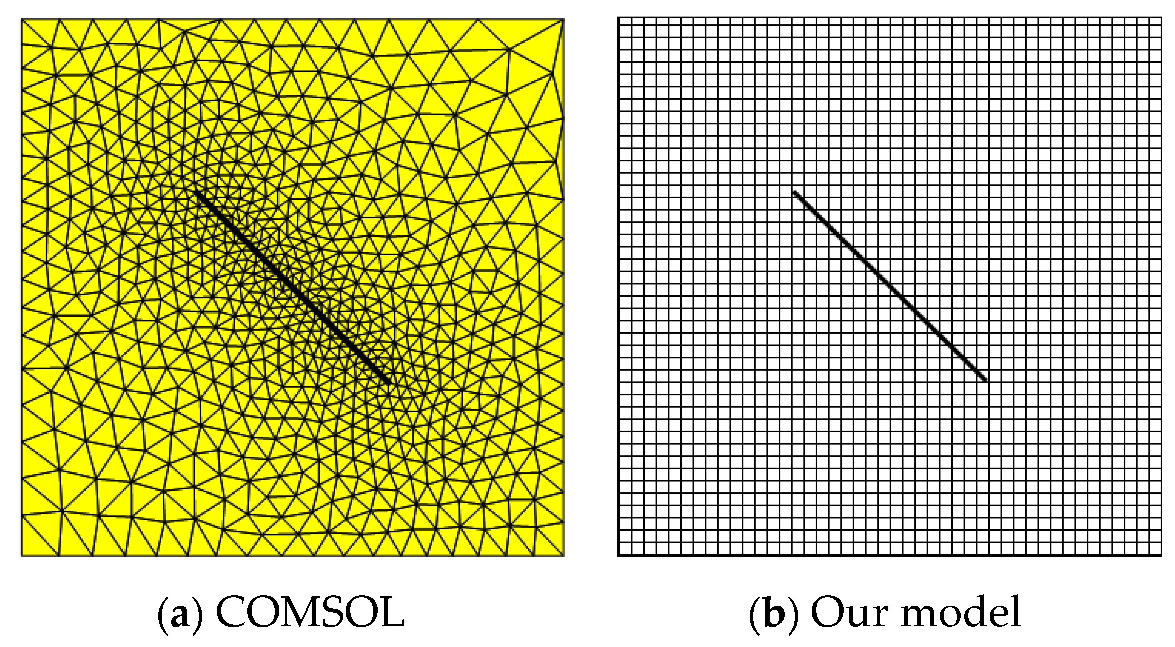
3. Numerical Discretization

Equations (7), (29), and (30) are the equations to be solved, and the finite volume method was used to discretize these three equations in space and time [45]. The solution of discrete equations in time has implicit first-order accuracy, whereas discrete equations in space combine implicit and explicit methods with second-order accuracy. OpenFOAM 5.0 was used as the solver for fully coupled models. Stress balance Equation (7) can be expressed as

$$\begin{array}{c}{\displaystyle {\oint }_{\partial V}ds\cdot \left[\left(2\mu +\lambda \right)\nabla u\right]}=-{\displaystyle {\int }_{\partial V}ds\cdot \left[\mu \nabla u^T+\lambda Itr\left(\nabla u\right)-\left(\mu +\lambda \right)\nabla u\right]}\\ +{\displaystyle {\oint }_{\partial V}ds\cdot \left(bpI\right)-{\displaystyle {\oint }_{\partial V}ds\cdot \left(b{p}_{0}I+{\sigma }_0\right)}}\end{array}$$

(31)

The left term of Equation (31) is an implicit surface diffusion term, and the right term is an explicit surface diffusion term followed by an explicit pressure coupling term and an explicit constant term representing the initial state. Based on the finite volume method, discretizing the flows in Equation (29) into a matrix can result in the following:

$$\begin{array}{l}{\displaystyle {\int }_V\left[\left({\varphi }_{\mathrm{m}}{c}_{\mathrm{g}}+\frac{b-\varphi }{K_{\mathrm{s}}}\frac{m_{\mathrm{ad}}}{{\rho }_{\mathrm{g}}}+\frac{b^2}{K_{\mathrm{dr}}}\right)\frac{\partial p^n}{\partial t}\right]dV-{\displaystyle {\oint }_{\partial V}ds\cdot \left(\frac{{\displaystyle \prod _i{F}_{\mathrm{app},i}}k}{{\mu }_{\mathrm{g}}}\nabla p^n\right)}}=\\ {\displaystyle {\int }_V\left(\frac{b^2}{K_{\mathrm{dr}}}\frac{\partial p^{n-1}}{\partial t}\right)}dV-{\displaystyle {\oint }_{\partial V}ds\cdot \frac{\partial u}{\partial t}-{\displaystyle {\int }_V\left[{\lambda }_t{T}_{\mathrm{f}-\mathrm{m}}\left(p_{\mathrm{f}}^n-p^n\right)\right]dV}}\end{array}$$

(32)

The first term on the left of the equal sign in the equation represents the pressure term of the current time step, and the second term represents the implicit pressure flow term of the current time step. The discretization method of the fluid flow equation for fractures (Equation (30)) is similar to Equation (32).

$$\begin{array}{l}{\displaystyle {\int }_V\left[\left(\frac{1}{M_{\mathrm{f}}}+\frac{b^2}{K_{\mathrm{dr}}}\right)\frac{\partial p_n^f}{\partial t}\right]dV-{\displaystyle {\oint }_{\partial V}ds\cdot \left(\frac{{\displaystyle \prod _i{F}_{\mathrm{app},i}}{k}_f}{{\mu }_{\mathrm{g}}}\nabla p_f^n\right)}}={\displaystyle {\int }_V\left(\frac{b^2}{K_{\mathrm{dr}}}\frac{\partial p_{\mathrm{f}}^{n-1}}{\partial t}\right)}dV\\ -{\displaystyle {\oint }_{\partial V}ds\cdot \frac{\partial u}{\partial t}-{\displaystyle {\int }_V\left[{\lambda }_{\mathrm{t}}{T}_{\mathrm{f}-\mathrm{m}}\left(p^n-p_{\mathrm{f}}^n\right)\right]dV-}}{\displaystyle {\int }_V\left[{\lambda }_{\mathrm{t}}{T}_{\mathrm{f}-\mathrm{f}}\left(p_{\mathrm{f}1}^n-p_{\mathrm{f}2}^n\right)\right]dV}+{\displaystyle {\int }_{V}qdV}\end{array}$$

(33)

After discretization of the above three equations, the matrix with five unknowns (u_x, u_y, u_z, p, p_f) can be solved successively using the Newton–Raphson iterative method. It is a matrix composed of three displacement equations, coefficient matrices of the fluid flow equations in the matrix, and cracks. After obtaining the displacement component and pressure, the effective and total stresses were calculated.

$$\left(\begin{array}{l}{A}_{\mathrm{mm}} A_{\mathrm{mf}}\\ A_{\mathrm{fm}} A_{\mathrm{ff}}\end{array}\right)\left(\begin{array}{l}{P}_{\mathrm{m}}\\ P_{\mathrm{f}}\end{array}\right)=\left(\begin{array}{l}{B}_{\mathrm{m}}\\ B_{\mathrm{f}}\end{array}\right)$$

(34)

$$\left[X\right]\left[U\right]=\left[R\right]$$

(35)

where $A_{\mathrm{mm}}$ and $A_{\mathrm{ff}}$ are diagonal sub-matrix blocks, representing the conductivity in the matrix grid and the conductivity in the fracture grid, respectively; $A_{\mathrm{mf}}$ and $A_{\mathrm{fm}}$ are off-diagonal sub-matrix blocks, representing the conductivity between the matrix and the fracture; $P_{\mathrm{m}}$ and $P_{\mathrm{f}}$ represent the pressure sub-matrix in matrix and fracture, respectively; $X$ represents the coefficient matrix. $U$ are displacement matrix; $R$ is known constant items. Equations (34) and (35) are solved sequentially by iterative method, respectively. This article mainly uses the sequential coupling iterative method to solve the displacement equation and fluid flow equation in the model. When the two coefficient matrices reach convergence, they enter the next step of calculation. After the displacement component is obtained, the effective stress and total stress can be further calculated using the stress–strain relationship.

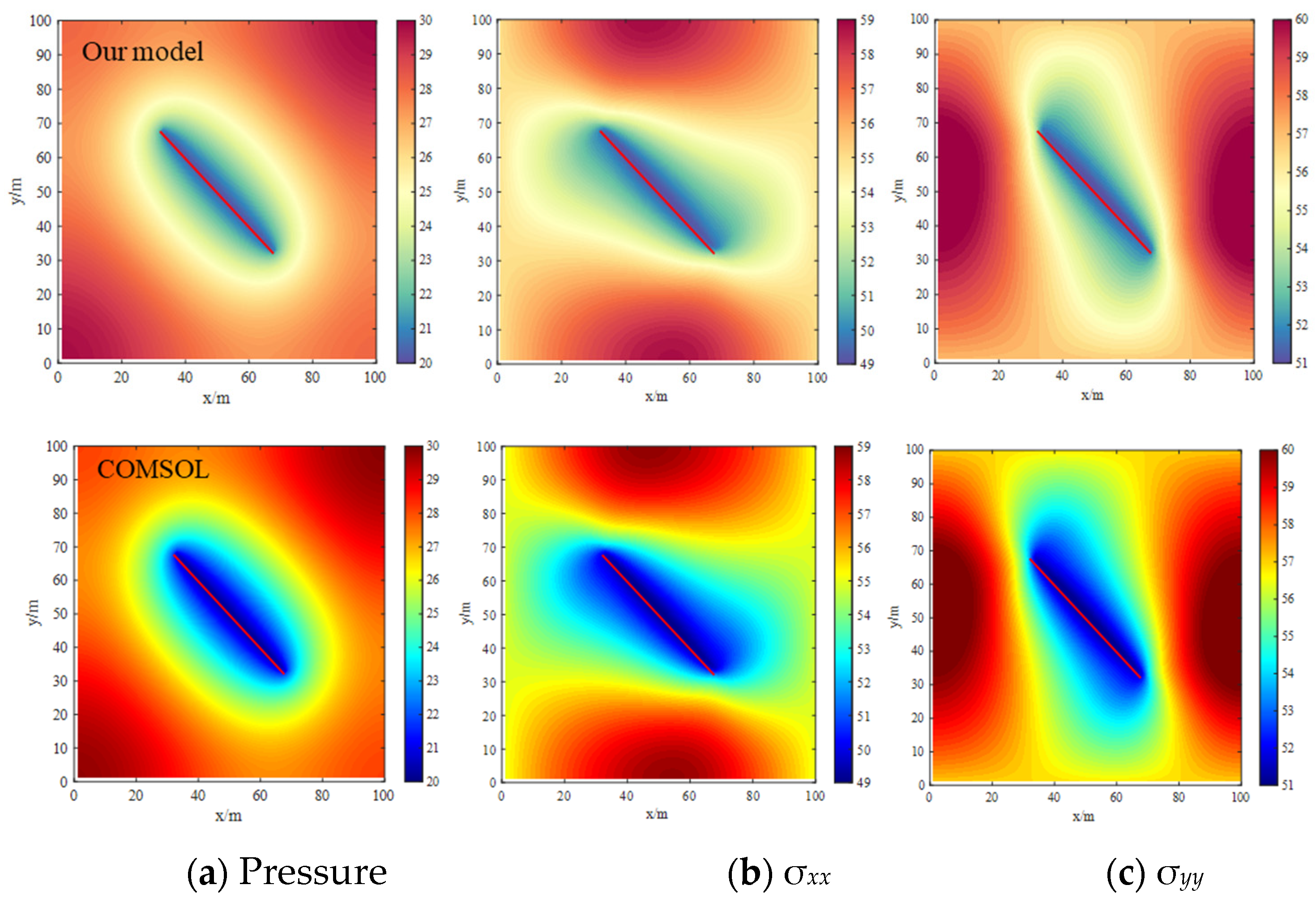
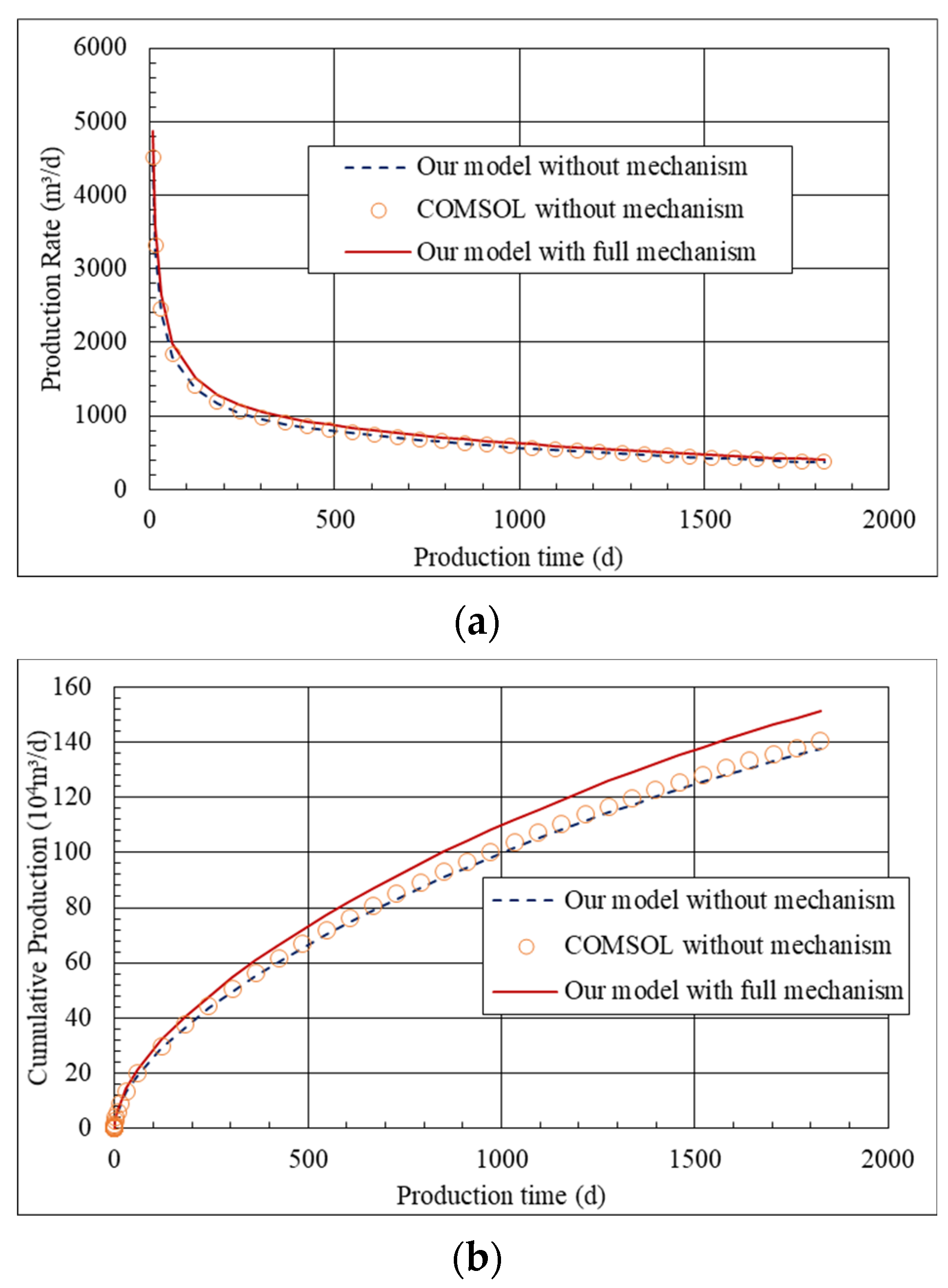
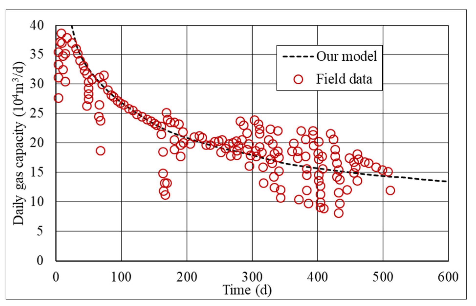
4. Model Verification

To verify the accuracy of our model in stress and productivity calculations, two single-fracture production-induced stress models with an approaching angle of 45° were established using our model and COMSOL commercial software, using structured and unstructured grids, respectively. The grid division of the two physical models is shown in Figure 2. The dimensions of the domain are 100 m (x) × 100 m (y) × 20 m (z). The number of structured grids in Figure 2a is 2500, and the number of unstructured grids is 1468 (Figure 2b). The constrained displacement boundary condition is used; that is, the displacement on the boundary is set to be 0 in the direction perpendicular to the boundary of the model. The constrained displacement boundary condition is adopted in the simulation. Zero normal displacement boundary conditions, i.e., roller boundaries, are applied to the lateral and bottom boundaries, and there is no fluid flow. The input parameters are shown in

Table 1. The main input parameters in model validation.

Parameters	Unit	Value	Parameters	Unit	Value
Initial pressure	MPa	40	Fracture half-length	m	100
Langmuir pressure	MPa	4	Reservoir permeability	nD	300
formation temperature	K	343.15	Fracture permeability	D	2
Langmuir volume	m3/kg	0.018	Fracture width	m	1 × 10−3
Matrix porosity	-	0.06	Bottom hole pressure	MPa	20
Matrix compressibility coefficient	1/MPa	1.0 × 10−3	Time	years	5
Fracture porosity	-	1.0	The dimensions of the domain (x, y, z)	m	(100, 100, 20)
Young’s modulus	GPa	26	Stress along the x-axis	MPa	55
Poisson’s ratio	-	0.15	Stress along the y-axis	MPa	57
Biot coefficient	-	0.8	Stress along the z-axis	MPa	58

, and the distribution cloud diagram of pore pressure, σ_xx stress along the x-axis, and σ_yy stress along the y-axis direction is obtained through simulation, as shown in Figure 3. Figure 4 shows the production rate and cumulative production based on our model and COMSOL software. Comparing Figure 3a and Figure 3b, the results calculated by our model are very close to the results calculated by COMSOL software. The results in Figure 4 also show that the production rate and cumulative production obtained by our model without considering any mechanism are basically consistent with the results of COMSOL. The data in Figure 4 that are significantly larger than the simulation results based on COMSOL are the results obtained by our model considering the effects of adsorption and desorption, diffusion, and slippage mechanisms. Overall, our model has high accuracy for both stress and production simulations.

In addition, field data are also used to validate our model. Taking a Fuling shale gas well as an example, the basic parameters of the well are as follows: The thickness of the shale reservoir is 38 m, the length is 2500 m, the width is 600 m, and the shaft length is 1600 m. The original formation pressure is 36.49 MPa, the bottom hole pressure is 20.9 MPa, the formation temperature is 82.2 °C, the formation permeability is 3.5 × 10⁻⁵ mD, and the matrix porosity is 5.46%. The Langmuir volume is 3 × 10⁻³ m³/kg, the Langmuir pressure is 5 MPa, the hydraulic fracture conductivity is 0.5 D·cm, the fracture half-length is 120 m, the permeability in the reformed area is 0.05 mD, and the number of fracturing stages is 15. The gas viscosity is 0.022 mPa·s, and the matrix compression coefficient is 4.4 × 10⁻⁴ MPa⁻¹. Based on the above parameters and the model proposed in this paper, the corresponding numerical model is established. The simulation results are shown in Figure 5. It can be seen from the calculation results that the simulation results are basically consistent with the field production data, which proves the accuracy of our model.

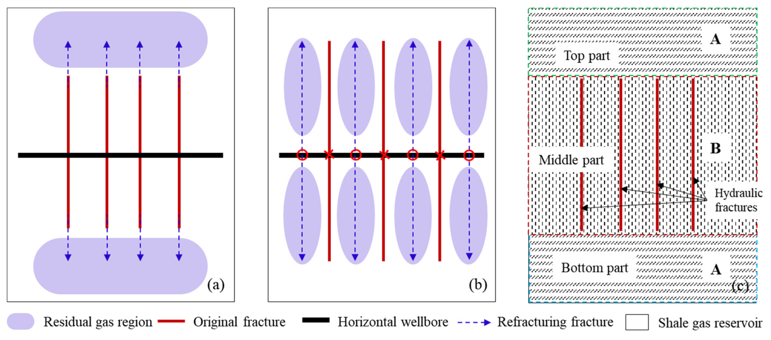
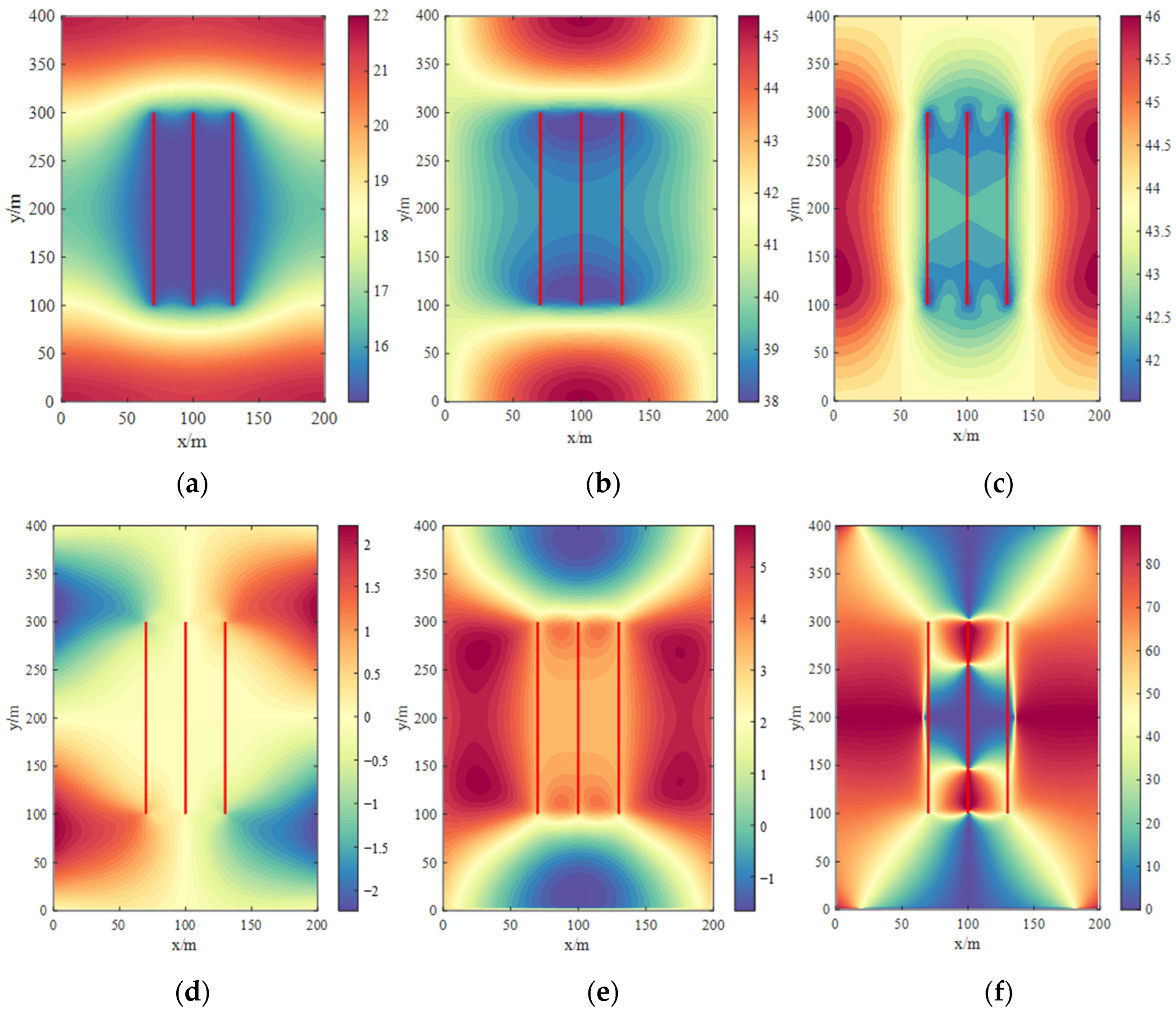
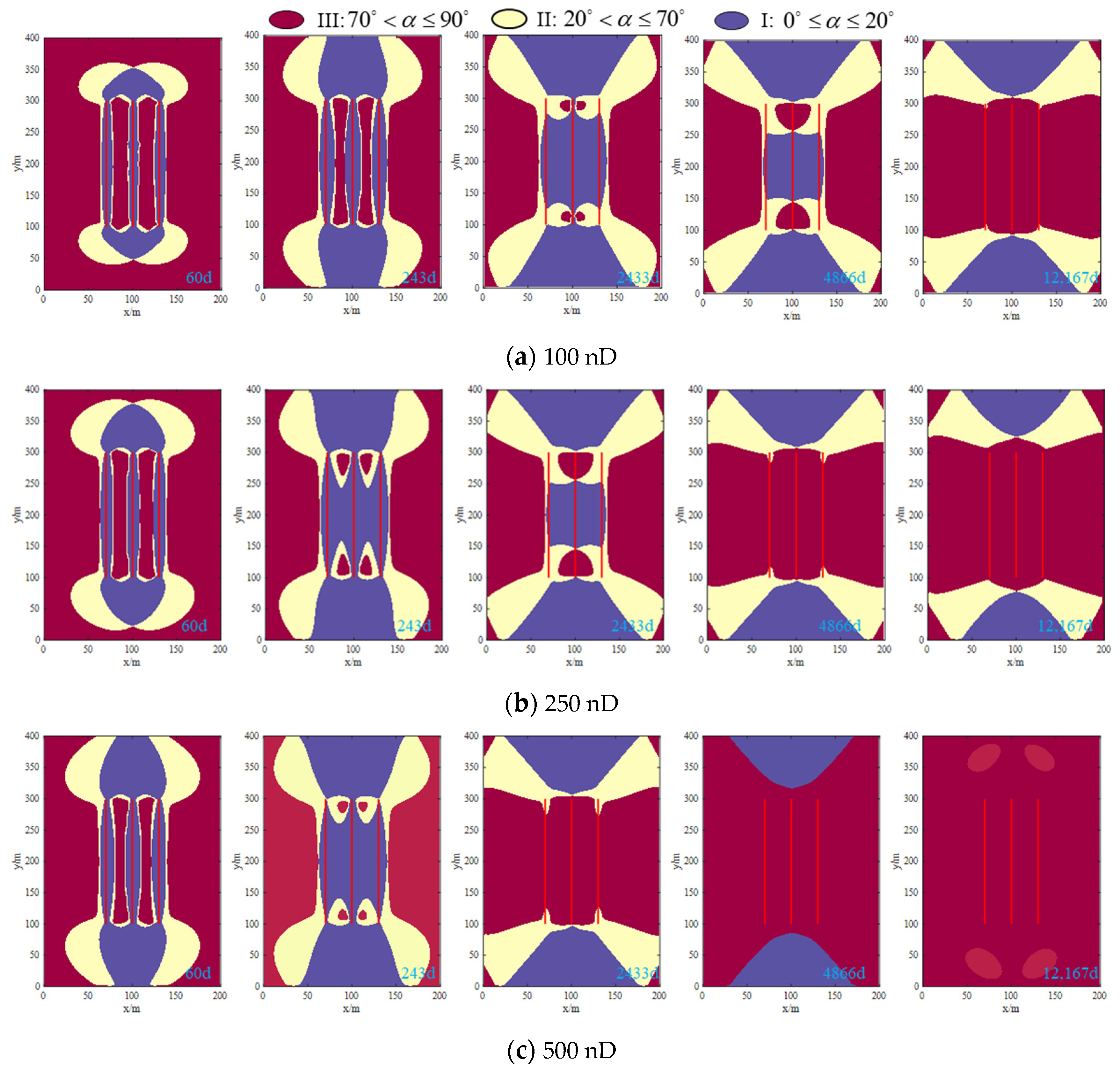
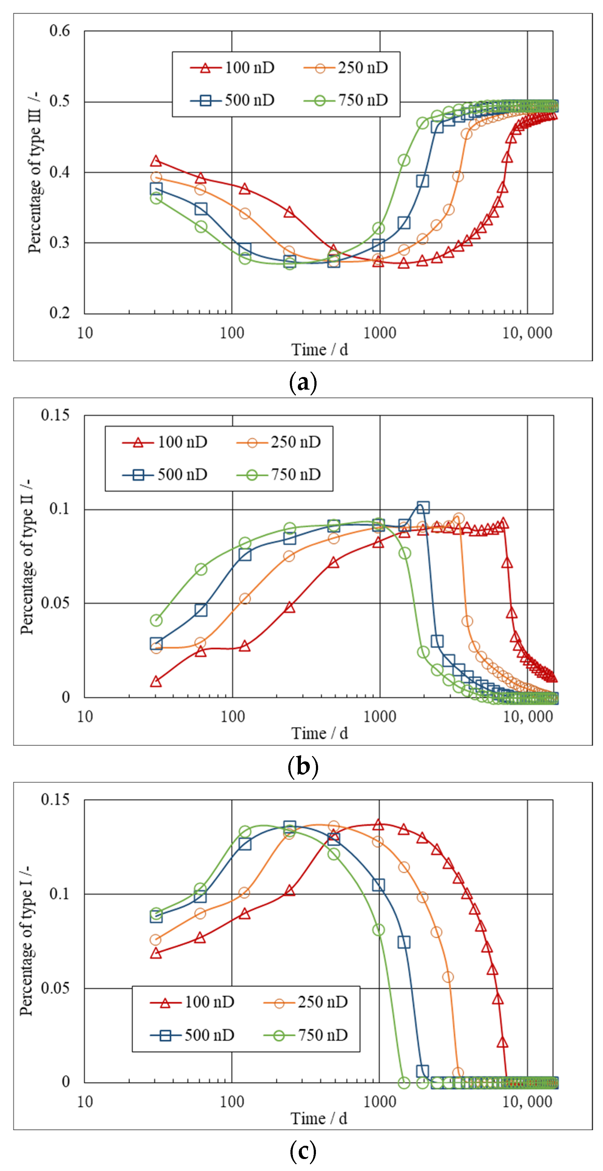
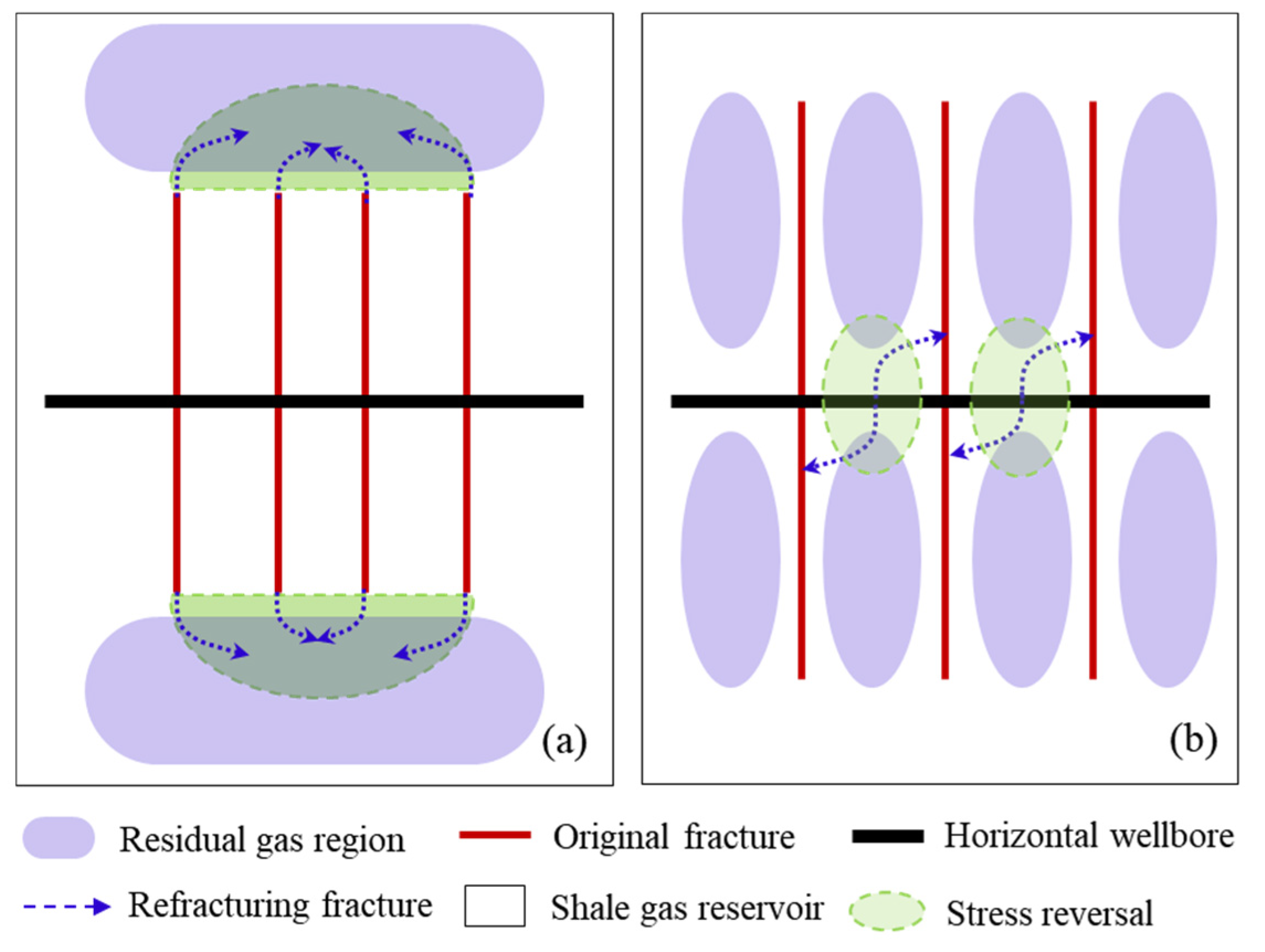
5. Evolution Law of Stress Field and Timing Analysis of Refracturing

One of the keys to refracturing design is the choice of refracturing timing. According to the basic understanding that the extension direction of tensional hydraulic fractures is perpendicular to the orientation of the minimum horizontal stress (that is, along the orientation of the maximum horizontal stress), it is known that the key factors affecting the timing of refracturing are the magnitude and direction of the maximum horizontal stress and the minimum horizontal stress before refracturing. In this section, the effects of permeability, initial stress difference, cluster spacing, and fracture half-length on the reorientation of the maximum horizontal stress are simulated. Based on the potential excavation area corresponding to the two types of refracturing methods, the percentages of different stress orientation ranges in Parts A and B were calculated, and the corresponding refracturing timings were determined.

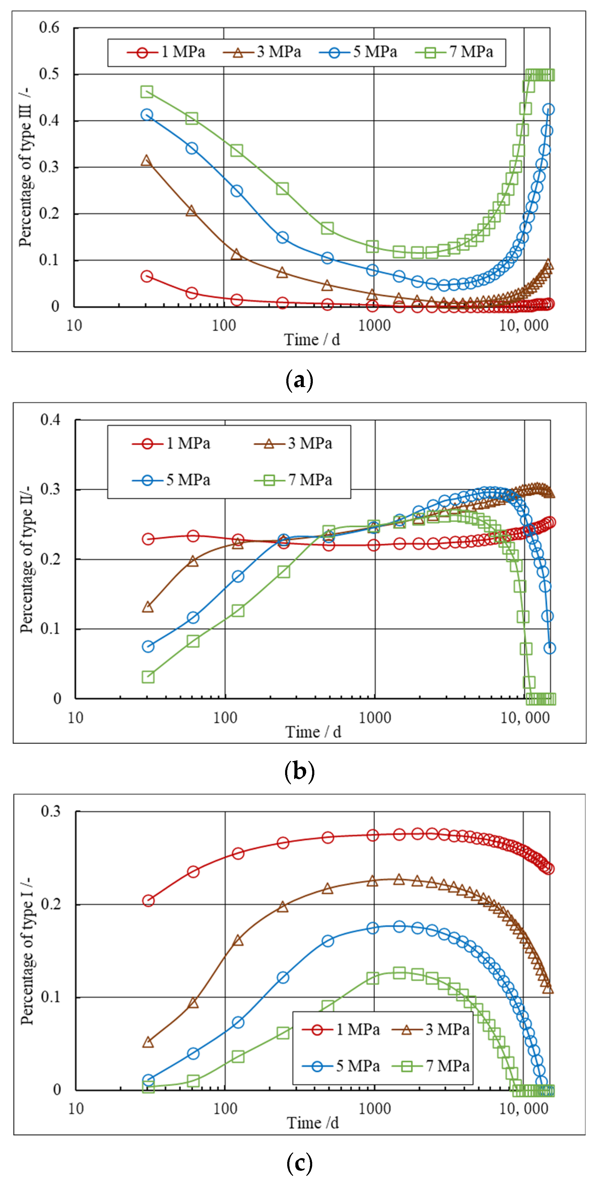
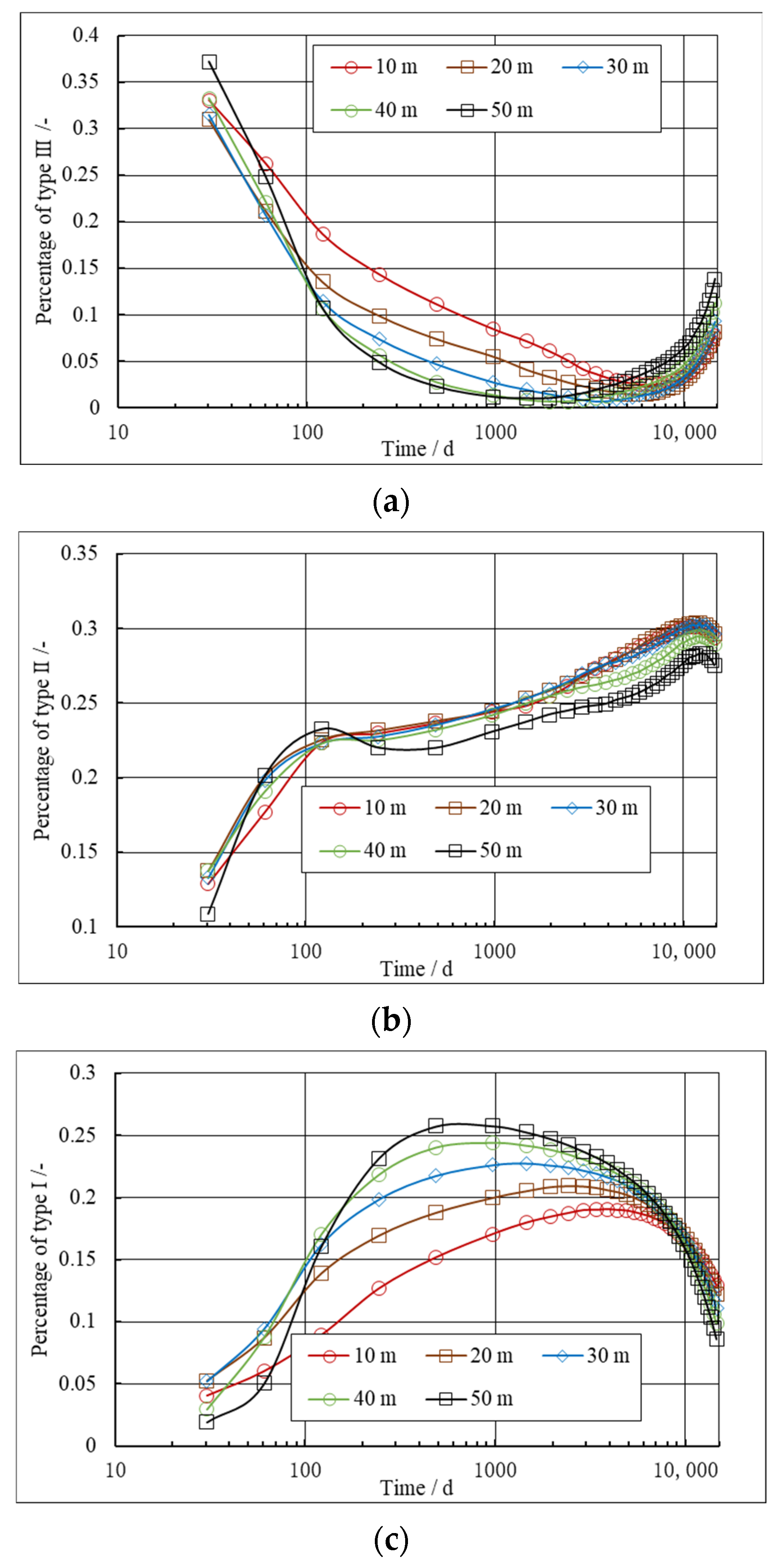
5.1. Effect of Permeability on Stress Orientation and Refracturing Timing

The generation of a pore pressure gradient is the fundamental cause of the stress field variation. Permeability determines the fluid flow efficiency and has an important effect on the pressure distribution during shale gas drainage. To study the influence of permeability on the stress field and refracturing timing, a single-stage shale gas drainage model with three clusters of hydraulic fractures, 100 m fracture half-length, and 30 m cluster spacing was established according to the proposed model and the parameters listed in

Table 2. Main input parameters.

Parameters	Unit	Value	Parameters	Unit	Value
Matrix compression coefficient	1/MPa	4.4 × 10−4	Initial stress along y-axis	MPa	44
Matrix permeability	nD	100–750	Initial stress along z-axis	MPa	45
Elastic modulus	GPa	24	Time	years	40
Poisson ratio	-	0.15	The dimensions of the domain (x, y, z)	m	(200, 400, 20)
Initial stress along x-axis	MPa	41	Biot coefficient	-	0.8

. All parameters, in this case, are mainly obtained from on-site logging data and construction data. The distribution of the reservoir pressure, ${\sigma }_{xx}$ stress along the x-axis direction, ${\sigma }_{\mathrm{yy}}$ stress along the y-axis direction, ${\sigma }_{\mathrm{xy}}$ shear-induced stress, $\Delta \sigma$ horizontal stress difference, and orientation of the maximum horizontal stress after 2433 d of production were obtained through simulation, as shown in Figure 6. As shown in Figure 6a–e, the stress distribution in the reservoir shows strong heterogeneity owing to the depletion of pressure. ${\sigma }_{xx}$ and ${\sigma }_{yy}$ decreased significantly near the fracture, whereas they increased significantly in the region around the fracture to support the depletion of pressure, resulting in negative horizontal stress differences in the top and bottom parts of the domain (Figure 6e). To explore the means to optimize the timing of the two types of refracturing, the orientation of the maximum horizontal principal stress is mainly considered as the analysis object in this section. The orientation of the maximum horizontal principal stress is calculated as follows:

$$\left.\begin{array}{l}{\sigma }_{\mathrm{H}}\\ {\sigma }_{\mathrm{h}}\end{array}\right\}={\displaystyle \frac{{\sigma }_{xx}+{\sigma }_{yy}}{2}}\pm \sqrt{{\left({\displaystyle \frac{{\sigma }_{xx}-{\sigma }_{yy}}{2}}\right)}^2+{\sigma }_{xy}^2}$$

(36)

$$\tan \left(\alpha \right)={\displaystyle \frac{{\sigma }_{\mathrm{H}}-{\sigma }_{xx}}{{\sigma }_{xy}}}$$

(37)

where $\alpha$ is the angle between the maximum horizontal stress and the x-axis, which represents the orientation of the maximum horizontal stress. The initial $\alpha$ is 90°. ${\sigma }_{xx}$ and ${\sigma }_{\mathrm{yy}}$ are the stresses along the x- and y-axes, respectively. ${\sigma }_{x\mathrm{y}}$ represents the induced shear stress. ${\sigma }_{\mathrm{H}}$ and ${\sigma }_{\mathrm{h}}$ represent the maximum and minimum horizontal stresses, respectively. According to Equation (37) and the results shown in Figure 6b–d, the distribution of the orientation of ${\sigma }_{\mathrm{H}}$ in the domain can be calculated (Figure 6f). To facilitate analysis of the fracture propagation trajectories during refracturing, the orientation of the maximum horizontal stress was divided into Types I, II, and III. Type I indicates that stress inversion has occurred, $0^{\circ }\le \alpha \le {20}^{\circ }$; Type II indicates that the turning degree is strong, ${20}^{\circ }<\alpha \le {70}^{\circ }$; and Type III indicates less stress reorientation, ${70}^{\circ }<\alpha \le {90}^{\circ }$. As shown in Figure 6a, three types of reorientation regions are distinguished by three colors to determine the fracture propagation trajectory according to different colors. Considering that the target areas of “extending the original fractures (Method I)” and “plugging the old fractures and refracturing the new fractures (Method II)” of the two refracturing methods belong to Part A and Part B, respectively, as shown in Figure 1.

Figure 7 shows the distribution of the maximum horizontal stress orientation under different matrix permeabilities and times. Figure 8 and Figure 9 show the relationship between the percentages of the three types of reorientation areas in Region A and Region B with time and matrix permeability, respectively. According to Figure 1c, the total area of the simulation domain S = S_A + S_B, and the percentage of the three types of reorientation area in the region can be expressed as

$${\eta }_{\mathrm{I}}={\displaystyle \frac{S_{\mathrm{I}}}{S}} ; {\eta }_{\mathrm{II}}={\displaystyle \frac{S_{\mathrm{II}}}{S}}; {\eta }_{\mathrm{III}}={\displaystyle \frac{S_{\mathrm{III}}}{S}} \mathrm{\Omega }\mathrm{A} \mathrm{or} \mathrm{B}$$

(38)

where $S_{\mathrm{I}}$ is the area of I ($0^{\circ }\le \alpha \le {20}^{\circ }$), $S_{\mathrm{II}}$ is the area of II (${20}^{\circ }<\alpha \le {70}^{\circ }$), $S_{\mathrm{III}}$ is the area of III ($\alpha >{70}^{\circ }$), and ${\eta }_{\mathrm{I}}$, ${\eta }_{\mathrm{II}}$, and ${\eta }_{\mathrm{III}}$ represent the ratios of Types I, II, and III in Regions A or B to the total area, respectively. By comparing Figure 7, Figure 8 and Figure 9, the percentage of Type III areas in the domain first decreased and then increased with time, whereas the percentage of Type II and Type I areas first increased and then decreased with time. With an increase in permeability, the shortest time was used for the percentage of the three types of areas to reach the maximum value. That is, the higher the permeability, the faster the maximum horizontal stress orientation returns to its initial state. For the two refracturing methods shown in Figure 1, the original expectation is that the fractures could extend along the y-axis and pass through the potential remaining oil and gas distribution area. However, Figure 7 shows that after a period of production, Type I stress inversion zones appeared near the perforations and at the ends of the fractures. If these two refracturing measures are implemented at this time, the new fracture may deviate from the target area or intersect with the existing fracture (Figure 10), such that the refracturing cannot achieve the desired effect. Therefore, the key to choosing the timing of refracturing is to avoid the period when the area percentage of Type I is large and make the fractures expand along the y-axis direction as much as possible. According to this principle, combined with Figure 8c, when the matrix permeability was 750 nD, the area percentage of Type I in Region A after 7000 d of production was 0. At this time, if Method I is implemented, the fracture will be along the y-axis extending through the target potential tapping area; therefore, 7000 d is the optimal timing for this refracturing method, and Figure 9c shows that if Method II is used when the matrix permeability is 750–100 nD, the timing of refracturing should be approximately 2000–6800 d. Comparing Figure 8c and Figure 9c, it can be observed that as the permeability decreases, the longer the time required for the stress orientation to recover, the longer the time corresponding to the timing of refracturing. In addition, the actual refracturing timing optimization must consider whether the target area is sufficiently valuable to produce.

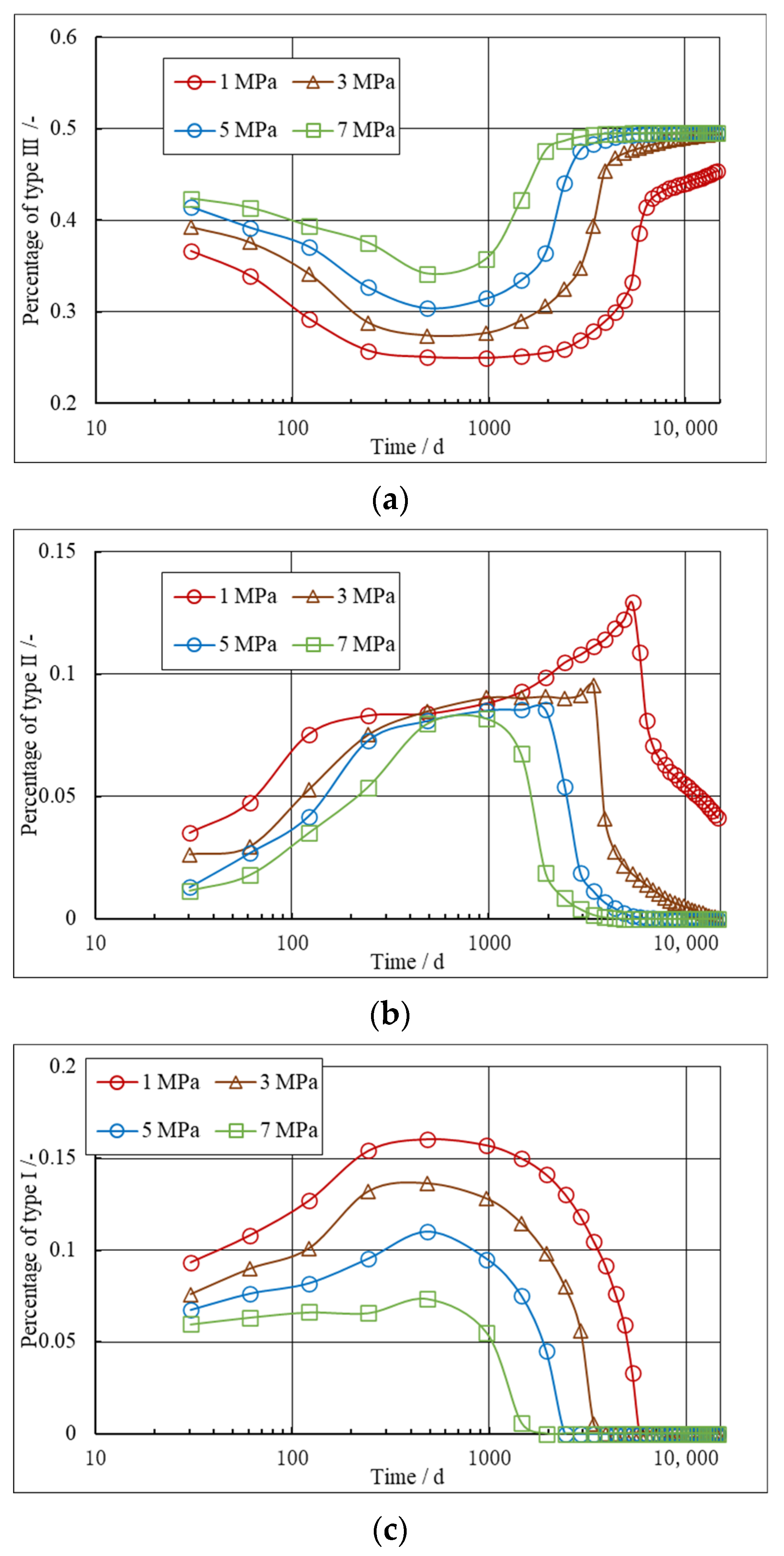
5.2. Effect of Initial Stress Difference on Stress Orientation and Refracturing Timing

Based on the model and parameters described in Section 5.1, the initial stress differences were set to 1, 3, 5, and 7 MPa, respectively, and the distributions of the three types of reorientation areas at different times were simulated, as shown in Figure 11. Figure 12 and Figure 13 show the relationship between the three types of reorientation percentages, time, and initial stress difference in Regions A and B, respectively. Comparing Figure 11, Figure 12 and Figure 13, when the stress difference is small, the percentage of Type III in Region A does not show an evident trend of first decreasing and then increasing, whereas the percentage of Type II does not show a trend of first increasing and then decreasing. The analysis of Figure 12 and Figure 13 shows that the larger the initial stress difference, the larger the area of Type III and the smaller the area of Type I simultaneously, and the easier it is for the maximum horizontal stress to return to the initial state. Figure 12c shows that the greater the initial stress difference, the earlier the time to adopt refracturing Method I. For example, when the initial stress difference was 7 MPa, the time for the Type I reorientation area to disappear was approximately 8950 d. From the analysis of Figure 13c, when the initial stress difference was 1–7 MPa, the time taken to adopt refracturing Method II was 5500–1460 d. Compared with refracturing Method I, the timing of refracturing Method II is earlier. For reservoirs with a large initial stress difference, such as that exceeding 10 MPa, the timing of refracturing has an earlier window period.

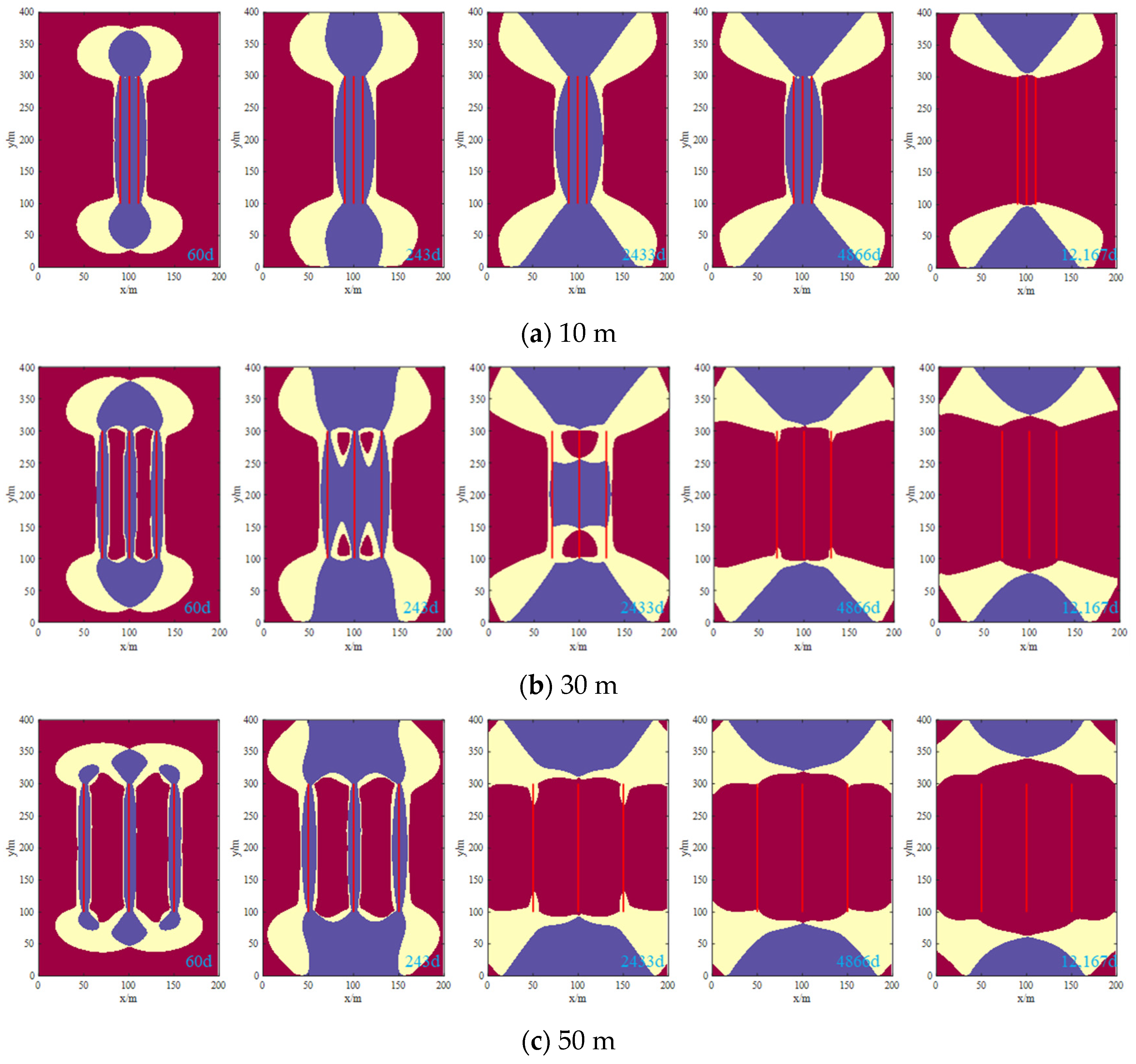
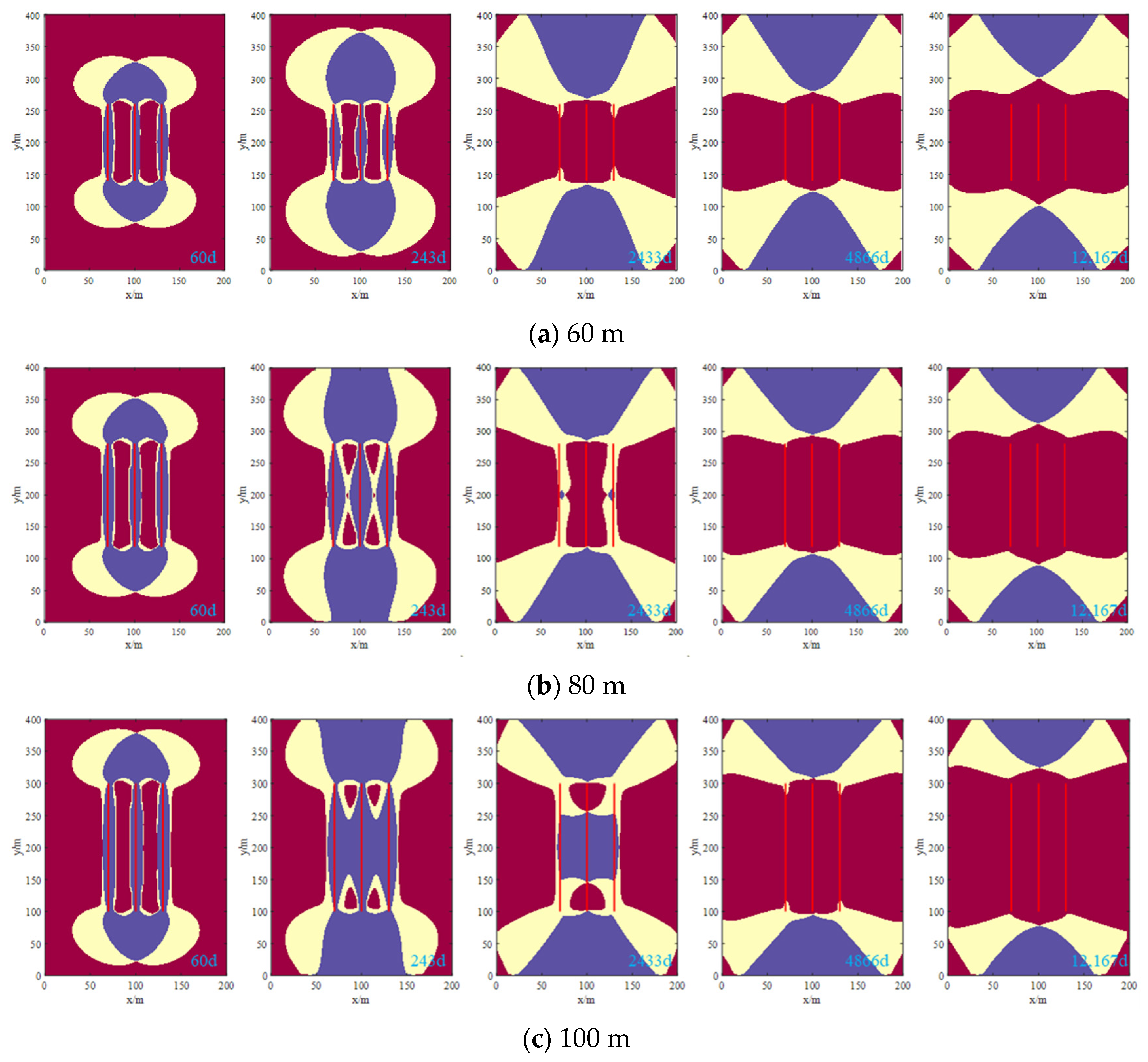
5.3. Influence of Cluster Spacing on Stress Orientation and Refracturing Timing

In the early development of oilfields, the cluster spacing of the staged multi-cluster fracturing design was relatively large, and the transmission capacity of the high-permeability fracture channels was limited, which constrained the increase in production. Therefore, it is of great significance to study the effect of cluster spacing on the timing of refracturing. In addition, according to the model and parameters in Section 5.1, the fracture cluster spacing was changed from 10 m to 50 m, and the distribution of the three types of stress reorientation areas at different times was simulated, as shown in Figure 14. Figure 15 and Figure 16 show the relationship among the three types of reorientation area percentages, logarithmic production time, and cluster spacing in Area A and Area B, respectively. Figure 14 shows that the larger the cluster spacing, the easier it is for the maximum horizontal stress orientation in Region B to return to its initial state. It can be observed from Figure 15c that, under the conditions of this case, the timing of using refracturing Method I exceeded 15,000 d; as the cluster spacing increased, the timing of refracturing Method I was slightly earlier. By analyzing Figure 16c, it can be found that the cluster spacing has a greater effect on refracturing Method II. As the cluster spacing increases, the timing of refracturing Method II becomes earlier. Under these conditions, the cluster spacing was 60–120 m, and the corresponding time for refracturing Method II was 10,000–140 d.

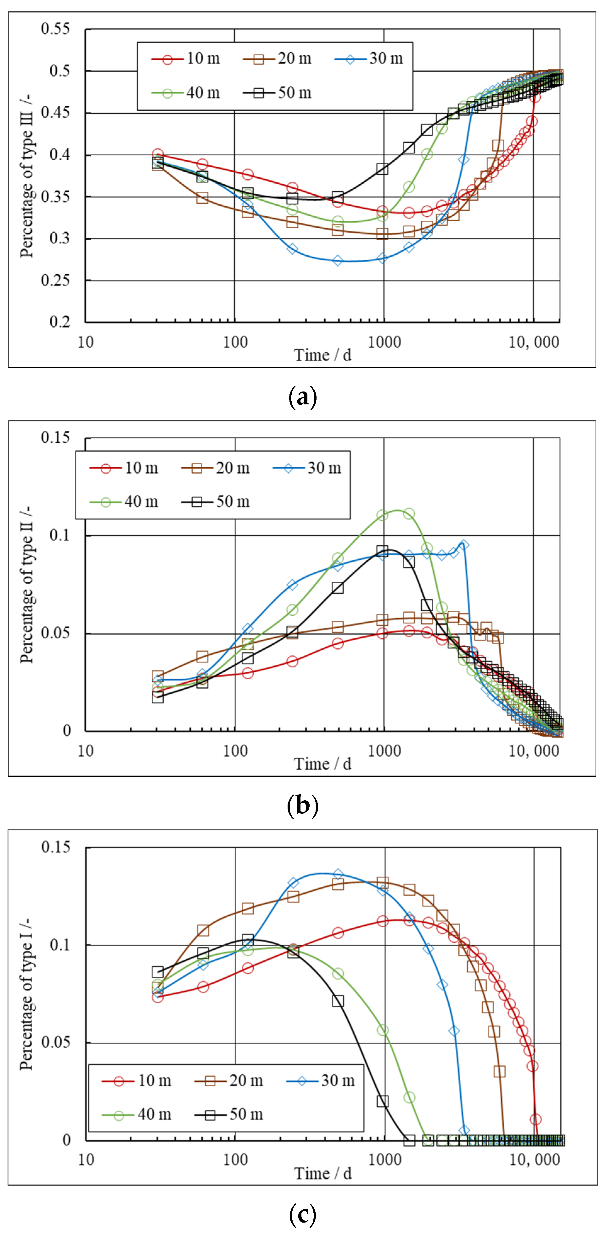
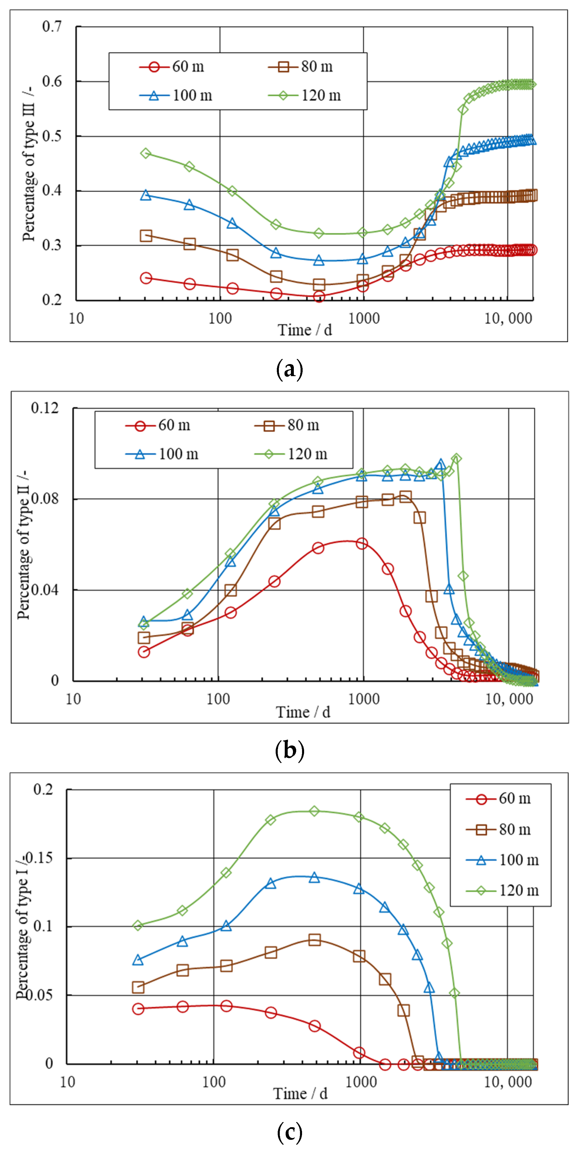
5.4. Influence of Fracture Half-Length on Stress Orientation and Refracturing Timing

The length of the fracture represents different scales of fracturing operations and can also reflect situations in which the fracture length of certain fracturing stages is relatively short because of the suspension of fracturing construction for special reasons. It is also meaningful to study the influence of the fracture half-length on the changing law of refracturing timing. According to the model and parameters in Section 5.1, the distribution of the three types of stress reorientation areas under different fracture half-lengths was simulated under a cluster spacing of 30 m, an initial stress difference of 3 MPa, and a matrix permeability of 250 nD, as shown in Figure 17. Figure 18 and Figure 19 show the relationship among the three types of reorientation area percentages, logarithmic production time, and fracture half-length in Regions A and B, respectively. An analysis of Figure 18c shows that with an increase in the fracture’s half-length, the smaller the percentage of the Type I area, the earlier the time to adopt refracturing Method I, but it exceeded 16,000 d in all cases. However, Figure 19c shows that with an increase in the fracture half-length, the timing of adopting refracturing Method II was adopted later. Under the conditions in this case, the range of the fracture half-length was 60–120 m, and the corresponding time for refracturing Method II was 1000–4380 d.

6. Conclusions

Based on the EDFM and FVM, a model of stress evolution coupled with fluid flow/geomechanics was successfully developed, considering the adsorption, desorption, diffusion, and slippage flow of shale gas. The model achieves the coupled simulation of complex natural fractures, hydraulic fractures, storage and transport mechanisms, and stress- and pore-elastic effects and can more accurately predict the stress distribution. The accuracies of the stress and production calculations for the proposed model were verified using a COMSOL commercial simulator. The following conclusions were drawn from the simulations:

1. The principle of selecting the timing of refracturing methods I and II is to avoid the time window where the percentage of Type I stress reorientation area is relatively large so that the fractures can expand along the y-axis direction (vertical to horizontal well) as much as possible;

2. With the decrease in permeability, the time required for the recovery of the maximum horizontal stress orientation is longer, and the timing of refracturing is also later. When the permeability range is 750–100 nD, the time window of refracturing Method I is 7000 d < t_o, and the time window of refracturing Method II is 2000 d < t_o < 6800 d;

3. The larger the initial stress difference, the larger the reorientation area of Type III and the smaller the reorientation area of Type I simultaneously, and the easier the orientation of the maximum horizontal stress to return to the initial state. The greater the initial stress difference, the earlier the timing of refracturing Method I. When the initial stress difference range was 7–1 MPa, the time window of refracturing Method I was 8950 d < t_o, and that of refracturing Method II was 1460 d < t_o < 5500 d;

4. With an increase in cluster spacing, the timing of refracturing becomes earlier. When the cluster spacing range was 50–10 m, the time window of refracturing Method I was 15,000 d < t_o, and that of refracturing Method II was 1460 d < t_o < 10,000 d;

5. With the increase in fracture half-length, the timing of refracturing Method I is earlier, and the timing of refracturing Method II is later. When the fracture half-length is 120 –60 m, the time window of refracturing Method I is 16,000 d < t_o, and the time window of refracturing Method II is 4380 d > t_o > 1000 d.

A new refracturing time optimization method was proposed for the two types of refracturing methods. This method and the inferences from it are of great significance for the theory and design of refracturing.

References

1. Chen, H.; Ji, B.; Wei, B.; Meng, Z.; Li, Y.; Lu, J.; Tang, J. Experimental simulation of enhanced oil recovery on shale rocks using gas injection from material to characterization: Challenges and solutions. Fuel 2024, 356, 129588. [Google Scholar] [CrossRef]
2. Chen, H.; Li, H.; Li, Z.; Li, S.; Wang, Y.; Wang, J.; Li, B. Effects of matrix permeability and fracture on production characteristics and residual oil distribution during flue gas flooding in low permeability/tight reservoirs. J. Pet. Sci. Eng. 2020, 195, 107813. [Google Scholar] [CrossRef]
3. Guo, X.; Wu, K.; An, C.; Tang, J.; Killough, J. Numerical Investigation of Effects of Subsequent Parent-Well Injection on Interwell Fracturing Interference Using Reservoir-Geomechanics-Fracturing Modeling. SPE J. 2019, 24, 1884–1902. [Google Scholar] [CrossRef]
4. Heidari, S.; Li, B.; Jacquey, A.B. Finite element modeling of wellbore stability in a fractured formation for the geothermal development in northern Quebec, Canada. Geoenergy Sci. Eng. 2023, 231, 212350. [Google Scholar] [CrossRef]
5. Liu, L.J.; Liu, Y.; Yao, J.; Huang, C. Efficient coupled multiphase-flow and geomechanics modeling of well performance and stress evolution in shale-gas reservoirs considering dynamic fracture properties. SPE J. 2019, 25, 1523–1542. [Google Scholar] [CrossRef]
6. Safari, R.; Lewis, R.; Ma, X.; Mutlu, U.; Ghassemi, A. Fracture curving between tightly spaced horizontal wells. In Proceedings of the Unconventional Resources Technology Conference, San Antonio, TX, USA, 20–22 July 2015. [Google Scholar]
7. Safari, R.; Lewis, R.; Ma, X.; Mutlu, U.; Ghassemi, A. Infill-well fracturing optimization in tightly spaced horizontal wells. SPE J. 2017, 22, 582–595, SPE-178513-PA. [Google Scholar] [CrossRef]
8. Pei, Y.; Sepehrnoori, K. Investigation of Parent—Well Production Induced Stress Interference in Multilayer Unconventional Reservoirs. Rock Mech. Rock Eng. 2022, 55, 2965–2986. [Google Scholar] [CrossRef]
9. Wang, Q.; Hu, Y.; Zhao, J.; Chen, S.; Fu, C.; Zhao, C. Numerical simulation of fracture initiation, propagation and fracture complexity in the presence of multiple perforations. J. Nat. Gas Sci. Eng. 2020, 83, 103486. [Google Scholar] [CrossRef]
10. Kumar, D.; Ghassemi, A. 3D geomechanical analysis of refracturing of horizontal wells. In Proceedings of the Unconventional Resources Technology Conference, Austin, TX, USA, 24–26 July 2017. [Google Scholar] [CrossRef]
11. Wang, J.; Olson, J.E. Auto-optimization of hydraulic fracturing design with three-dimensional fracture propagation in naturally fractured multi-layer formations. In Proceedings of the SPE/AAPG/SEG Unconventional Resources Technology Conference, Virtual, 20–22 July 2020. [Google Scholar]
12. Shah, M.; Shah, S.; Sircar, A. A comprehensive overview on recent developments in refracturing technique for shale gas reservoirs. J. Nat. Gas Sci. Eng. 2017, 46, 350–364. [Google Scholar] [CrossRef]
13. Wang, Q.; Zhao, C.; Zhao, J.; Yan, Z.; Kang, S.; Hu, Y.; Ren, L. Numerical simulation of planar hydraulic fracture propagation with consideration to transition from turbulence to laminar flow regime. Eng. Fract. Mech. 2022, 262, 108258. [Google Scholar]
14. Wang, Q.; Zhao, J.; Wang, B.; Li, D.; Ran, L.; Hu, Y.; Zhao, C. Secondary growth and closure behavior of planar hydraulic fractures during shut-in. J. Pet. Sci. Eng. 2022, 213, 110420. [Google Scholar] [CrossRef]
15. Zhang, D.X.; Zhang, L.H.; Tang, H.Y.; Zhao, Y.L. Fully coupled fluid-solid productivity numerical simulation of multistage fractured horizontal well in tight oil reservoirs. Pet. Explor. Dev. 2022, 49, 382–393. [Google Scholar] [CrossRef]
16. Elbel, J.L.; Mack, M.G. Refracturing: Observations and theories. In SPE Oklahoma City Oil and Gas Symposium/Production and Operations Symposium; Society of Petroleum Engineers: Houston, TX, USA, 1992. [Google Scholar]
17. Wright, C.A.; Conant, R.A.; Golich, G.M.; Bondor, P.L.; Murer, A.S.; Dobie, C.A. Hydraulic fracture orientation and production/injection induced reservoir stress changes in diatomite waterfloods. In Proceedings of the SPE Western Regional Meeting, Bakersfield, CA, USA, 8–10 March 1995. [Google Scholar]
18. Gupta, J.K.; Zielonka, M.G.; Albert, R.A.; El-Rabaa, W.; Burnham, H.A.; Choi, N.H. Integrated methodology for optimizing development of unconventional gas resources. In Proceedings of the SPE Hydraulic Fracturing Technology Conference, The Woodlands, TX, USA, 6–8 February 2012. [Google Scholar]
19. Roussel, N.P.; Sharma, M.M. Quantifying transient effects in altered-stress refracturing of vertical wells. SPE J. 2010, 15, 770–782. [Google Scholar] [CrossRef]
20. Roussel, N.P.; Florez, H.A.; Rodriguez, A.A. Hydraulic Fracture Propagation from Infill Horizontal Wells. In Proceedings of the SPE Annual Technical Conference and Exhibition, New Orleans, LA, USA, 30 September–2 October 2013. [Google Scholar]
21. Hagemann, B. Investigation of hydraulic fracture reorientation effects in tight gas reservoirs. In Proceedings of the 2012 COMSOL Conference, Milan, Italy, 10 October 2012. [Google Scholar]
22. Li, X.; Wang, J.; Elsworth, D. Stress redistribution and fracture propagation during restimulation of gas shale reservoirs. J. Pet. Sci. Eng. 2017, 154, 150–160. [Google Scholar] [CrossRef]
23. Yang, L.; Zhang, F.; Duan, Y.; Yan, X.; Liang, H. Effect of depletion-induced stress reorientation on infill well fracture propagation. In Proceedings of the 53rd U.S. Rock Mechanics/Geomechanics Symposium, New York, NY, USA, 18–25 June 2019. [Google Scholar]
24. Sangnimnuan, A.; Li, J.; Wu, K.; Holditch, S.A. Application of efficiently coupled fluid flow and geomechanics model for refracturing in highly fractured reservoirs. In Proceedings of the SPE Hydraulic Fracturing Technology Conference & Exhibition, The Woodlands, TX, USA, 23–25 January 2018. [Google Scholar]
25. Sangnimnuan, A.; Li, J.; Wu, K. Development of efficiently coupled fluid-flow/geomechanics model to predict stress evolution in unconventional reservoirs with complex-fracture geometry. SPE J. 2018, 23, 640–660. [Google Scholar] [CrossRef]
26. Xu, T.; Lindsay, G.; Zheng, W.; Baihly, J.; Ejofodomi, E.; Malpani, R.; Shan, D. Proposed refracturing-modeling methodology in the haynesville shale, a US Unconventional Basin. SPE Prod. Oper. 2019, 34, 725–734. [Google Scholar] [CrossRef]
27. Ibáñez, E.; Bezerra de Melo, R.C.; Wang, Y.; Dong, Y.; Alvarellos, J.; Lakshmikantha, M.R.; Webb, C. Improved refracturing evaluation workflow: An integrated methodology incorporating advanced geomechanical modeling. In Proceedings of the SPE Canada Unconventional Resources Conference, Calgary, AB, Canada, 18–19 March 2020. [Google Scholar]
28. Wang, X.H.; Zhang, F.S.; Yin, Z.R.; Weng, D.W.; Liang, H.B.; Zhou, J.P.; Xu, B. Numerical investigation of refracturing with/without temporarily plugging diverters in tight reservoirs. Pet. Sci. 2022, 19, 2210–2226. [Google Scholar] [CrossRef]
29. Liao, S.; Hu, J.; Zhang, Y. Numerical evaluation of refracturing fracture deflection behavior under non-uniform pore pressure using XFEM. J. Pet. Sci. Eng. 2022, 219, 111074. [Google Scholar] [CrossRef]
30. Wang, A.; Chen, Y.; Wei, J.; Li, J.; Zhou, X. Experimental study on the mechanism of five point pattern refracturing for vertical & horizontal wells in low permeability and tight oil reservoirs. Energy 2023, 272, 127027. [Google Scholar] [CrossRef]
31. Biot, M.A. General theory of three-dimensional consolidation. J. Appl. Phys. 1941, 12, 155–164. [Google Scholar] [CrossRef]
32. Biot, M.A. Theory of elasticity and consolidation for a porous anisotropic solid. J. Appl. Phys. 1955, 26, 182–185. [Google Scholar] [CrossRef]
33. Kim, J.; Tchelepi, H.A.; Juanes, R. Stability and convergence of sequential methods for coupled flow and geomechanics: Drained and undrained splits. Comput. Meth. Appl. Mech. Eng. 2011, 200, 2094–2116. [Google Scholar] [CrossRef]
34. Kim, J.; Tchelepi, H.A.; Juanes, R. Stability and convergence of sequential methods for coupled flow and geomechanics: Fixed-stress and fixed-strain splits. Comput. Meth. Appl. Mech. Eng. 2011, 200, 1591–1606. [Google Scholar] [CrossRef]
35. Zeng, Z.; Grigg, R. A criterion for non-Darcy flow in porous media. Transp. Porous Media 2006, 63, 57–69. [Google Scholar] [CrossRef]
36. Yu, W.; Sepehrnoori, K. Simulation of gas desorption and geomechanics effects for unconventional gas reservoirs. Fuel 2014, 116, 455–464. [Google Scholar] [CrossRef]
37. Yu, W.; Sepehrnoori, K.; Patzek, T.W. Modeling gas adsorption in Marcellus shale with Langmuir and bet isotherms. SPE J. 2016, 21, 589–600. [Google Scholar] [CrossRef]
38. Yu, W.; Wu, K.; Sepehrnoori, K.; Xu, W. A comprehensive model for simulation of gas transport in shale formation with complex hydraulic-fracture geometry. SPE Reserv. Eval. Eng. 2017, 20, 547–561. [Google Scholar] [CrossRef]
39. Florence, F.A.; Rushing, J.; Newsham, K.E.; Blasingame, T.A. Improved Permeability Prediction Relations for Low Permeability Sands; Rocky Mountain Oil & Gas Technology Symposium: Denver, CO, USA, 2007. [Google Scholar] [CrossRef]
40. Moinfar, A.; Varavei, A.; Sepehrnoori, K.; Johns, R.T. Development of an efficient embedded discrete fracture model for 3D compositional reservoir simulation in fractured reservoirs. SPE J. 2014, 19, 289–303. [Google Scholar] [CrossRef]
41. Li, L.; Lee, S.H. Efficient field-scale simulation of black oil in a naturally fractured reservoir through discrete fracture networks and homogenized media. SPE Res. Eval. Eng. 2008, 11, 750–758. [Google Scholar] [CrossRef]
42. Gao, Q.; Ghassemi, A. Pore pressure and stress distributions around a hydraulic fracture in heterogeneous rock. Rock Mech. Rock Eng. 2017, 50, 3157–3173. [Google Scholar] [CrossRef]
43. Xu, Y. Implementation and Application of the Embedded Discrete Fracture Model (EDFM) for Reservoir Simulation in Fractured Reservoirs. Ph.D. Thesis, The University of Texas at Austin, Austin, TX, USA, 2015. [Google Scholar]
44. Yu, W.; Xu, Y.; Weijermars, R.; Wu, K.; Sepehrnoori, K. A numerical model for simulating pressure response of well interference and well performance in tight oil reservoirs with complex-fracture geometries using the fast embedded-discrete-fracture-model method. SPE Res. Eval. Eng. 2018, 21, 489–502. [Google Scholar] [CrossRef]
45. Tang, T.; Hededal, O.; Cardiff, P. On finite volume method implementation of poro-elasto-plasticity soil model. Int. J. Numer. Anal. Meth. Geomech. 2015, 39, 1410–1430. [Google Scholar] [CrossRef]
Figure 1. Schematic diagram of two main types of refracturing methods for old wells ((a) extension of existing hydraulic fractures, (b) plugging old fractures, reperforating, and refracturing to generate new hydraulic fractures), (c) schematic diagram of the proportion of stress reversal area during refracturing in the first fracturing reconstruction and unmodified area.)
Processes 12 02365 g001
Figure 2. Schematic diagram of validation model.
Processes 12 02365 g002
Figure 3. Comparison of pressure, σxx and σyy based on our model and COMSOL software after 5 years of production.
Processes 12 02365 g003
Figure 4. Comparison of (a) production rate and (b) cumulative production calculated by our model and COMSOL.
Processes 12 02365 g004
Figure 5. Comparison of simulated data with field data.
Processes 12 02365 g005
Figure 6. Distribution cloud map of main reservoir parameters after 2433 d of production with a matrix permeability of 250 nD ((af) shows the reservoir pressure, σxx, σyy, σxy, stress difference Δσ, and orientation of the maximum horizontal stress α , respectively).
Processes 12 02365 g006
Figure 7. Distribution of the α under different matrix permeabilities (Type I indicates that the stress inversion has occurred, 0 α 20 ; Type II indicates that the turning degree is strong, 20 < α 70 ; Type III means less stress reorientation, 70 < α 90 ).
Processes 12 02365 g007
Figure 8. Relationship between the percentage of three kinds of reorientation area in Region A and production time under different matrix permeabilities ((ac) are the percentages of Type III, Type II, and Type I area, respectively).
Processes 12 02365 g008
Figure 9. Relationship between the percentage of three kinds of reorientation area in Region B and production time under different matrix permeabilities ((ac) are the percentages of Type III, Type II, and Type I area, respectively).
Processes 12 02365 g009
Figure 10. Schematic diagram of extension directions of two types of refracturing fractures when Type I reorientation exists in Regions A and B ((a) is the extension direction of refracturing Method I; (b) is the extension direction of refracturing Method II).
Processes 12 02365 g010
Figure 11. Distribution of the α under different initial stress differences ((a) is for a stress difference of 1 MPa, (b) is for a stress difference of 3 MPa, and (c) is for a stress difference of 5 MPa).
Processes 12 02365 g011
Figure 12. Relationship between three kinds of reorientation area percentages in Area A and logarithmic production time with different initial stress differences ((ac) shows Type III, Type II, and Type I reorientation area percentages, respectively).
Processes 12 02365 g012
Figure 13. Relationship between three kinds of reorientation area percentages in Area B and logarithmic production time with different initial stress differences ((ac) shows Type III, Type II, and Type I reorientation area percentages, respectively).
Processes 12 02365 g013
Figure 14. Distribution of maximum horizontal stress orientation α under different cluster spacings.
Processes 12 02365 g014
Figure 15. The relationship between the stress reorientation area percentage in Region A and logarithmic time under different cluster spacings ((ac) show the stress reorientation area percentages of Type III, Type II, and Type I, respectively).
Processes 12 02365 g015
Figure 16. The relationship between the stress reorientation area percentage in Region B and logarithmic time under different cluster spacings ((ac) show the stress reorientation area percentages of Type III, Type II, and Type I, respectively).
Processes 12 02365 g016
Figure 17. Distribution of the maximum horizontal stress orientation α under different fracture half-lengths.
Processes 12 02365 g017
Figure 18. The relationship between the stress reorientation area percentage in Region A and logarithmic production time under different fracture half-lengths ((ac) show the stress reorientation area percentages of Type III, Type II, and Type I, respectively).
Processes 12 02365 g018
Figure 19. The relationship between the stress reorientation area percentage in Region B and logarithmic production time under different fracture half-lengths ((ac) show the stress reorientation area percentages of Type III, Type II, and Type I, respectively).
Processes 12 02365 g019