Linear Programming-Based Sparse Kernel Regression with L₁-Norm Minimization for Nonlinear System Modeling

Abstract

This paper integrates $L_1$-norm structural risk minimization with $L_1$-norm approximation error to develop a new optimization framework for solving the parameters of sparse kernel regression models, addressing the challenges posed by complex model structures, over-fitting, and limited modeling accuracy in traditional nonlinear system modeling. The first $L_1$-norm regulates the complexity of the model structure to maintain its sparsity, while another $L_1$-norm is essential for ensuring modeling accuracy. In the optimization of support vector regression (SVR), the $L_2$-norm structural risk is converted to an $L_1$-norm framework through the condition of non-negative Lagrange multipliers. Furthermore, $L_1$-norm optimization for modeling accuracy is attained by minimizing the maximum approximation error. The integrated $L_1$-norm of structural risk and approximation errors creates a new, simplified optimization problem that is solved using linear programming (LP) instead of the more complex quadratic programming (QP). The proposed sparse kernel regression model has the following notable features: (1) it is solved through relatively simple LP; (2) it effectively balances the trade-off between model complexity and modeling accuracy; and (3) the solution is globally optimal rather than just locally optimal. In our three experiments, the sparsity metrics of $SVs\%$ were 2.67%, 1.40%, and 0.8%, with test RMSE values of 0.0667, 0.0701, 0.0614 (sinusoidal signal), and 0.0431 (step signal), respectively. This demonstrates the balance between sparsity and modeling accuracy.

1. Introduction

Non-linearity is a prevalent feature detected in dynamic systems across diverse fields. It is of utmost importance to identify the nonlinear characteristics within a system in order to comprehend, design, and regulate it effectively. Modeling of nonlinear systems has consistently been a subject of significant interest among researchers in various domains. For instance, this includes understanding the molecular dynamics studies of internal structural networks in biology [1], exploring the dynamic operation characteristics of wind turbines [2,3], analyzing the quasi-brittle fracture structure of thermo-mechanical local damage [4], and controling biomass-fueled chemical-looping gasification and combustion processes [5]. Additionally, nonlinear system modeling is also a crucial step in enhancing modern process industry and engineering reliability. Hence, the modeling and identification of nonlinear structures have been extensively studied. Regardless of the variety in research perspectives or applications, the identification of nonlinear systems in engineering structures typically comprises three procedures: nonlinear detection, characterization, and estimation using input–output measurement data [6,7].

The popularity of data-driven approaches for identifying nonlinear dynamic systems is increasing, primarily because they offer a simpler means of identifying nonlinear behavior compared to first-principle methods, which rely heavily on substantial knowledge of the system. Especially, data-driven methods encompass various techniques such as neural networks [8,9], T-S fuzzy models [10], subspace methods [11,12], and Kalman filter-based methods [13,14]. These methods are employed to capture and understand non-linearity within the system. In order to explore the sparse properties of the model and overcome the limitation of support vector machines (SVMs) requiring positive definite kernel functions, the literature [15,16] proposes a Relevant Vector Machine (RVM) based on the Bayesian sparse kernel method to solve regression and classification problems. While these methods effectively capture the non-linearity present in the system, it is still necessary to have a solid understanding of the system’s physics in order to enhance interpretability. The complex non-linear relationships exhibited in most physical systems make them difficult to represent using conventional approaches. To deal with this challenge, researchers [17,18] have explored the use of SVR due to its excellent ability to perform nonlinear approximation, memorizing, and self-adaptability. After gathering input–output data, SVR can be employed to create a sparse regression model instead of relying on complex differential equations to describe the system. Recently, there has been considerable attention directed towards employing SVR for modeling nonlinear dynamic systems and control [19]. Modeling based on process data becomes critical for systems where a comprehensive understanding is lacking [20]. Despite the favorable sparsity characteristics of SVR, it is attained through complex convex optimization.

In response to the problems of complex model structures, over-fitting, and limited model accuracy in traditional nonlinear system modeling methods, this paper introduces structural risk minimization and the $L_1$-norm of approximation error into the optimization problem of solving kernel regression model parameters to improve the generalization performance of the modeling method. First, in order to obtain the desirable characteristics of structural risk minimization, the quadratic programming in SVR is transformed into a linear programming problem with the $L_1$-norm. Second, to ensure the modeling accuracy of the kernel regression model, the minimization of all approximation errors between the model predicted output and the actual output of the nonlinear dynamic system is transformed into a $L_1$-norm minimization problem of approximation errors. Next, the $L_1$-norm optimization of structural risk minimization and the $L_1$-norm optimization of approximation errors are integrated to form a new optimization. It is solved by relatively simple linear programming and the sparse kernel regression model is constructed by applying the proposed method.

Our method utilizes LP to integrate modeling accuracy and model sparsity, resulting in a kernel regression model with the following notable characteristics:

(1) The objective function and constraints employed in LP are both linear functions of the variables to be solved. In simpler terms, the relationships in a LP problem can be expressed as a series of linear equations or inequalities. Compared to traditional QP, this reduces the computational complexity and enhances convergence.

(2) The LP-based model is relatively simple, making it easier to understand and apply. By contrast, the objective function in QP is a quadratic function of the variables to be solved, involving square terms of the unknown variables, rendering the problem more intricate.

(3) LP is typically solved using simpler methods such as the simplex method or dual LP methods, whereas QP often requires methods like the Lemke algorithm or interior-point methods. As a result, the solution process in QP involves a larger computational burden and complexity. It requires calculating second-order partial derivatives of the Lagrangian function, which increases both the difficulty and time required for solving the problem.

2. Conversion of QP to LP in SVR

Assuming that a nonlinear static or dynamic system originates from a particular research subject,

$$y=g\left(\mathit{x}\right).$$

(1)

where $\mathit{x}$ denotes an input vector of dimension m, and y is a corresponding output. Due to the strong non-linearity, coupling between variables, and complexity of the internal structure in the research subject, it is difficult to find an accurate nonlinear function g. However, it is easy to obtain input–output data for (1), which can be used to construct the input and output for training the SVR model. Since the kernel regression model is established based on the input–output data from a specific research object, an input–output training set of N samples is obtained,

$$({\mathit{x}}_1,y_1),({\mathit{x}}_2,y_2),\cdots ,({\mathit{x}}_N,y_N).$$

(2)

where ${\mathit{x}}_k$ represents the input with d-dimensional features, and $y_k$ is the corresponding output. The predicted output of the regression model can be established through SVR [17,18],

$$f(\mathit{x},{\mathit{\alpha }}^{+},{\mathit{\alpha }}^{-})=\sum _{k=1}^N({\alpha }_k^{+}-{\alpha }_k^{-})K(\mathit{x},{\mathit{x}}_k)+b$$

(3)

where ${\alpha }_k^{+}-{\alpha }_k^{-}$ is a Lagrange parameter to be solved, $K(·,·)$ is a known kernel function, and b is a bias term. The kernel matrix is composed of elements calculated by the kernel function. Specifically, for given training data, the element $K({\mathit{x}}_{\mathit{i}},{\mathit{x}}_k)$ of the kernel matrix K represents the similarity or distance between the data points ${\mathit{x}}_{\mathit{i}}$ and ${\mathit{x}}_{\mathit{k}}$, computed through the kernel function. Thus, the kernel matrix K is an n × n matrix, where n denotes the number of input data points. Common kernel functions include the linear kernel, polynomial kernel, Gaussian kernel (RBF), and Sigmoid kernel. When the size of $\mid {\alpha }_k^{+}-{\alpha }_k^{-}\mid$ is greater than a predefined smaller value, the corresponding sample ${\mathit{x}}_k$ is referred to as a support vector (SV).

In traditional SVR, the following optimization is considered,

$$\begin{array}{cc}\hfill & min:R\left(f\right)=\gamma \sum _{k=1}^N{L}_{\epsilon }(y_k-f\left({\mathit{x}}_k\right))+{\parallel \mathit{w}\parallel }_2^2\hfill \\ \hfill & s.t\left\{\begin{array}{c}{y}_k-f({\mathit{x}}_{\mathit{k}},{\mathit{\alpha }}^{+},{\mathit{\alpha }}^{-})\le \epsilon +{\xi }_k\hfill \\ f({\mathit{x}}_{\mathit{k}},{\mathit{\alpha }}^{+},{\mathit{\alpha }}^{-})-y_k\le \epsilon +{\xi }_k^{*}\hfill \\ {\xi }_k,{\xi }_k^{*}\ge 0\hfill \end{array}\right.\hfill \end{array}$$

(4)

where the $L_2$-norm of the weight vector $\mathit{w}$ is used to control the model structure, $\gamma$ is a regularization constant, ${\xi }_k,{\xi }_k^{*}$ are slack variables, and $L_{\epsilon }(y_k-f\left({\mathit{x}}_k\right))$ represents lost function defined as follows:

$$L_{\epsilon }(y_k-f\left({\mathit{x}}_k\right))=\left\{\begin{array}{c}0,|y_k-f\left({\mathit{x}}_k\right)|\le \epsilon \hfill \\ |y_k-f\left({\mathit{x}}_k\right)|-\epsilon ,otherwise\hfill \end{array}\right.$$

(5)

where $\epsilon$ represents the tolerance band, which allows for errors to be made. The solution of the $\mathit{w}$ is obtained by introducing the Lagrangian function into the original optimization problem (4), taking the partial derivative with respect to the $\mathit{w}$, and setting it to zero as follows:

$$\mathit{w}=\sum _{k=1}^N({\alpha }_k^{+}-{\alpha }_k^{-})\varphi \left({\mathit{x}}_k\right)$$

(6)

Hence, the task of determining the $\mathit{w}$ is reduced to solving for the Lagrange multipliers of $({\alpha }_k^{+}-{\alpha }_k^{-})$, where $\varphi (*)$ represents the feature mapping from a low-dimensional space to a high-dimensional one. To obtain a better sparse solution, the optimization (4) of the $L_2$-norm is transformed into the $L_1$-norm [21],

$$min:R\left(f\right)=\gamma \sum _{k=1}^N{L}_{\epsilon }(y_k-f\left({\mathit{x}}_k\right))+\sum _{k=1}^N|{\alpha }_k^{+}-{\alpha }_k^{-}|.$$

(7)

Actually, the following conditions are always satisfied in the optimization of SVR [17]:

$${\alpha }_k^{+},{\alpha }_k^{-}\ge 0,{\alpha }_k^{+}·{\alpha }_k^{-}=0$$

(8)

According to Formula (8) and the operation of removing the absolute value, the kth term $\mid {\alpha }_k^{+}-{\alpha }_k^{-}\mid$ of Lagrange parameters can be decomposed into ➀ or ➁:

$$\begin{array}{cc}\hfill & ➀:|{\alpha }_k^{+}-{\alpha }_k^{-}|={\alpha }_k^{+}={\alpha }_k^{+}+{\alpha }_k^{-},{\alpha }_k^{+}\ge 0,{\alpha }_k^{-}=0\hfill \\ \hfill & ➁:|{\alpha }_k^{+}-{\alpha }_k^{-}|={\alpha }_k^{-}={\alpha }_k^{+}+{\alpha }_k^{-},{\alpha }_k^{-}\ge 0,{\alpha }_k^{+}=0.\hfill \end{array}$$

(9)

As a result, Formula (9) can be merged into (10),

$$|{\alpha }_k^{+}-{\alpha }_k^{-}|={\alpha }_k^{+}+{\alpha }_k^{-}.$$

(10)

Considering that the loss function $L_{\epsilon }(y_k-f\left({\mathit{x}}_k\right))$ is replaced by the relaxation variable ${\xi }_k^{+},{\xi }_k^{-}$ [18] and the condition of ${\xi }_k^{+}·{\xi }_k^{-}=0$ is met [21], we can only integrate a relaxation variable ${\xi }_k$ into optimization (4) to reduce the number of all relaxation variables,

$$\begin{array}{cc}\hfill & min:R\left(f\right)=\gamma ·\sum _{k=1}^N{\xi }_k+\sum _{k=1}^N({\alpha }_k^{+}+{\alpha }_k^{-})\hfill \\ \hfill & s.t\left\{\begin{array}{c}{y}_k-\sum _{k=1}^N({\alpha }_k^{+}-{\alpha }_k^{-})K(\mathit{x},{\mathit{x}}_k)-b\le \epsilon +{\xi }_k\hfill \\ \sum _{k=1}^N({\alpha }_k^{+}-{\alpha }_k^{-})K(\mathit{x},{\mathit{x}}_k)+b-y_k\le \epsilon +{\xi }_k\hfill \\ {\tilde{\xi }}_k\ge 0,{\alpha }_k^{+},{\alpha }_k^{-}\ge 0,k=1,2,\dots ,N.\hfill \end{array}\right.\hfill \end{array}$$

(11)

Formula (11) expressed in vector form results in a standard linear programming problem,

$$\begin{array}{cc}\hfill & min{\mathbf{c}}^T\left(\begin{array}{c}{\mathit{\alpha }}^{+}\\ {\mathit{\alpha }}^{-}\\ \mathit{\xi }\end{array}\right)\hfill \\ \hfill & s.t\left\{\begin{array}{c}\left(\begin{array}{ccc}\mathit{K}& -\mathit{K}& -\mathbf{I}\\ -\mathit{K}& \mathit{K}& -\mathbf{I}\end{array}\right)\left(\begin{array}{c}{\mathit{\alpha }}^{+}\\ {\mathit{\alpha }}^{-}\\ \mathit{\xi }\end{array}\right)\le \left(\begin{array}{c}\mathit{y}+\epsilon \\ \epsilon -\mathit{y}\end{array}\right)\\ {\mathit{\alpha }}^{+},{\mathit{\alpha }}^{-}\mathit{\ge }0,\xi \ge 0\end{array}\right.\hfill \end{array}$$

(12)

where $\mathit{I}$ is an identity matrix with $N\times N$, and $\mathit{K}$ is called the kernel matrices whose elements $k_{ij}=k({\mathit{x}}_i,{\mathit{x}}_j)$ are computed by a Gaussian kernel function,

$$k_{ij}=k({\mathit{x}}_i,{\mathit{x}}_j)=exp(-{\displaystyle \frac{\parallel {\mathit{x}}_i-{\mathit{x}}_j{\parallel }^2}{2{\sigma }^2}})$$

$$\begin{array}{cc}\hfill & \mathit{c}={(\underset{N}{\underbrace{1,1,\dots ,1}},\underset{N}{\underbrace{1,1,\dots ,1,}},\underset{N}{\underbrace{\gamma ,\gamma ,\dots ,\gamma }})}^T,\hfill \\ \hfill & {\mathit{\alpha }}^{+}={({\alpha }_1^{+},\dots ,{\alpha }_N^{+})}^T,{\mathit{\alpha }}^{-}={({\alpha }_1^{-},\dots ,{\alpha }_N^{-})}^T,\hfill \\ \hfill & {\parallel \mathit{\beta }\parallel }_1=(\underset{N}{\underbrace{1,1,\dots ,1}},\underset{N}{\underbrace{1,1,\dots ,1}})\left(\begin{array}{c}{\mathit{\alpha }}^{+}\\ {\mathit{\alpha }}^{-}\end{array}\right),\hfill \\ \hfill & \mathit{\xi }={({\xi }_1,\dots ,{\xi }_N)}^T,\mathit{y}={(y_1,\dots ,y_N)}^T.\hfill \end{array}$$

3. Kernel Regression Models with Guaranteed Modeling Accuracy and Sparsity

3.1. Kernel Regression Models with Guaranteed Modeling Accuracy

In this section, we explore a method for estimating model parameters, employing the $L_1$-norm on approximation errors and structural risk as the metrics for assessing model accuracy and model sparsity, respectively. Assuming that the actual output or measurement satisfies the following nonlinear static or dynamic system,

$$y\left(k\right)=g\left({\mathit{x}}_k\right),k=1,2,\dots ,N.$$

(13)

According to statistical learning theory [17], we can find an optimal kernel regression model $f\left({\mathit{x}}_k\right)$ from a linear combination of a set of kernel functions to approximate an unknown nonlinear system (13). This means that

$$\underset{{\mathit{x}}_k}{sup}|f\left({\mathit{x}}_k\right)-g\left({\mathit{x}}_k\right)|<\eta \forall k,$$

(14)

where $\eta$ represents an arbitrary positive number, and sup in (14) is an operator used to describe the supremum of a set of approximation error. As the number of kernel functions continues to increase, $\eta$ will become sufficiently small, leading to a great improvement in modeling accuracy. In fact, a smaller value of $\eta$ can bring about a more complicated model structure, which is prone to over-fitting issues. To derive the model $f\left({\mathit{x}}_k\right)$ in Formula (14), we first define the error between the measured output $y\left(k\right)$ and the predicted output $\widehat{y}\left(k\right)=f\left({\mathit{x}}_k\right)$,

$$e\left(k\right)=y\left(k\right)-\widehat{y}\left(k\right)\forall k.$$

(15)

Regarding the parameter estimation of model f, there are many traditional methods such as maximum likelihood, Bayesian estimation, least absolute deviations estimation, maximum posterior probability, the least squares method, and their variations. The ultimate goals of these methods can be summarized as the following optimization tasks:

$$min:\sum _{k=1}^N|y\left(k\right)-f\left({\mathit{x}}_k\right)|,\forall k.$$

(16)

Although the optimization is crucial for ensuring a better modeling accuracy, the resulting models are prone to over-fitting issues. In this paper, the kernel regression model is used to establish model f, which requires the completion of two tasks: (1) optimizing the three-hyperparameter set $(\sigma ,ϵ,\gamma )$ of the kernel regression model; and (2) solving for the parameters of model f. While the first problem has been well-addressed in other literature, the focus of this paper will be on solving the second task. For the regression model f, its parameters estimation can be constructed as follows:

$$\mathit{\alpha }=arg\underset{\alpha ,{\mathit{x}}_k\in \mathbf{Z}}{min}\sum _{k=1}^N\left|y\left(k\right)-\sum _{k=1}^N({\alpha }_k^{+}-{\alpha }_k^{-})K(\mathit{x},{\mathit{x}}_k)-b\right|.$$

(17)

Furthermore, we can derive the following theorem based on Formula (17).

Theorem 1.

Parameter vector α solving in (17) is commensurate with the following optimization:

$$\begin{array}{cc}\hfill & min:\sum _{k=1}^N{\lambda }_k\hfill \\ \hfill & \begin{array}{c}\left|y\left(k\right)-\sum _{k=1}^N({\alpha }_k^{+}-{\alpha }_k^{-})K(\mathit{x},{\mathit{x}}_k)-b\right|\le {\lambda }_k\\ {\lambda }_k\ge 0,k=1,2,\dots ,N\end{array}\hfill \end{array}$$

(18)

where $\alpha =({\alpha }_1^{+}-{\alpha }_1^{-},\dots ,{\alpha }_N^{+}-{\alpha }_N^{-})$, ${\alpha }_k^{+}$ and ${\alpha }_k^{-}$ are model parameters to be solved, and  ${\lambda }_k$ denotes the kth maximum approximation error between the predicted output and the actual output.

Proof of Theorem 1.

Let ${\lambda }_k$ is defined as follows:

$${\lambda }_k=\underset{{\mathit{x}}_k}{max}\left|y\left(k\right)-\sum _{k=1}^N({\alpha }_k^{+}-{\alpha }_k^{-})K(\mathit{x},{\mathit{x}}_k)-b\right|.$$

(19)

By applying the absolute value operation to Equation (19), we can directly obtain

$$\left|y\left(k\right)-\sum _{k=1}^N({\alpha }_k^{+}-{\alpha }_k^{-})K(\mathit{x},{\mathit{x}}_k)-b\right|\le {\lambda }_k.$$

(20)

Therefore, this theorem has been proven. The objective function of this theorem is a $L_1$ norm optimization on the approximation error. Obviously, this theorem can only guarantee the accuracy of the model, while the complexity of the model structure is not controlled. Next, we will introduce structural risk minimization into Formula (20), to establish a balance between the modeling accuracy and model structure. □

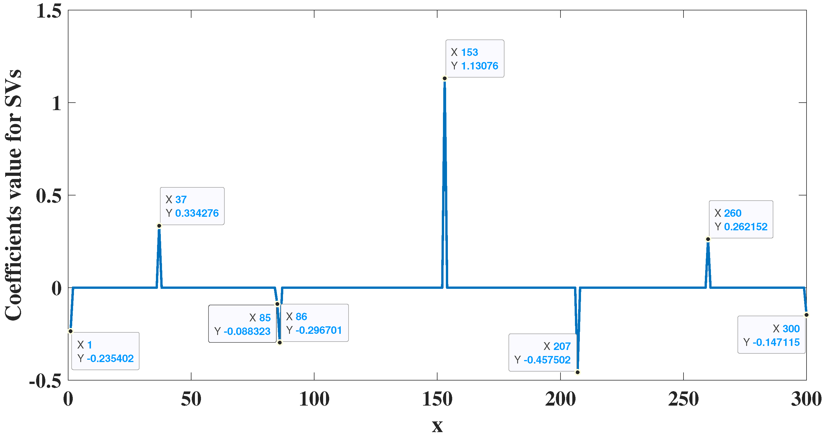
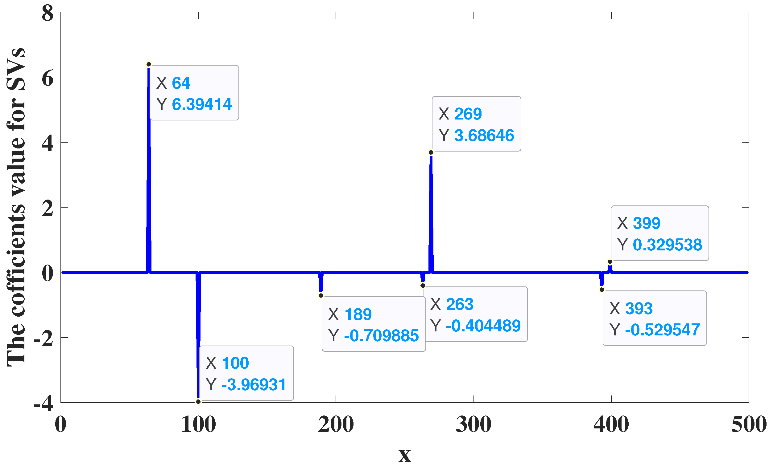
3.2. Kernel Regression Models with Guaranteed Sparsity

The theory of structural risk minimization has been successfully applied to SVR to achieve the sparse nature of the model. However, its sparse property is realized through complex convex optimization theory, Lagrange multiplier methods, and duality principles. In this paper, we first transform the complex quadratic programming in SVR into linear programming to control the complexity of the model structure. Then, we integrate Theorem 1 into the linear programming (12) to form a new optimization problem. This optimization ensures a balance between model accuracy and the complexity of the model structure.

By combining optimization (11) with (18), we obtain the following new optimization problem:

$$\begin{array}{cc}\hfill & min:R\left(f\right)=\gamma ·\sum _{k=1}^N{\xi }_k+\sum _{k=1}^N({\alpha }_k^{+}+{\alpha }_k^{-})\hfill \\ \hfill & +\sum _{k=1}^N{\lambda }_k+b\hfill \\ \hfill & s.t\left\{\begin{array}{c}y\left(k\right)-\sum _{k=1}^N({\alpha }_k^{+}-{\alpha }_k^{-})K(\mathit{x},{\mathit{x}}_k)-b\le {\lambda }_k\hfill \\ -y\left(k\right)+\sum _{k=1}^N({\alpha }_k^{+}-{\alpha }_k^{-})K(\mathit{x},{\mathit{x}}_k)+b\le {\lambda }_k\hfill \\ y\left(k\right)-\sum _{k=1}^N({\alpha }_k^{+}-{\alpha }_k^{-})K(\mathit{x},{\mathit{x}}_k)\hfill \\ -b\le \epsilon +{\xi }_k\hfill \\ \sum _{k=1}^N({\alpha }_k^{+}-{\alpha }_k^{-})K(\mathit{x},{\mathit{x}}_k)+b\hfill \\ -y\left(k\right)\le \epsilon +{\xi }_k\hfill \\ {\xi }_k\ge 0,{\lambda }_k\ge 0,k=1,2,\dots ,N\hfill \end{array}\right.\hfill \end{array}$$

(21)

where the first two inequality constraints are used to ensure the modeling accuracy of the kernel regression model, while the latter two are used to ensure the sparsity of the model. Since the method proposed in this paper is based on SVR, which has a well-established theoretical foundation, the rationality of optimization problem (21) can be ensured. It is clearly seen from Formula (21) that the objective function not only includes the parameter part that controls the model structure, but also incorporates the model accuracy component that dominates the approximation error. The corresponding constraint conditions also reflect the modeling accuracy and sparsity characteristics of the model. To utilize standard linear programming [22], Formula (21) can be expressed in the following vector form:

$$\begin{array}{cc}\hfill & min{\mathbf{c}}^T\left(\begin{array}{c}{\alpha }^{+}\\ {\alpha }^{-}\\ \xi \\ \lambda \\ b\end{array}\right)\hfill \\ \hfill & s.t\left\{\begin{array}{c}\left(\begin{array}{ccccc}\mathit{K}& -\mathit{K}& -\mathbf{I}& \mathbf{Z}& \mathbf{E}\\ -\mathit{K}& \mathit{K}& -\mathbf{I}& \mathbf{Z}& \mathbf{E}\\ -\mathit{K}& \mathit{K}& \mathbf{Z}& \mathbf{Z}& \mathbf{E}\\ \mathit{K}& -\mathit{K}& \mathbf{Z}& -\mathbf{I}& \mathbf{E}\end{array}\right)\left(\begin{array}{c}{\alpha }^{+}\\ {\alpha }^{-}\\ \xi \\ \lambda \\ b\end{array}\right)\\ \le \left(\begin{array}{c}\mathit{y}+\epsilon \\ \epsilon -\mathit{y}\\ -\mathit{y}\\ \mathit{y}\end{array}\right)\\ {\mathit{\alpha }}^{+},{\mathit{\alpha }}^{-}\ge 0,\mathit{\xi }\ge 0,0\le {\mathit{>\lambda }}_{\mathit{k}}\le 1\end{array}\right.\hfill \end{array}$$

(22)

where $\mathit{K}$ represents a matrix, and its elements are computed using the following kernel function:

$$k_{ik}=k({\mathbf{x}}_{\mathbf{i}},{\mathbf{x}}_{\mathbf{k}})=exp(-{\displaystyle \frac{\parallel {\mathbf{x}}_i-{\mathbf{x}}_k{\parallel }^2}{2{\sigma }^2}})$$

and $\sigma$ represents the kernel parameter, which needs to be determined in advance, and

$$\begin{array}{cc}\hfill & \mathbf{c}={(\underset{N}{\underbrace{1,\cdots ,1}},\underset{N}{\underbrace{1,\cdots ,1}},\underset{N}{\underbrace{\gamma ,\cdots ,\gamma }},\underset{N}{\underbrace{1,\cdots ,1}},1)}^T,\hfill \\ \hfill & {\mathit{\alpha }}^{+}={({\alpha }_1^{+},\cdots ,{\alpha }_N^{+})}^T,{\mathit{\alpha }}^{-}={({\alpha }^1-,\cdots ,{\alpha }_N^{-})}^T\hfill \end{array}$$

(23)

$$\begin{array}{cc}\hfill & \mathbf{y}={(y\left(1\right),\cdots ,y\left(N\right))}^T,\mathit{\xi }={({\xi }_1,\cdots ,{\xi }_N)}^T\hfill \\ \hfill & \mathbf{Z}={\mathbf{0}}_{N\times N},\mathbf{E}={\mathbf{1}}_{N\times 1},\mathit{\lambda }={({\lambda }_1,\cdots ,{\lambda }_N)}^T\hfill \end{array}$$

(24)

Finally, we obtain the parameters of the kernel regression model by applying linear programming to solve the new optimization problem. Notably, by solving the optimization (22), we find that the values of the Lagrange multiplier ${\mathit{\alpha }}^{+}$ and ${\mathit{\alpha }}^{-}$ mostly approach zero, which results in the corresponding terms in the kernel regression model (3) being eliminated. This ensures the model’s sparse characteristics. Furthermore, since optimization problem (22) is a classic linear programming problem, the solution obtained is globally optimal.

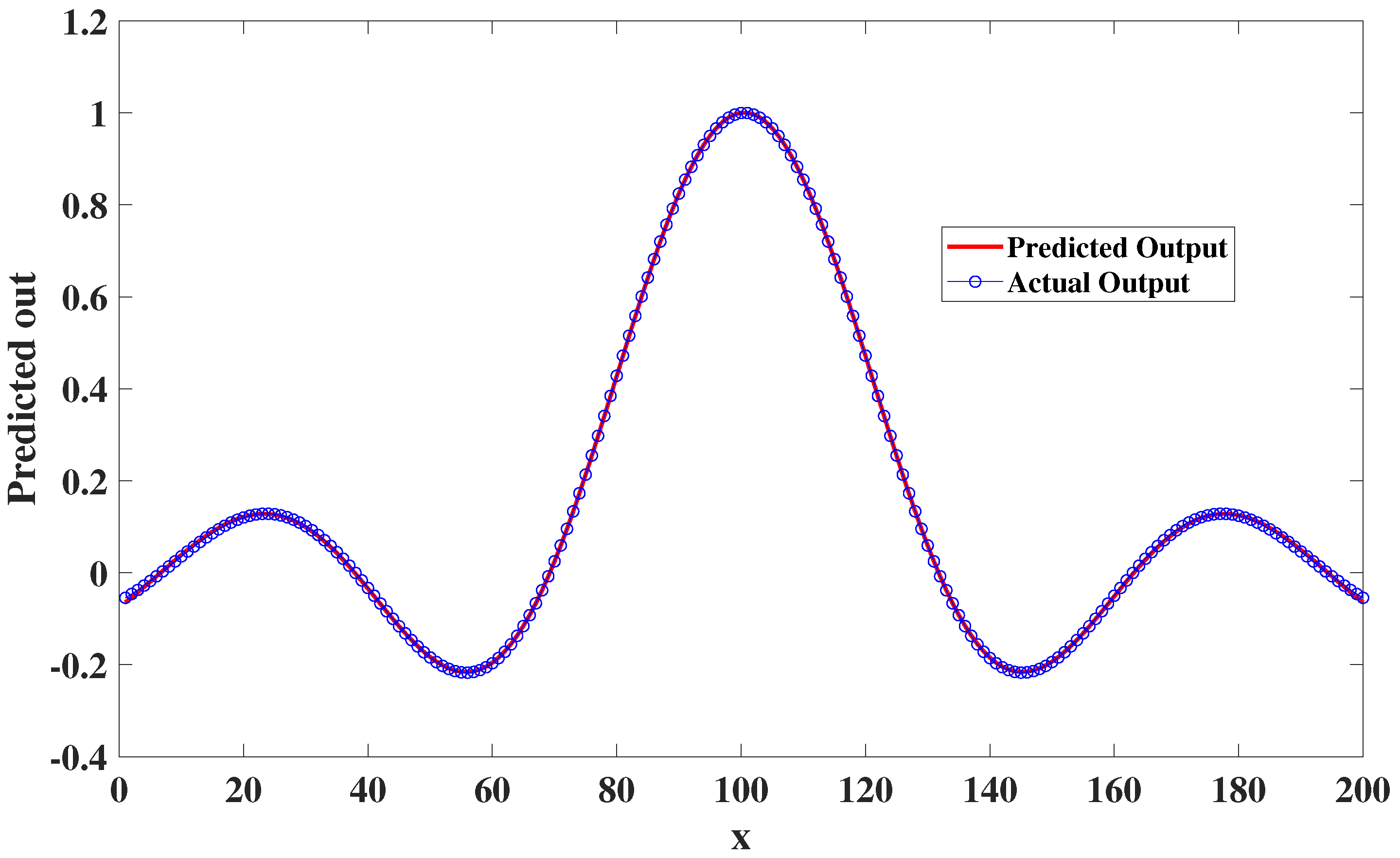
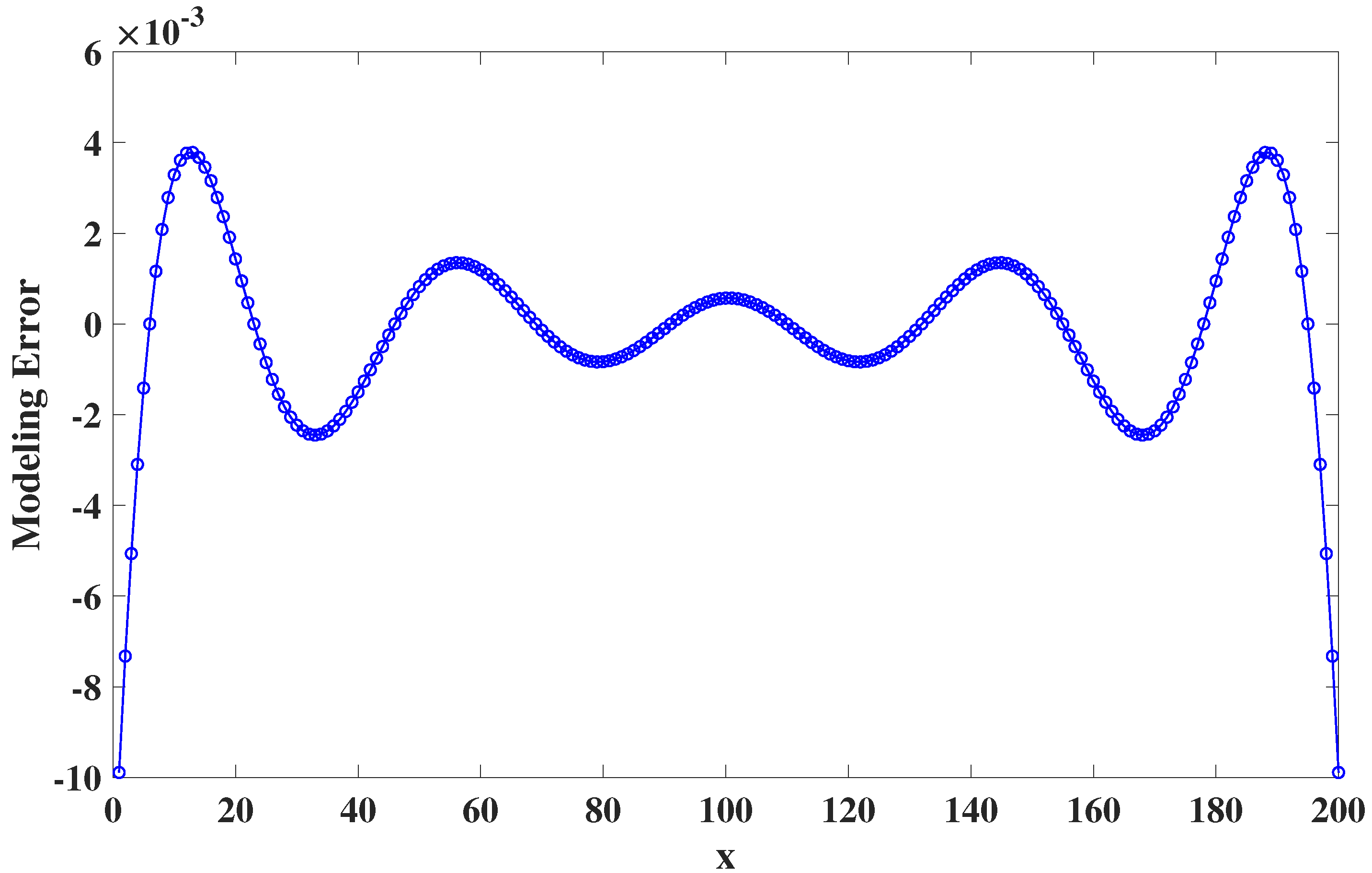
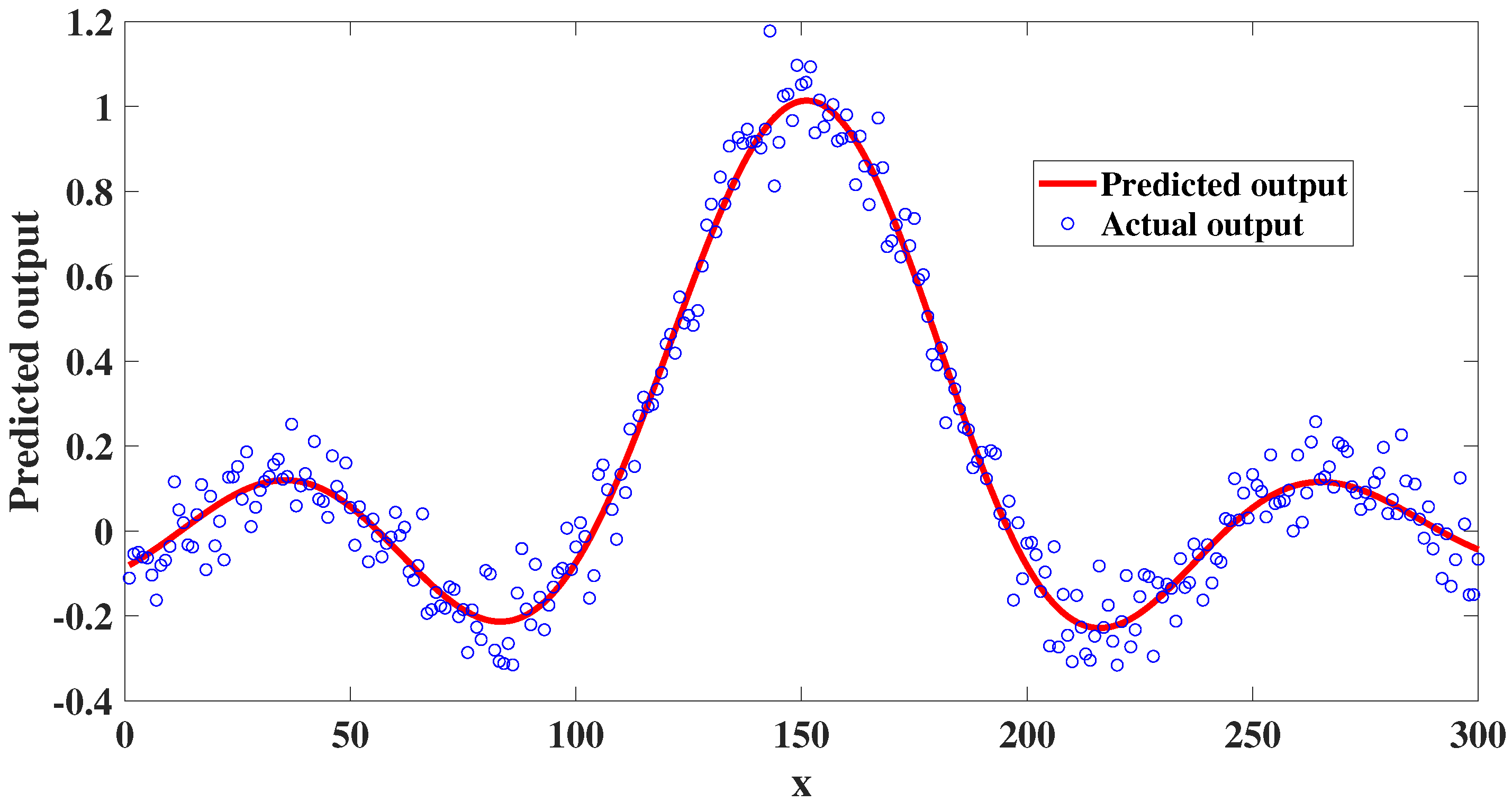
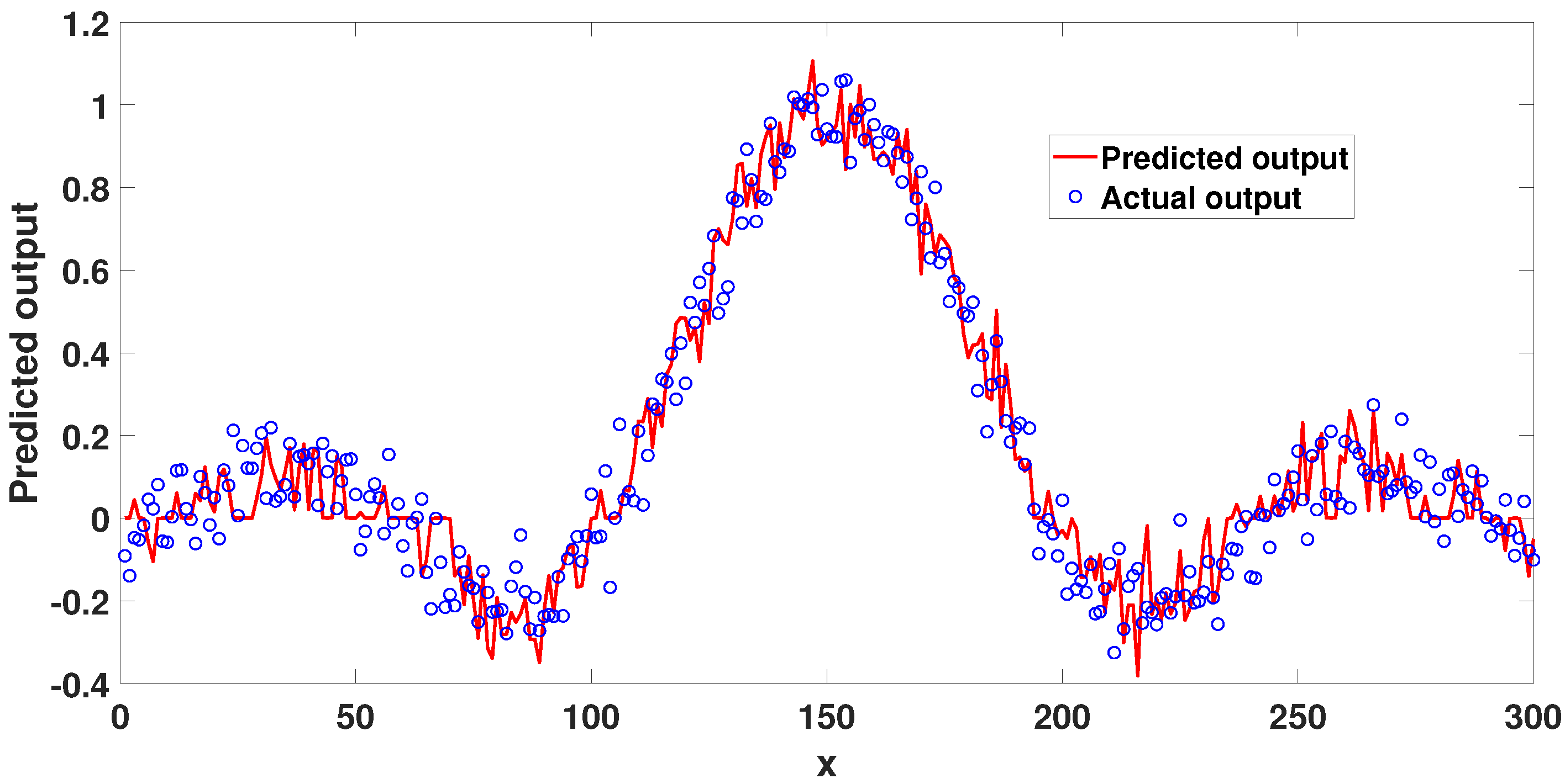
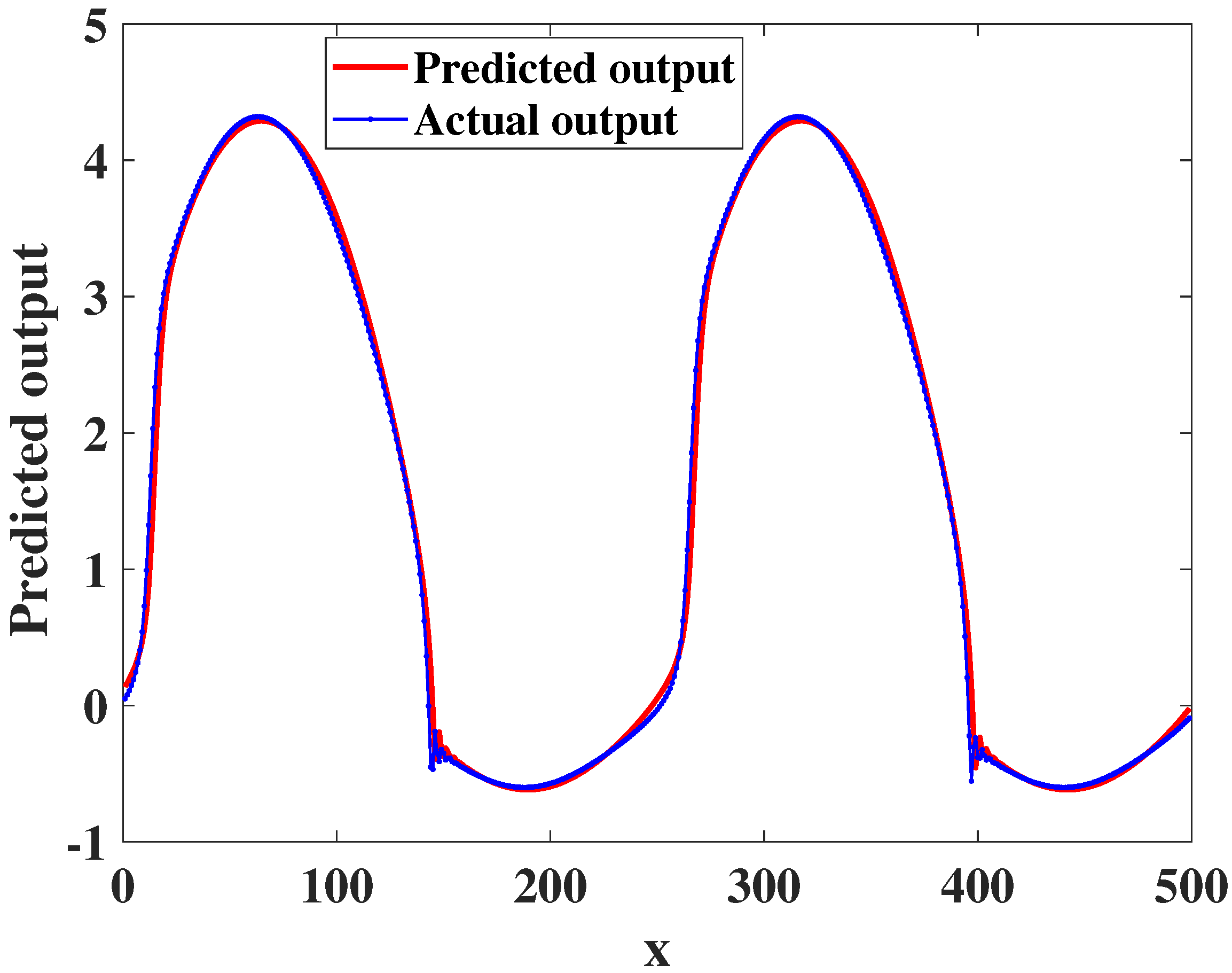
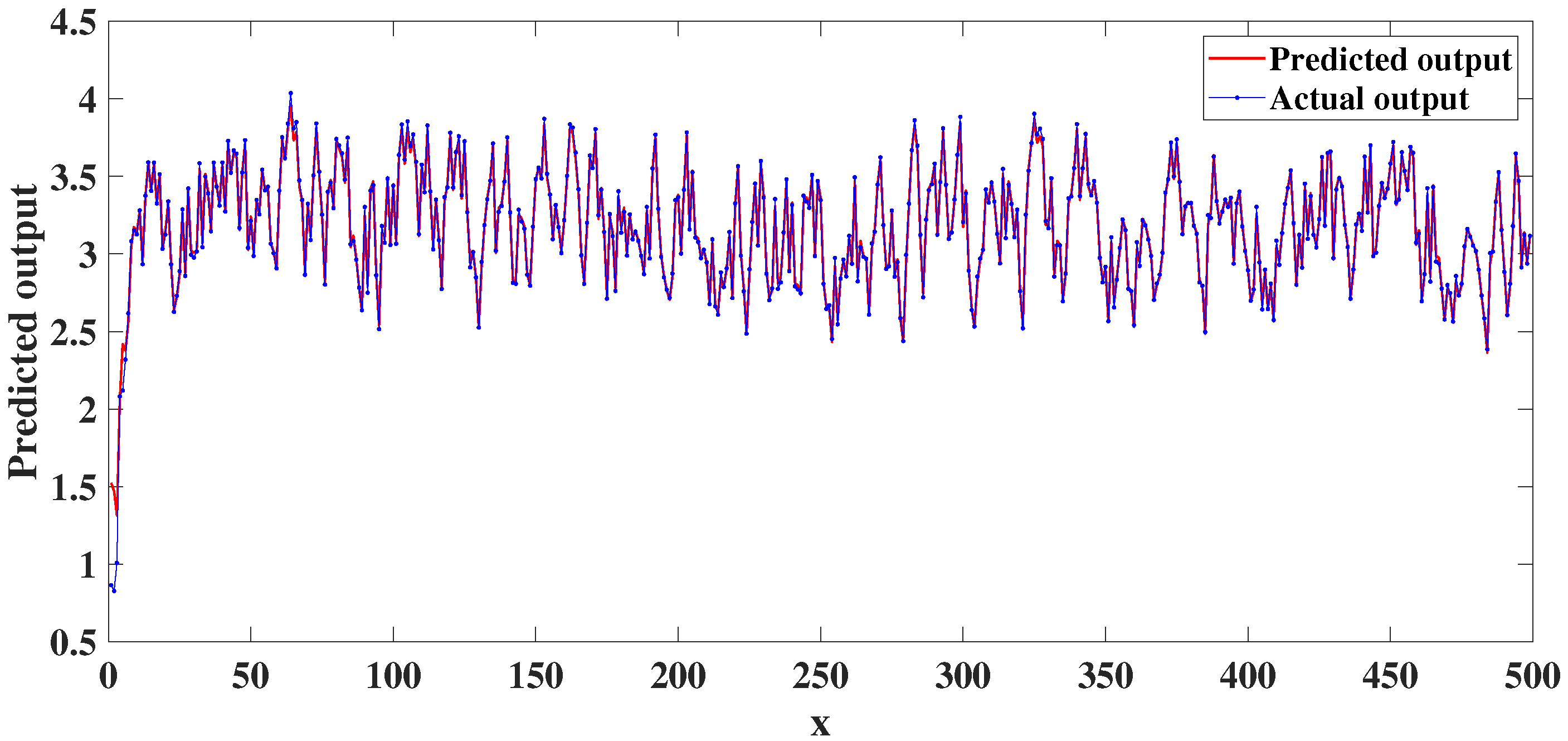
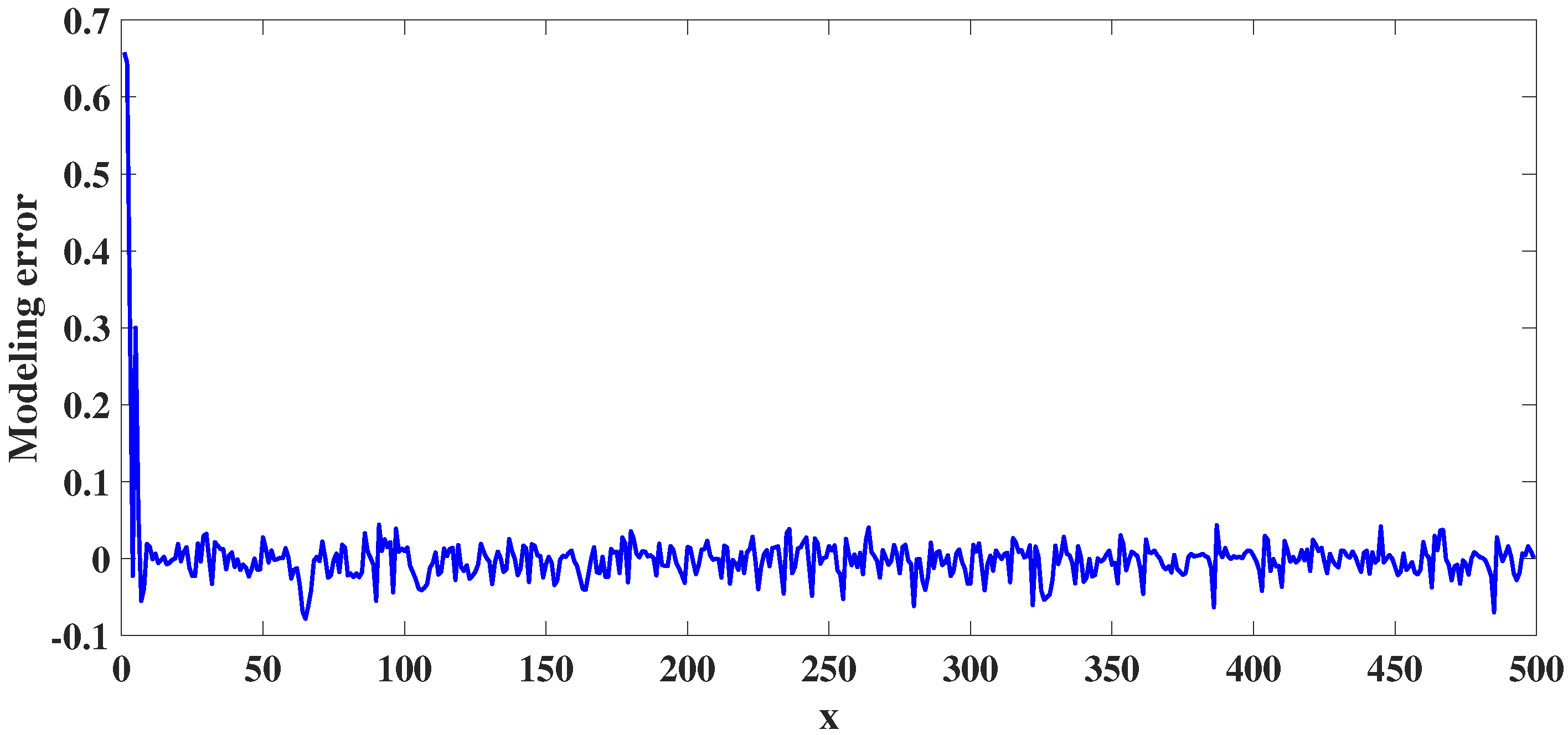
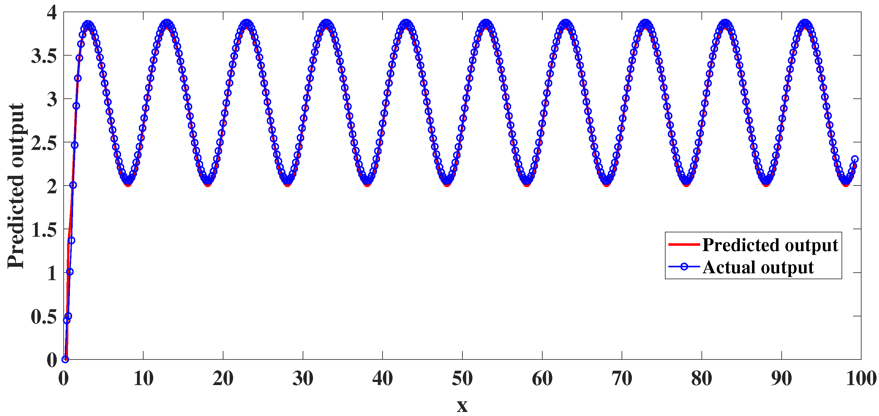
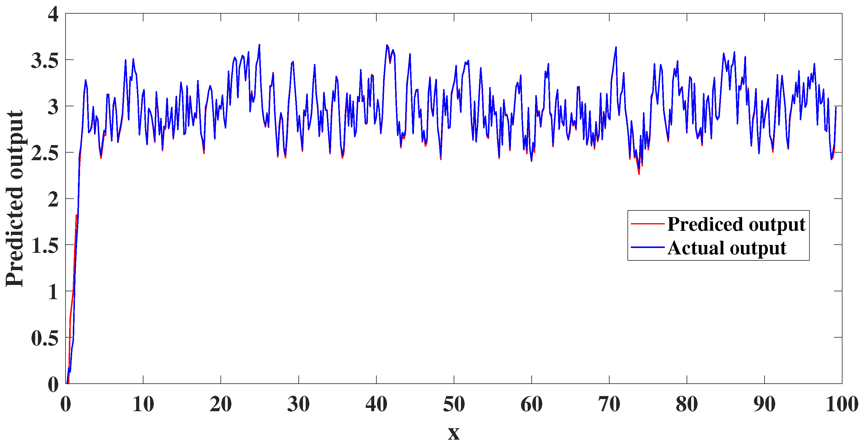
4. Experimental Studies

To demonstrate the effectiveness and superiorities of the proposed method in modeling nonlinear dynamic systems, the following experimental analysis will utilize root mean square error ($RMSE$) and percentage of support vectors ($SVs\%$) as evaluation metrics for validating the performance of the proposed method. $RMSE$ is used to reflect the modeling accuracy of the kernel regression model, while $SVs\%$ is used to evaluate the complexity of the model structure or model sparsity. A smaller $RMSE$ indicates higher modeling accuracy, and the $SVs\%$ corresponds to better sparsity characteristics of the model structure. Obviously, there is a conflict between modeling accuracy and model sparsity. It is necessary to find a balance between both. The following experimental analysis will also further give the relationship between these two aspects. The $RMSE$ is defined as follows:

$$RMSE=\sqrt{{\displaystyle \frac{{\sum }_{k=1}^N{e}_k^2}{N}}}=\sqrt{{\displaystyle \frac{{\sum }_{k=1}^N{(y_k-{\widehat{y}}_k)}^2}{N}}}$$

(25)

where N represents the total amount of test data or training data, $y_k$ is the actual output of a nonlinear static or dynamic system, and ${\widehat{y}}_k$ corresponds to the predicted output of the kernel regression model.

Another important metric is $SVs\%$,

$$SVs\%={\displaystyle \frac{N_k}{N}}\times 100\%$$

(26)

where $N_k$ describes the number of support vectors, which has a decisive impact on the model structure. In the optimization problem of kernel regression models, a sample is considered as a support vector when the magnitude of the coefficient of kernel regression model corresponding to the k-th sample exceeds a certain threshold (this threshold is set to $1\times 1e-8$ in our experiment). Here, N represents the total number of training samples. Strictly speaking, when the condition of $|({\alpha }_k^{+}-{\alpha }_k^{-})|>1e-8$ is satisfied, the corresponding kth sample ${\mathit{x}}_k$ is referred to as a support vector.

4.1. Static Nonlinear System Analysis

Our initial experiment involved utilizing a synthetic dataset that was generated from a commonly selected static nonlinear function $sinc\left(x\right)=sin\left(x\right)/\left(x\right)$ to demonstrate the effectiveness of our methodology. Next, we will demonstrate the proposed method based on the aforementioned two criteria, $RMSE$ and $SVs\%$. First, 200 data points were uniformly generated on the interval [−10 10] for the static nonlinear function without noise interference. When the required hyperparameter set $(\epsilon ,\gamma ,\sigma )$ was selected as (0.01, 100, 2.5), the corresponding kernel regression model and modeling errors are shown in Figure 1 and Figure 2, where $RMSE$ and $SVs\%$ are 0.0020 and 5.0%, respectively. A value of 5.0% for the sparsity measure indicates that only 10 SVs out of the 200 samples were used to build the kernel regression model. This means that those SVs have an important effect on the model. This demonstrates better sparsity (as shown in Figure 3) while ensuring modeling accuracy (as shown in Figure 2) using the proposed method. Considering the relatively small number of support vectors used, we can derive an intuitive expression for the kernel regression model from Figure 4, where X represents the identification number of the support vectors (SV), and Y represents the magnitude of the coefficients. Furthermore, the unmarked coordinates (X, Y) in Figure 4 indicate that the value of Y is equal to 0 or infinitely close to 0, and the corresponding X represents the indices of non-SVs, which play a negligible role in the established kernel regression model.

$$\begin{array}{cc}\hfill f\left(\mathit{x}\right)=& -0.3339·exp\left\{{\displaystyle \frac{{-\parallel \mathit{x}-1\parallel }^2}{2·2.5^2}}\right\}+0.4082·exp\left\{{\displaystyle \frac{{-\parallel \mathit{x}-30\parallel }^2}{2·2.5^2}}\right\}\hfill \\ \hfill & +0.2189·exp\left\{{\displaystyle \frac{{-\parallel \mathit{x}-31\parallel }^2}{2·2.5^2}}\right\}-0.8823·exp\left\{{\displaystyle \frac{{-\parallel \mathit{x}-62\parallel }^2}{2·2.5^2}}\right\}\hfill \\ \hfill & +0.7551·exp\left\{{\displaystyle \frac{{-\parallel \mathit{x}-100\parallel }^2}{2·2.5^2}}\right\}-0.7551·exp\left\{{\displaystyle \frac{{-\parallel \mathit{x}-101\parallel }^2}{2·2.5^2}}\right\}\hfill \\ \hfill & -0.8823·exp\left\{{\displaystyle \frac{{-\parallel \mathit{x}-139\parallel }^2}{2·2.5^2}}\right\}+0.2189·exp\left\{{\displaystyle \frac{{-\parallel \mathit{x}-170\parallel }^2}{2·2.5^2}}\right\}\hfill \\ \hfill & -0.4083·exp\left\{{\displaystyle \frac{{-\parallel \mathit{x}-171\parallel }^2}{2·2.5^2}}\right\}-0.3339·exp\left\{{\displaystyle \frac{{-\parallel \mathit{x}-200\parallel }^2}{2·2.5^2}}\right\}\hfill \end{array}$$

(27)

Actually, when $|{\alpha }_k^{+}-{\alpha }_k^{-}|\ge 1e-8$ was satisfied in our simulation experiments, the corresponding sample is referred to as SV. From the perspective of sparsity and modeling accuracy, the simple example achieved a balance between the two. In addition, it is shown in

Table 1. Comparison results of the different approaches for MSE and $SVs\%$.

Approach	$\mathit{RMSE}$	$\mathit{SVs}\%$
SVR [18]	0.0100	0.3900
RVM [15]	0.0087	0.0900
Literature [23]	0.0030	0.1000
Our approach	0.0020	0.0500

that our approach is superior to other methods in terms of modeling accuracy and model sparsity, where the modeling accuracy $RMSE$ and model sparsity metric $SVs\%$ obtained through our proposed method are 0.0020 and 0.05, respectively, which are significantly better than those of other methods.

Next, we analyze the generalization performance of static nonlinear functions [24] under the influence of zero mean Gaussian noise with a variance of ${\sigma }^2=0.005$.

$$f\left(x\right)=sinc\left(x\right)={\displaystyle \frac{sinx}{x}}+noise$$

(28)

We obtain a training and validation dataset of $N=300$ samples from (28). When the required hyperparameter set $(\epsilon ,\gamma ,\sigma )$ was selected as (0.1, 1000, 2.5), the predicted output of the kernel regression model is shown in Figure 4, where $RMSE$ and $SVs\%$ are 0.0667 and 2.67%, respectively. In other words, the obtained kernel regression model uses only 8 SVs out of the 300 samples and has the better sparsity characteristic, which is described in Figure 5.

Table 2. Comparison of results of the different approaches for $RMSE$ and $SVs\%$.

Approach	Training $\mathit{RMSE}$	Test $\mathit{RMSE}$	$\mathit{SVs}\%$
Literature [24]-P2	0.0832	0.0840	0.0300
Literature [24]-P1	0.0662	0.0693	0.0367
Our approach	0.0667	0.0651	0.0267

gives some results of $RMSE$ and $SVs\%$ in comparison with other approaches, where the proposed method has a better balance between $RMSE$ and $SVs\%$. Although the proposed method has a slightly higher training $RMSE$ in Table 2 compared to that method [24], its sparsity and test accuracy are significantly better. Additionally, when the required hyperparameter set $(\epsilon ,\gamma ,\sigma )$ is selected as (0.1, 1000, 0.1), the predicted output is a non-smooth curve resulting in an overfitting problem, as shown in Figure 6, which indicates that $sinc\left(x\right)$ with noise has a significant detrimental effect on the model. Thus, the occurrence of overfitting must be prevented.

4.2. Dynamic Nonlinear System Analysis

Considering the following dynamic nonlinear system,

$$\begin{array}{cc}\hfill & y(k+1)={\displaystyle \frac{y\left(k\right)y(k-1)\left[y\right(k)+2.5]}{1+y^2\left(k\right)+y^2(k-1)}}+u\left(k\right)\hfill \\ \hfill & y\left(0\right)=y\left(1\right)=0\hfill \end{array}$$

(29)

where $y\left(k\right)$ represents the output at the k-th moment and $u\left(k\right)$ is the known input, for the nonlinear dynamic system, experimental simulations were conducted under two scenarios: without noise and with noise. In the case of no noise, the input signal $u\left(k\right)$ will adopt a sinusoidal signal to obtain the kernel regression model. First, a training and testing dataset of N = 500 samples was generated from Formula (29). If the input–output delay was selected as 2, the training input–output pairs for constructing the kernel regression model were as follows:

$$\begin{array}{cc}\hfill \mathit{x}(k-2)=& \left\{y\right(k-1,y(k-2),u(k-1),u(k-2)\}\hfill \\ \hfill Y(k-2)=& y\left(k\right),k=3,4,\cdots ,N\hfill \end{array}$$

(30)

When the hyperparameter set $(\epsilon ,\gamma ,\sigma )$ was chosen as (0.5, 1000, 6.0), the predicted output of the kernel regression model is shown in Figure 7. The corresponding training and test $RMSE$ values are 0.0696 and 0.0701, and  $SVs\%$ is 1.40%. An $SVs\%$ value of 1.40% indicates that 5 SVs were extracted from the 500 training data points, and the sizes of the coefficients and identification numbers of these SVs in original training data are shown in Figure 8. Evidently, a balance between modeling accuracy and model sparsity has been achieved. Since the number of SVs in Figure 8 is relatively small, we can also write out an intuitive mathematical expression for the kernel regression model.

$$\begin{array}{cc}\hfill f\left(\mathit{x}\right)& =6.3941·exp\left\{{\displaystyle \frac{{-\parallel \mathit{x}-\mathit{x}\left(\mathbf{64}\right)\parallel }^2}{2·1.5^2}}\right\}-3.9693·exp\left\{{\displaystyle \frac{{-\parallel \mathit{x}-\mathit{x}\left(\mathbf{100}\right)\parallel }^2}{2·1.5^2}}\right\}\hfill \\ \hfill & -0.7099·exp\left\{{\displaystyle \frac{{-\parallel \mathit{x}-\mathit{x}\left(\mathbf{189}\right)\parallel }^2}{2·1.5^2}}\right\}-0.4045·exp\left\{{\displaystyle \frac{{-\parallel \mathit{x}-\mathit{x}\left(\mathbf{263}\right)\parallel }^2}{2·1.5^2}}\right\}\hfill \\ \hfill & +3.6865·exp\left\{{\displaystyle \frac{{-\parallel \mathit{x}-\mathit{x}\left(\mathbf{269}\right)\parallel }^2}{2·1.5^2}}\right\}-0.5295·exp\left\{{\displaystyle \frac{{-\parallel \mathit{x}-\mathit{x}\left(\mathbf{393}\right)\parallel }^2}{2·1.5^2}}\right\}\hfill \\ \hfill & +0.3295·exp\left\{{\displaystyle \frac{{-\parallel \mathit{x}-\mathit{x}\left(\mathbf{399}\right)\parallel }^2}{2·1.5^2}}\right\}\hfill \end{array}$$

(31)

where:

$$\begin{array}{cc}\hfill \mathit{x}\mathbf{\left(}\mathbf{64}\mathbf{\right)}=& \left\{y\right(63),y(62),u(63),u(62\left)\right\}\hfill \\ \hfill \mathit{x}\mathbf{\left(}\mathbf{100}\mathbf{\right)}=& \left\{y\right(99),y(98),u(99),u(98\left)\right\}\hfill \\ \hfill \mathit{x}\mathbf{\left(}\mathbf{189}\mathbf{\right)}=& \left\{y\right(188),y(187),u(188),u(187\left)\right\}\hfill \\ \hfill \mathit{x}\mathbf{\left(}\mathbf{263}\mathbf{\right)}=& \left\{y\right(262),y(261),u(262),u(261\left)\right\}\hfill \\ \hfill \mathit{x}\mathbf{\left(}\mathbf{269}\mathbf{\right)}=& \left\{y\right(268),y(267),u(268),u(267\left)\right\}\hfill \\ \hfill \mathit{x}\mathbf{\left(}\mathbf{393}\mathbf{\right)}=& \left\{y\right(392),y(391),u(392),u(391\left)\right\}\hfill \\ \hfill \mathit{x}\mathbf{\left(}\mathbf{399}\mathbf{\right)}=& \left\{y\right(398),y(397),u(398),u(397\left)\right\}\hfill \end{array}$$

(32)

Next, we introduced Gaussian white noise with zero mean and a variance of 0.5 into Formula (29) for an experimental simulation. To enhance the generalization performance of the model, a training input–output dataset of N = 500 samples was obtained by utilizing random signals generated from the interval [0, 1] as inputs. When the hyperparameter set $(\epsilon ,\gamma ,\sigma )$ was chosen as (0.1, 1000, 6), the predicted output and modeling error of kernel regression model are shown in Figure 9 and Figure 10, where the $RMSE$ and $SVs\%$ are 0.0496 and 0.8%, respectively. From Figure 9 and Figure 10 and the training $RMSE$, it can be seen that the modeling accuracy of the kernel regression model using the proposed method is guaranteed. More importantly, the $SVs\%$ accounts for only 0.8%, which means that the number of SVs generated from 300 training samples is only 4. These SVs play a decisive role in establishing the kernel regression model. Figure 11 presents the magnitudes of the coefficients corresponding to SVs and the location numbers of SVs among 300 training samples. It is evident that the superior sparsity characteristic is well-reflected in the proposed method. A mathematical expression for the kernel regression model based on these four SVs can be derived,

$$\begin{array}{cc}\hfill f\left(\mathit{x}\right)=& -10.9829·exp\left\{{\displaystyle \frac{{-\parallel \mathit{x}-\mathit{x}\left(\mathbf{95}\right)\parallel }^2}{2·6^2}}\right\}\hfill \\ \hfill & +26.3704·exp\left\{{\displaystyle \frac{{-\parallel \mathit{x}-\mathit{x}\left(\mathbf{112}\right)\parallel }^2}{2·6^2}}\right\}\hfill \\ \hfill & -0.7851·exp\left\{{\displaystyle \frac{{-\parallel \mathit{x}-\mathit{x}\left(\mathbf{130}\right)\parallel }^2}{2·6^2}}\right\}\hfill \\ \hfill & -11.3811·exp\left\{{\displaystyle \frac{{-\parallel \mathit{x}-\mathit{x}\left(\mathbf{251}\right)\parallel }^2}{2·6^2}}\right\}\hfill \end{array}$$

(33)

where

$$\begin{array}{cc}\hfill \mathit{x}\left(\mathbf{95}\right)=& \left\{y\right(94),y(93),u(94),u(93\left)\right\}\hfill \\ \hfill \mathit{x}\left(\mathbf{112}\right)=& \left\{y\right(111),y(110),u(111),u(110\left)\right\}\hfill \\ \hfill \mathit{x}\left(\mathbf{130}\right)=& \left\{y\right(129),y(128),u(129),u(128\left)\right\}\hfill \\ \hfill \mathit{x}\left(\mathbf{251}\right)=& \left\{y\right(250),y(249),u(250),u(249).\}\hfill \end{array}$$

(34)

The above Formula (33) was used for the validation of the nonlinear dynamic system of (29) under various input signals, including sinusoidal signals, step signals, and random signals. When the input signal $u\left(t\right)$ is a sinusoidal signal, namely,

$$u\left(t\right)=0.5\ast sin(2\ast pi\ast t)+0.5.$$

(35)

comparison results between the actual output and the predicted output obtained by the kernel regression model based on Formula (33) are shown in Figure 12, and the corresponding test $RMSE$ is 0.0614. Furthermore, a step signal was considered as the test input $u\left(t\right)$ in Formula (29), Figure 13 gives the test results using our approach, and the test $RMSE$ is 0.0431. Finally, when the input was a random signal from the interval [0, 1], the obtained test results are shown in Figure 14 with a $RMSE$ of 0.8. Through the experimental analysis of static and dynamic nonlinear systems, we have found that the optimization problem of solving a kernel regression model can guarantee the modeling accuracy and sparsity characteristics of the model well. Therefore, our method further enhances the generalization performance of the model.

5. Conclusions

Traditional modeling methods are prone to over-fitting issues, resulting in unsatisfactory results in practical applications. In this paper, we transform the complex convex quadratic problem into a simple optimization only involving $L_1$-norm. It combines the $L_1$-norm of the approximation error with the $L_1$-norm optimization that can control the complexity of the model structure well to form a new optimization problem. A simpler linear programming is adopted to solve parameters of the kernel regression model. The resulting model achieves good balance between modeling accuracy and sparsity characteristics and enhances the generalization performance of the model. Finally, through experimental simulations on static and dynamic nonlinear systems, the proposed method was validated.

References

1. Zhong, X.; Song, R.; Shan, D.; Ren, X.; Zheng, Y.; Lv, F.; Deng, Q.; He, Y.; Li, X.; Li, R.; et al. Discovery of hepatoprotective activity components from Thymus quinquecostatus celak. by molecular networking, biological evaluation and molecular dynamics studies. Bioorg. Chem. 2023, 140, 106790. [Google Scholar] [CrossRef]
2. Yan, J.; Nuertayi, A.; Yan, Y.; Liu, S.; Liu, Y. Hybrid physical and data driven modeling for dynamic operation characteristic simulation of wind turbine. Renew. Energy 2023, 215, 118958. [Google Scholar] [CrossRef]
3. Zhang, D.; Bhattarai, H.; Wang, F.; Zhang, X.; Hwang, H.; Wu, X.; Tang, Y.; Kang, S. Dynamic characteristics of segmental assembled HH120 wind turbine tower. Renew. Energy 2024, 303, 117438. [Google Scholar] [CrossRef]
4. Pham, M.; Nguyen, M.; Bui, T. A novel thermo-mechanical local damage model for quasi-brittle fracture analysis. Theor. Appl. Fract. Mech. 2024, 130, 104329. [Google Scholar] [CrossRef]
5. Toffolo, K.; Meunier, S.; Ricardez-Sandoval, L. Reactor network modelling for biomass-fueled chemical-looping gasification and combustion processes. Fuel 2024, 366, 131254. [Google Scholar] [CrossRef]
6. Sadeqi, A.; Moradi, S.; Heidari Shirazi, K. Nonlinear subspace system identification based on output-only measurements. J. Frankl. Inst. 2020, 357, 12904–12937. [Google Scholar] [CrossRef]
7. Sadeqi, A.; Moradi, S. Nonlinear system identification based on restoring force transmissibility of vibrating structures. Mech. Syst. Signal Process. 2022, 172, 108978. [Google Scholar] [CrossRef]
8. Meng, X.; Zhang, Y.; Quan, L.; Qiao, J. A self-organizing fuzzy neural network with hybrid learning algorithm for nonlinear system modeling. Inf. Sci. 2023, 642, 119145. [Google Scholar] [CrossRef]
9. Han, H.; Guo, Y.; Qiao, J. Nonlinear system modeling using a self-organizing recurrent radial basis function neural network. Appl. Soft Comput. 2018, 71, 1105–1116. [Google Scholar] [CrossRef]
10. Wei, C.; Li, C.; Feng, C.; Zhou, J.; Zhang, Y. A t-s fuzzy model identification approach based on evolving mit2-fcrm and wos-elm algorithm. Eng. Appl. Artif. Intell. 2020, 92, 103653. [Google Scholar] [CrossRef]
11. Goethals, I.; Pelckmans, K.; Suykens, J.; Moor, B. Subspace identification of hammerstein systems using least squares support vector machines. IEEE Trans. Autom. Control 2005, 50, 1509–1519. [Google Scholar] [CrossRef]
12. Pilario, K.; Cao, Y.; Shafiee, M. A kernel design approach to improve kernel subspace identification. IEEE Trans. Ind. Electron. 2021, 68, 6171–6180. [Google Scholar] [CrossRef]
13. Rigatos, G.; Tzafestas, G. Extended Kalman filtering for fuzzy modelling and multi-sensor fusion. Math. Model. Syst. 2007, 13, 251–266. [Google Scholar] [CrossRef]
14. Lei, Y.; Xia, D.; Erazo, D.; Nagarajaiah, S. A novel unscented kalman filter for recursive state-input-system identification of nonlinear systems. Mech. Syst. Signal Process. 2019, 127, 120–135. [Google Scholar] [CrossRef]
15. Tipping, M. Sparse bayesian learning and the relevance vector machine. J. Mach. Learn. Res. 2001, 1, 211–244. [Google Scholar]
16. Li, Y.; Luo, Y.; Zhong, Z. An active sparse polynomial chaos expansion approach based on sequential relevance vector machine. Comput. Methods Appl. Mech. Eng. 2024, 418, 116554. [Google Scholar] [CrossRef]
17. Vapnik, V. The support vector method. In International Conference on Artificial Neural Networks; Springer: Berlin/Heidelberg, Germany, 1997; pp. 261–271. [Google Scholar]
18. Smola, A.; Bernhard, S. A tutorial on support vector regression. Stat. Comput. 2004, 14, 199–222. [Google Scholar] [CrossRef]
19. Ucak, K.; Oke Gunel, G. Adaptive stable backstepping controller based on support vector regression for nonlinear systems. Eng. Appl. Artif. Intell. 2024, 129, 107533. [Google Scholar] [CrossRef]
20. Han, S.; Lee, S. Recurrent fuzzy neural network backstepping control for the prescribed output tracking performance of nonlinear dynamic systems. ISA Trans. 2014, 53, 33–43. [Google Scholar] [CrossRef]
21. Warwicker, J.; Rebennack, S. Support vector machines within a bivariate mixed-integer linear programming framework. Expert Syst. Appl. 2024, 245, 122998. [Google Scholar] [CrossRef]
22. Aharon, B.; Nemirovski, A. Robust solutions of linear programming problems contaminated with uncertain data. Math. Program. 2000, 88, 411–424. [Google Scholar]
23. Liu, X.; Fang, H. Kernel regression model guaranteed by identifying accuracy and model sparsity for nonlinear dynamic system identification. Sci. Technol. Eng. 2020, 20, 7804–7814. [Google Scholar]
24. Manngrd, M.; Kronqvist, J.; Bling, J. Structural learning in artificial neural networks using sparse optimization. Neurocomputing 2018, 272, 660–667. [Google Scholar] [CrossRef]
Figure 1. Predicted output of kernel regression model using proposed method.
Processes 12 02358 g001
Figure 2. Modeling error for sparse kernel regression model.
Processes 12 02358 g002
Figure 3. Coefficient values and corresponding identification numbers for SVs.
Processes 12 02358 g003
Figure 4. Predicted output of kernel regression model using proposed method.
Processes 12 02358 g004
Figure 5. Coefficient values and corresponding identification numbers for SVs.
Processes 12 02358 g005
Figure 6. Predicted output of kernel regression model using proposed method with overfitting.
Processes 12 02358 g006
Figure 7. Predicted output of kernel regression model using proposed method.
Processes 12 02358 g007
Figure 8. Coefficient values and corresponding identification numbers for SVs.
Processes 12 02358 g008
Figure 9. Predicted output of kernel regression model using proposed method.
Processes 12 02358 g009
Figure 10. Modeling error for kernel regression model.
Processes 12 02358 g010
Figure 11. Coefficient values and corresponding identification numbers for SVs.
Processes 12 02358 g011
Figure 12. Predicted output of kernel regression model using proposed method.
Processes 12 02358 g012
Figure 13. Predicted output of kernel regression model using proposed method.
Processes 12 02358 g013
Figure 14. Predicted output of kernel regression model using proposed method.
Processes 12 02358 g014