An Enhanced Fault Localization Technique for Distribution Networks Utilizing Cost-Sensitive Graph Neural Networks

Abstract

Accurate and timely fault diagnosis is of great significance for the stable operation of a distribution network. Traditional artificial intelligence-based localization methods rely heavily on large-scale labeled datasets, making them prone to being affected by distributed generators. To address this issue, this study proposes a fault location method for distribution systems using a cost-sensitive graph attention network model. In this approach, the physical structure of the distribution network is considered a crucial constraint for model training, thereby enhancing its information perception capabilities. Specifically, the electrical nodes and lines of the distribution network are mapped to the vertices and edges within the graph attention network, with the attention weights determined by the correlation of adjacent node fault characteristics, thus improving the sensitivity to grounding faults. Additionally, a cost-sensitive matrix is used to balance class distribution, enhancing the robustness and generalization ability of the model. Fault localization experiments were conducted on the IEEE-33 bus distribution system to validate the effectiveness of the proposed fault localization method. Factors such as data disturbance, varying fault grounding resistances, and distributed power supply access were employed to assess the model’s anti-interference performance. The experimental results demonstrate that the fault location method exhibits high positioning accuracy and excellent robustness.

1. Introduction

Single-phase grounding is a common fault in distribution networks, and small current grounding faults are difficult to detect promptly because they do not disrupt the continuous supply of electricity. However, if the distribution network is in a faulty state for a long time, it may evolve from a single-phase grounding fault to an interphase short-circuit fault, resulting in power safety accidents [1]. Therefore, studying fault diagnosis techniques for distribution networks to locate quickly the point of fault occurrence is of great significance for the safe operation of distribution networks.

Fault location in distribution networks is a prerequisite for fault isolation and power supply recovery, which plays an important role in improving power quality and reducing the power outage range. There are two methods for fault localization, i.e., utilizing fault information uploaded by the feeder terminal unit (FTU) [2], and applying fault current characteristics. Among them, the FTU information-based method mainly includes the matrix method [3,4] and the intelligent optimization method [5,6,7,8,9]. The matrix method generates a fault information matrix according to the FTU information, combines a grid description matrix to obtain a fault judgment matrix, and locates the fault segment according to the fault judgment criterion. This method only utilizes the node information associated with the fault segment, which has advantages such as low computational complexity and fast localization speed. However, it suffers from low fault tolerance, especially when the distribution network is connected to distributed generation (DG). The intelligent optimization method is based on the minimum fault diagnosis set, gradually approaching the fault segment, such as the genetic algorithm [5,6], bat algorithm [7], particle swarm algorithm [8], and immune algorithm [9,10]. This method has good fault tolerance, but the solving process is complicated, and the fault location efficiency of distribution networks is unsatisfied. The fault location method based on fault current characteristics is mainly based on the polarity and similarity of the zero-sequence current to complete the fault segment localization. Ref. [11] performs modal decomposition on the transient zero-sequence current uploaded by the FTU on the feeder during a single-phase ground fault and employs the positive and negative values of the product of the differences between adjacent detection points to determine the fault segment. Ref. [12] constructs a fundamental zero-sequence current fault direction measurement and establishes the multi-index optimization model for fault direction measurement. Ref. [13] adopts the injection signal method to control the neutral point voltage for amplifying the fault characteristics and to compare the steady-state value of the zero-sequence current amplitude with the threshold value to locate the fault segment. These above methods utilize the network structure information and fault features to solve the fault location task, but the weak feature extraction ability and the complex analysis process limit the localization performance.

The artificial intelligence method provides a new path for mapping fault features to fault locations, which allows for the nonlinear mapping of complex inputs and expected outputs without system dynamic information [14]. In general, the machine learning methods applied in fault diagnosis include support vector machines [15], K-nearest neighbors [16], decision trees [17], artificial neural networks [18], and convolutional neural networks [19,20]. Ref. [19] performs spectrum analysis to extract voltage signal features and analyzes the first 100 harmonics of the voltage signal by neighboring components to obtain additional information features. Due to the lack of current data, the measurement error in calculation and CT saturation in short-circuit faults are reduced, but the fault location cannot be determined by this method. Ref. [20] uses a long short-term memory (LSTM) model for fault detection, which can be trained only with data collected from a limited number of phasor measurement units (PMUs) in the network.

In recent years, the graph neural network (GNN) extended neural network methods to the graph domain, achieving the combination of deep learning and graph data [21]. Currently, graph convolutional network (GCN) and graph attention network (GAT) have been applied in power systems. Refs. [22,23] apply the GCN for fault prediction in distribution networks, fully considering the connections between nodes and greatly improving the fault prediction accuracy. Ref. [24] employs the GCN to construct a fault location framework for distribution networks, combining measured values at different nodes with network topology to achieve high discrimination accuracy. Different from the GCN, the GAT introduces an attention mechanism that focuses more on neighboring nodes [25]. The GAT model has proved its strong generalization ability in many fields, but its application in the field of power systems is still in its early stages.

Meanwhile, the integration of DGs adds additional complexity to distribution networks. The presence of DGs increases the number of fault propagation paths and alters fault current and voltage levels, making it difficult for conventional fault location algorithms to adapt rapidly their threshold settings and decision criteria. Moreover, traditional AI-based fault location methods require large-scale labeled datasets for training, which leads to significantly increased costs for data collection and labeling in distribution networks with distributed power generation. The impact of DGs on faults also varies depending on the penetration rate, necessitating that fault location algorithms possess strong generalization capabilities to maintain good positioning performance under continuously changing conditions of DGs.

This study aimed to use GAT to establish a fault location model suitable for distribution networks, considering the influence of network topology and adjacent nodes from a spatial perspective. Meanwhile, a cost-sensitive loss function was designed to improve classification accuracy and reduce generalization errors. The model performance was verified by building a simulation model for small current grounding faults in distribution networks. The results showed that the cost-sensitive GAT model is suitable for fault localization tasks in distribution networks with frequent topology changes. The main contributions of this study are outlined below.

A novel fault localization model based on deep graph learning is proposed and related fault localization experiments were conducted based on the IEEE 33-node distribution system. The graph structure was constructed according to the structural relationship of the measured data from the physical distribution network. The graph-based method can embed topological information into the learning process of the model, enabling the model to learn deeper data structure information and adapt to abnormal data and changes in conditions.

The attention mechanism-based GAT calculates attention weights according to the correlation of adjacent node fault characteristics. By adopting the multi-head attention mechanism, each attention head may learn slightly different focuses, which can more effectively mine deep-level features and improve the stability of the model.

The cost-sensitive matrix was introduced to balance the class distribution and improve the performance and generalization ability of the diagnosis model. The loss function assigned different weights to different categories of samples, so that the model pays more attention to the categories with higher weights in the training process, thereby improving the classification performance.

The remainder of this paper is organized as follows. Section 2 discusses the impact of DGs on fault location in distribution networks. Section 3 shows the proposed distribution network fault location model based on a cost-sensitive graph attention network, including the theoretical basis and technical details of the implementation. Section 4 verifies the effectiveness of the proposed model through case studies. Section 5 presents the conclusion of this study.

2. Distribution Network System with Distributed Power Sources

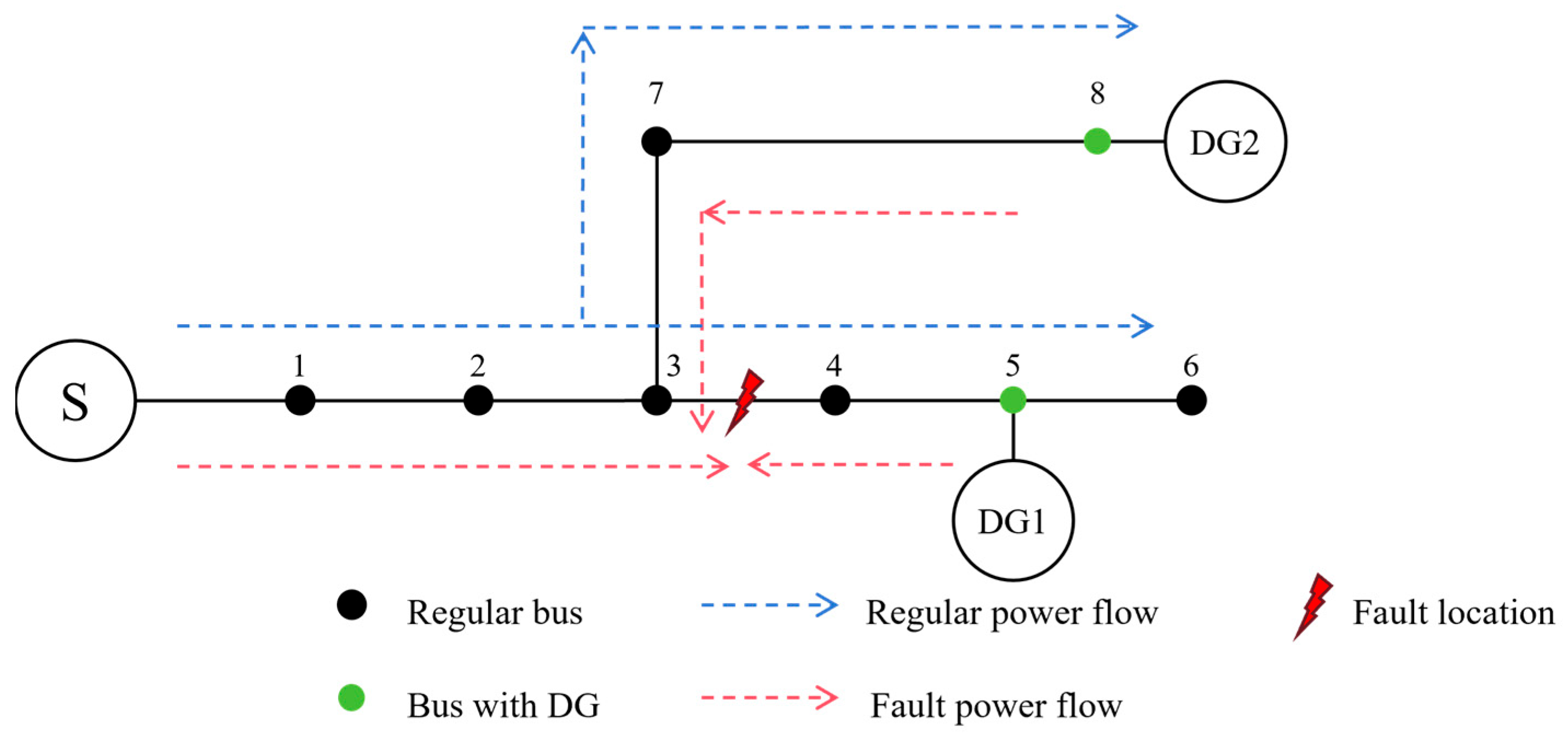
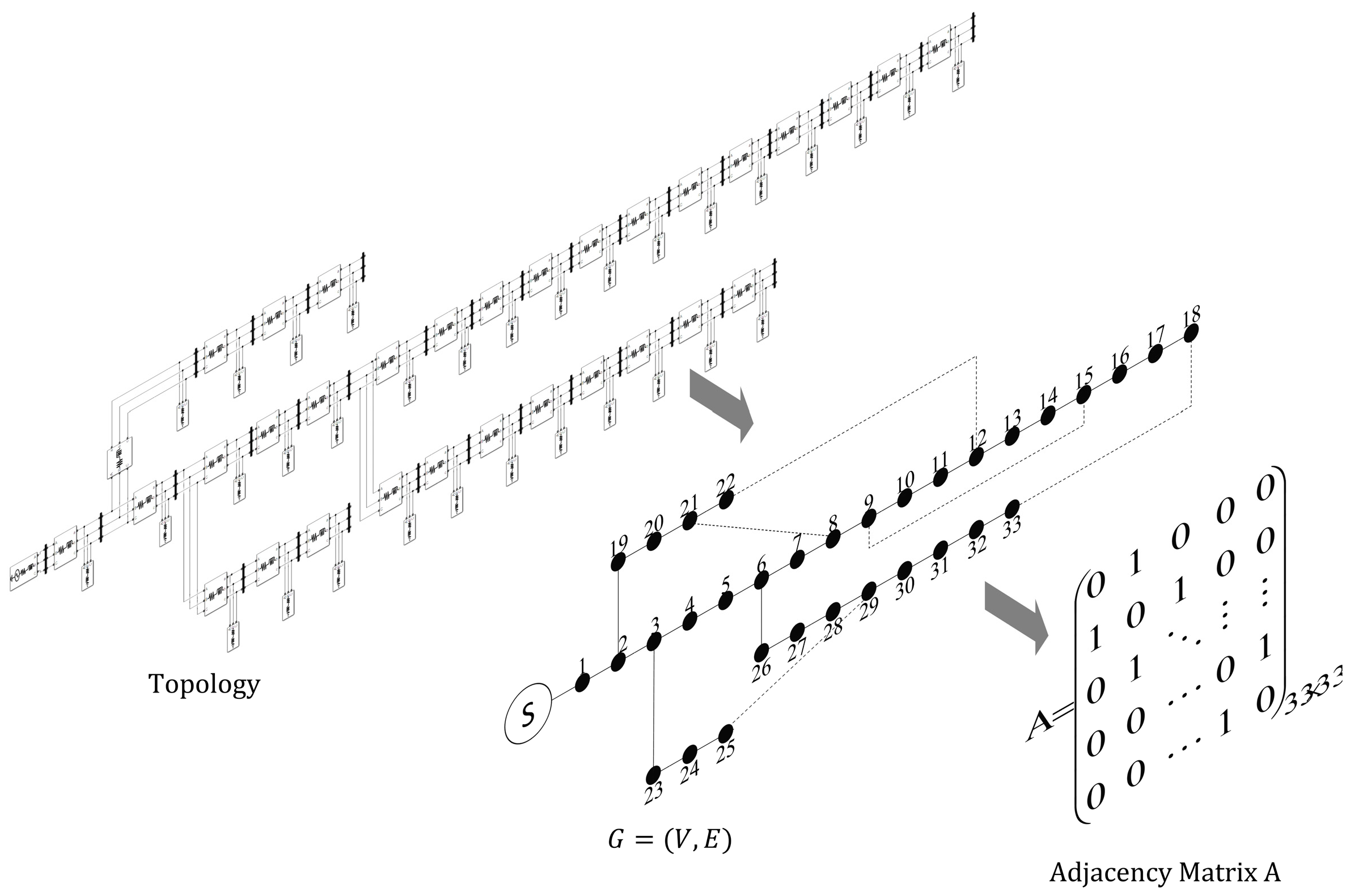
2.1. Typical Distribution Network System

With the expansion of distribution network capacity and scale, as well as the integration of DG and diversified loads, the distribution network has changed from the passive state to the active state, and the power flow has changed from unidirectional to bidirectional. This will affect the structure and load characteristics of the distribution network, increase the difficulty of voltage control, reduce the level of power quality, and lead to an increase in the complexity and control difficulty of the active distribution network.

When distributed power sources are not connected, the active and reactive power consumed by each node load in the distribution network line is positive, and the node voltage gradually decreases along the direction of the line flow. When distributed power sources are connected, the distribution network changes from active to passive, and the power flow changes from single-phase to bidirectional, making it difficult to predict the direction and magnitude of the power flow. In addition, the integration of distributed power sources has an increasing effect on the voltage at the connection location and the end of the line, and the magnitude of the voltage increase is related to the capacity of the DG.

Figure 1 shows the IEEE-33 bus distribution network, where distributed photovoltaics with a capacity of 1 MW are connected at terminal nodes 18 and 33. The simulation model is constructed by MATLAB/Simulink, and the parameters, such as node loads, branch impedance, etc., in the model are mainly referred to reference [26], while the voltage variations at all nodes are shown in Figure 2a, and the current variations are shown in Figure 2b.

As shown in Figure 2, the node voltage becomes the maximum value in the local area after the DG connection, and the voltage of other nodes on the line also increases to varying degrees. Specifically, the magnitude of voltage rise is more pronounced at nodes closer to the end of the line (such as nodes 18 and 33). Meanwhile, the access of DGs can provide current to the upstream branch of the access location, reducing or even increasing the upstream current level of the access location in the opposite direction.

As presented in Figure 2b, the power flow direction of the distribution system changes at nodes 18 and 33 after the DG connection. Therefore, the current direction at nodes 7–18 and 26–30 is opposite to that without the DG connection. It can be observed that the current level of nodes 1–7 decreased significantly after DG was connected, while nodes 19–22 and 23–25 were almost unaffected. Moreover, when nodes 18 and 33 are simultaneously connected to the DG, the penetration rate of the DG is further improved. Compared to connecting a single DG, the current level of upstream nodes at the connection location is further reduced.

2.2. Distribution Network Fault Simulation

Although the integration of distributed power sources can enhance line voltages and reduce transmission losses, it also complicates the structure of distribution networks. This complexity introduces multiple directions of power flow, reducing the security of overcurrent protection. Consequently, there is an increased risk of maloperation or failure of protection devices, which directly impacts the safe and reliable operation of the distribution network.

When a short-circuit fault occurs in the traditional distribution network, the current will significantly increase. However, when the DG is connected to the grid, the direction of the distribution network flow will change, and the fault current will also change accordingly. Figure 3 shows the variation of power flow in the distribution network after connecting to the DG, which depends on factors such as the location and capacity of the DG connection, as well as the distance from the fault point.

When the short-circuit fault occurs between node 2 and node 3, DG1 and DG2 are both downstream of the fault point, providing reverse short-circuit current to the fault point and drawing the short-circuit current provided by the system power supply S, further reducing the forward short-circuit current and causing the protection device to not operate. This makes it difficult to locate the fault in a timely manner, and prolonged failure operation will expand the scope of the fault. When a short-circuit fault occurs between node 3 and node 4, DG2 and the system power supply S together provide a short-circuit current to the fault point, while DG1 provides a reverse fault current to the fault point after the fault point. If the DG capacity is large and the short-circuit current exceeds the set value of the protection device, the FTU at nodes 7, 8, and 4 will detect the reverse fault current, which may affect the accuracy of the fault location. When the short-circuit fault occurs between node 5 and node 6, DG1 and DG2 simultaneously supply power to the short-circuit point, which contributes to an increase in the short-circuit current. The FTU at nodes 7 and 8 may detect reverse current, but the fault location method is less affected.

In summary, when the DG is connected upstream of the fault segment, it will provide a reverse fault current to the short-circuit point, weakening the fault current. When the fault segment is connected downstream of the DG, the DG provides a forward fault current to the fault point, which helps to increase the fault current. When the DG access location is not in the branch of the fault segment, the DG provides fault current to the fault point through the branch, and the node on the branch where the DG is located will detect the reverse fault current. If the DG access capacity is small, it will affect the voltage and current levels of the nodes, thereby changing the distribution of power flow, resulting in a decrease in FTU sensitivity and errors or omissions in fault information. Therefore, it is urgent to establish a new fault location method suitable for distributed power grid connection conditions.

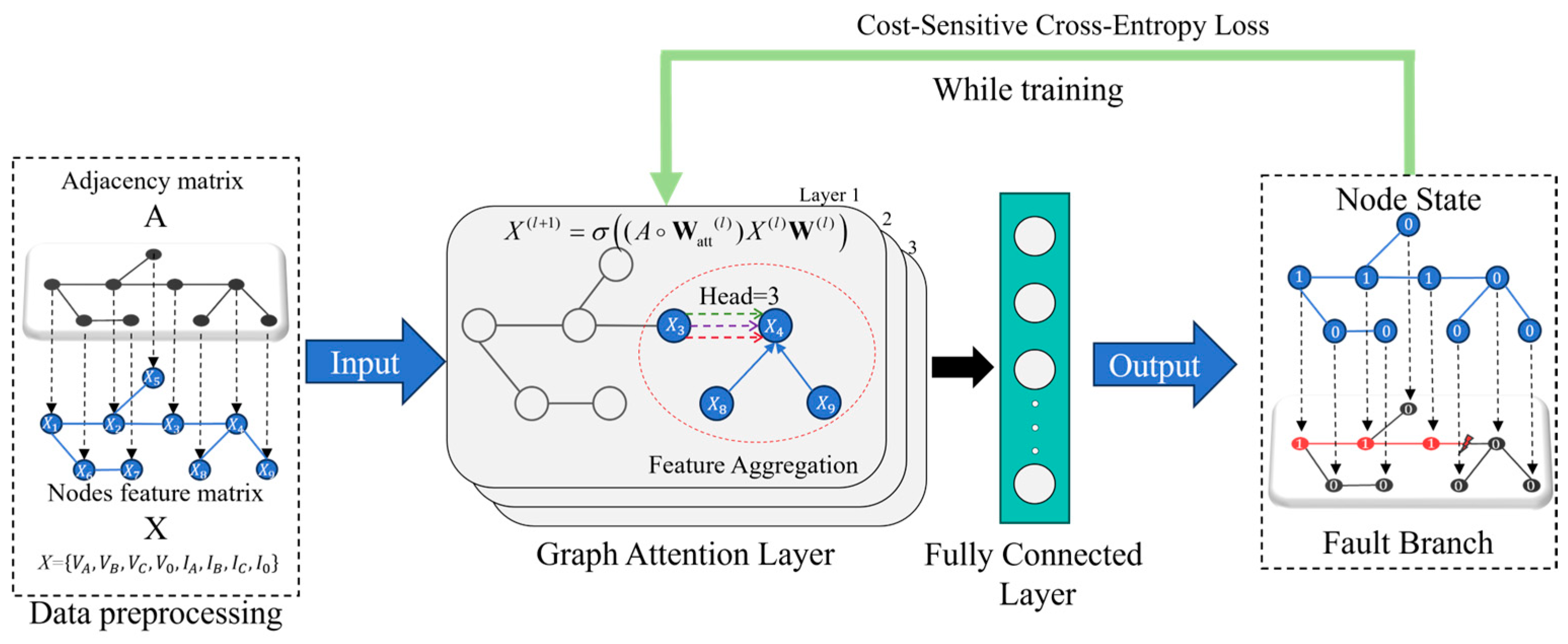
3. Cost-Sensitive Graph Attention Mechanism

The problem of fault location in distribution networks can be seen as a fault state classification problem, which distinguishes whether different nodes are in a fault state or in a normal operating state. GCN can combine the graph information of the distribution network topology and the electrical information of each node to determine each node state, thereby achieving accurate fault localization. Unlike the GCN, the GAT can utilize attention mechanisms to pay more attention to neighbor nodes, which is more suitable for the distribution network branch and the node changes. The fault location model based on the graph attention network proposed in this study is shown in Figure 4.

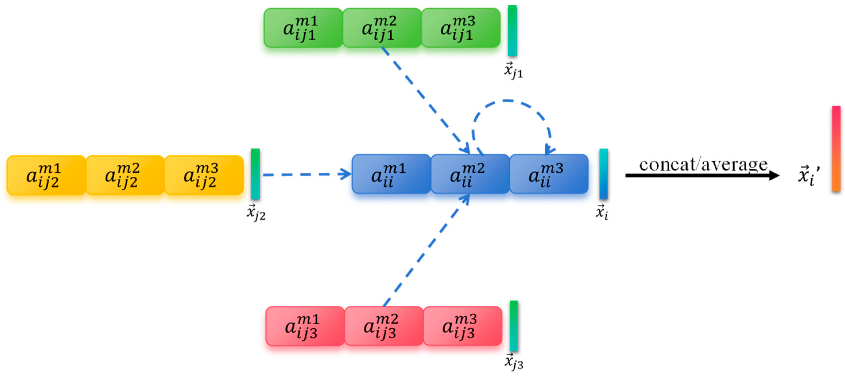
3.1. Graph Attention Network

The GAT propagates hierarchically by aggregating graph structure information and node feature information, namely the following:

$$X^{(l+1)}=\sigma \left(\left(A\circ {W_{att}}^{\left(l\right)}\right)X^{\left(l\right)}{W}^{\left(l\right)}\right)$$

(1)

where $X$ is the node feature matrix, $\sigma$ is the ReLU activation function, $A$ is the adjacency matrix of the graph, $W_{att}$ is the attention coefficient matrix, and $W$ is the weight matrix. Although both GCN and GAT aggregate the features of the neighbor nodes onto the central node, the GCN constructs a Laplacian matrix to participate directly in the calculation of the adjacency matrix $A$, and its neighboring nodes share weights. From the perspective of the spatial domain, the GAT employs the adjacency matrix to determine the connection relationship between nodes, adaptively aggregates the neighbor node information according to different weight coefficients through the attention mechanism, and better integrates the correlation of distribution network node features into the fault location model. The mathematical form of the attention mechanism can be expressed as follows:

$$Attention(Q,S)=\sum _i^{\mathrm{P}}<Q,S_i>· S_i$$

(2)

where $P$ is the total amount of information, $Q$ is the known information, $S$ is the information to be processed, $<Q,S_i>$ represents the inner product operation of the i-th information in $Q$ and $S$ to obtain their correlation degree. For the graph information, $Q$ is the feature vector of a target node, and $S$ is the feature vector set of the target neighbor nodes. The idea of the attention mechanism is to apply the correlation degree between the features of the target nodes and neighbor nodes as weights and the weighted-sum features of all neighbor nodes to extract more useful information. The graph attention layer (GAL) in the GAT applies the attention mechanism to the operation of aggregating neighbors in graph neural networks. Its input is the feature vector set $X$ of all nodes, and the output is the new feature vector set $X\prime$ of these nodes:

$$\left\{\begin{array}{c}\mathrm{input}:X=\left({\overrightarrow{x}}_1,{\overrightarrow{x}}_2,\cdots ,{\overrightarrow{x}}_N\right),{\overrightarrow{x}}_i\in R^F\\ \mathrm{output}:X\prime =\left({\overrightarrow{x}}_1\prime ,{\overrightarrow{x}}_2\prime ,\cdots ,{\overrightarrow{x}}_{N\prime }\right),{\overrightarrow{x}}_i\prime \in R^{F\prime }\end{array}\right.$$

(3)

where $N$ represents the number of nodes, $F$ and $F\prime$ represent the number of input and output node features, ${\overrightarrow{x}}_i$ is the feature vector of the node $i$, and ${\overrightarrow{x}}_i\prime$ is the new feature vector obtained by node $i$ after passing through the attention layer.

The schematic diagram of the attention layer is shown in Figure 5, where the target node is $v_i$ and its node feature vector is ${\overrightarrow{x}}_i$. Its neighboring nodes are $v_{jn}$, $n=1,2,3$, and the corresponding node feature vectors are ${\overrightarrow{x}}_{jn}$, $n=1,2,3$, respectively. The correlation between nodes can be obtained by

$$e_{ij}=\alpha \left(W{\overrightarrow{x}}_i,W{\overrightarrow{x}}_j\right)$$

(4)

where $\alpha$ is the correlation function for between two nodes, $W$ is the weight matrix shared by all nodes, which aims to transform the input feature dimension into the output feature dimension.

To allocate better weights, the correlation between all adjacent nodes is subjected to Softmax normalization. Then, the attention coefficient is obtained by

$$a_{ij}=softmax\left(e_{ij}\right)={\displaystyle \frac{exp\left(\sigma \left(\alpha \left[W{x}_i,W{x}_j\right]\right)\right)}{{\sum }_{v_k\in N_{\left(v_i\right)}}exp\left(\sigma \left(\alpha \left[W{x}_i,W{x}_k\right]\right)\right)}}$$

(5)

Then, the GAL calculates the weighted sum of the neighboring nodes based on the attention weights to update the features of the target node. The updated node features ${\overrightarrow{x}}_i\prime$ are the following:

$${\overrightarrow{x}}_i\prime =\sigma \left(\sum _{j\in N\left(v_i\right)}{\alpha }_{ij}W{\overrightarrow{x}}_j\right)$$

(6)

where $\sigma$ is the activation function eLU, and $N\left(v_i\right)$ is the neighbor node number of the node $v_i$. Meanwhile, to enable the model to learn deeper features, a multi-head attention mechanism is adopted. Each attention head has a different focus for learning, effectively mining deep-level features to improve model stability. The multi-head attention mechanism usually adopts cascading or averaging operations, and the output characteristics of each node are as follows:

$${\overrightarrow{x}}_i^{\prime }=\left\{\begin{array}{c} \mathrm{concat}:‖{}_{m=1}{}^M\sigma \left({\displaystyle \sum _{j\in N\left(v_i\right)}}{\alpha }_{ij}^m{W}^m{\overrightarrow{x}}_j\right)\hfill \\ \mathrm{average}:\sigma \left({\displaystyle \frac{1}{M}}{\displaystyle \sum _{m=1}^M}{\displaystyle \sum _{j\in N\left(v_i\right)}}{\alpha }_{ij}^m{W}^m{\overrightarrow{x}}_j\right)\end{array}\right.$$

(7)

where the $M$ represents the number of attention heads, || represents the concatenation operation, and ${\alpha }_{ij}^m$ and $W^m$ represent the attention mechanism matrix and weight matrix of the $m$-th head, respectively. In the GAT middle layer, the concatenation operations are generally worked to improve the expression ability of the attention layer, but the last layer of the GAT often utilizes averaging operations to avoid feature dimension expansion caused by concatenation operations.

Figure 6 shows the working process of the multi-head graph attention mechanism with $M=3$. Through the integration of three independent attention mechanisms, the attention weight allocation between nodes is clear, further reducing the overfitting risk and improving the model learning efficiency. Through the multi-head attention mechanism, the GAT has the ability to assign different weights to neighbor nodes of the same order, paying more attention to the electrical characteristics of neighboring nodes. When the topology structure of the distribution network changes, it can adaptively adjust the attention coefficients between nodes, and enhance the model expression and generalization ability.

3.2. Cost-Sensitive Learning

3.2.1. Cost-Sensitive Matrix Based on Misclassification Ratio

Due to the low probability of faults occurring in the distribution network, obtaining normal operating data is much easier than obtaining fault data. Therefore, the fault data in the distribution network operation dataset are far less than normal data. This brings the training overfitting and low generalization ability. Fortunately, cost-sensitive matrices play a crucial role in handling imbalanced datasets, effectively balancing class distribution, improving classification accuracy, and reducing generalization errors. To make the model focus on the discrimination results of fault data, this study proposes a cost-sensitive matrix based on the misclassification ratio. The cost-sensitive matrix $C$ is defined as follows:

$$C=\left(\begin{array}{ccc}C\left(\mathrm{1,1}\right)& \cdots & C\left(1,K\right)\\ ⋮& \ddots & ⋮\\ C\left(K,1\right)& \cdots & C\left(K,K\right)\end{array}\right)$$

(8)

where

$$C(i,j)=\left\{\begin{array}{c}0,i=j\\ {FN}_{(i,j)}·w_i,i\ne j\end{array}\right.$$

(9)

where ${FN}_{(i,j)}$ represents the number of samples in class $i$ that are misclassified as class $j$, $w_i$ is the weight considering the misclassification ratio, and the misclassification of imbalanced samples can be obtained through the confusion matrix. Parameter $w_i$ indicates the proportion of class $i$ being misclassified among all misclassifications, which means it is the normalized misclassification rate. Its calculation formula is the following:

$$w_i={\displaystyle \frac{{FNR}_i}{{\sum }_{i=1}^K{FNR}_i}},\left(i=\mathrm{1,2},\cdots ,K\right)$$

(10)

where ${FNR}_i={\displaystyle \frac{{FN}_i}{{{TP}_i+FN}_i}}$ denotes the false negative rate of class $i$ in the dataset, ${TP}_i$ denotes the total number of correctly classified instances of class $i$, and ${FN}_i$ denotes the total number of instances of class $i$ that were incorrectly classified as other classes. During normal training, $w_i$ is adjusted based on both the number of samples and the number of misclassified samples, ensuring that the cost of misclassifying minority class samples is greater than that of misclassifying majority class samples. However, there are also two extreme cases: When the number of samples in each class is the same but the number of misclassified samples differs, the size of $w_i$ depends on the proportion of misclassified samples in that class; for classes with more misclassifications, the value of $w_i$ is larger. When the number of samples in each class differs but the number of misclassifications is the same, the size of $w_i$ depends on the number of samples in that class; for minority class samples, the value of $w_i$ is larger.

3.2.2. Cost-Sensitive Loss Function and Evaluation Indicators

Loss function extension is a way to achieve cost-sensitive learning. By adjusting the loss function, weights can be assigned to samples of different categories. Then, the model can focus on categories with higher weights during training, thereby improving classification performance. When dealing with multi-classification problems, the cross-entropy function is usually used to calculate the loss value between the predicted label and the true label of the GAT fault localization model. In this study, the cost-sensitive weights based on the misclassification ratio are introduced into the cross-entropy loss function, and the improved loss function can be expressed as follows:

$${Loss}_{CS}=-{\displaystyle \frac{1}{N}}\sum _{i=1}^N\sum _{c=1}^K{C}_{ic}·T_{ic}·\mathit{log}{Y}_{ic}$$

(11)

where $N$ represents the number of samples, which refers to batch size; $K$ indicates the number of categories; $Y_{ic}$ indicates the predicted probability that the $i$-th observation sample belongs to category $c$; $C_{ic}$ indicates the cost of misclassification of sample $Y_i$; $T_{ic}$ indicates the target corresponding to the sample $Y_i$.

In the training of the GAT fault localization model, each batch size can be regarded as a sample set, and the proportion of imbalanced data in each sample set is different. By using a cost-sensitive loss function, the loss can be dynamically adjusted based on the imbalanced proportion of labels in the sample set, further enhancing the model perception ability for fault samples. In addition, the training process introduces the Adam algorithm to update model parameters and minimize cost-sensitive losses.

In imbalanced datasets, certain evaluation metrics can become misleading, such as accuracy. A model that is not trained and merely predicts the majority class for the minority class can still exhibit a high accuracy rate, which does not genuinely reflect its performance. Therefore, we should use the F1 score as the metric for evaluating the effectiveness of a model, which is the harmonic mean of precision and recall. The formula for calculating it is as follows:

$${precision}_i={\displaystyle \frac{{TP}_i}{{TP}_i+{FP}_i}}$$

(12)

$${recall}_i={\displaystyle \frac{{TP}_i}{{TP}_i+{FN}_i}}$$

(13)

$$f_{1i}={\displaystyle \frac{2\times {precision}_i\times {recall}_i}{{precision}_i+{recall}_i}}$$

(14)

$$F_{1}score={\left({\displaystyle \frac{1}{K}}{\sum }_{i=1}^K{f}_{1i}\right)}^2$$

(15)

where, ${FP}_i$ denotes the total number of samples from other classes in the sample set that were misclassified as class $i$. By calculating the F1-score for different classes and taking its mean value as the score of the model, the closer the F1-score value is to 1 indicates that the model is more effective.

3.3. Model Input Analysis

The inputs of the GAT model include the adjacency matrix $A$ which characterizes the relationship between nodes and connections in the distribution network, and the node feature matrix $X$ which characterizes the state information of nodes in the distribution network.

Adjacency matrix $A$ stores graph structure information in the form of a two-dimensional array. Constructing adjacency matrix $A$ is a very important part of the GAT, and it is also the key difference between the GAT and the general neural network. The topology of the distribution network has natural graph structure information. From the perspective of graph theory, the devices in the distribution network can be abstracted as nodes, and the connection relationship between devices can be abstracted as edges. In practical applications, the devices that can monitor distribution network information are often regarded as nodes $V$ of the network topology, and the connection relationship between monitoring devices is regarded as edges $E$ of the topology to obtain a graph $G=(V,E)$. Then the graph relationship is further transformed into the adjacency matrix $A$, as shown in Figure 7.

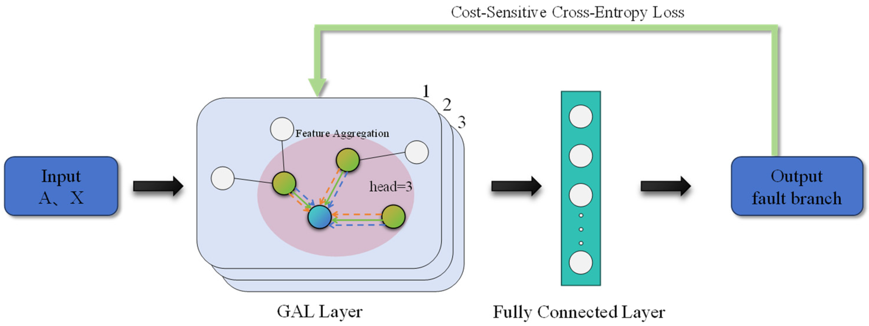
3.4. Fault Location Model

The node feature matrix $X$ is used to store electrical information on each node, and selecting appropriate node features is crucial. Too many node features can complicate data processing, while too few node features can affect the model capability to extract fault features. After a large number of experiments, this study utilized the three-phase voltage current amplitude and zero-sequence voltage current amplitude information as the input feature vector of nodes; namely $X=\left\{V_A,V_B,V_C,V_0,I_A,I_B,I_C,I_0\right\},X\in R^{N\times 8}$, where $N$ is the number of nodes in the distribution network.

Figure 8 shows the structure of the GAT fault classification model. After inputting the adjacency matrix and node feature matrix, the model updates node features through the graph attention layer. To avoid the phenomenon of node over-smooth caused by large information focused on the graph signal, a three-layer GAL is adopted to obtain the spatial distribution characteristics of distribution network fault data. In order to achieve the classification task, the spatial distribution characteristics of the fused distribution network are expanded into one-dimensional vectors and passed through a fully connected layer. Finally, the binary labels of the fault status for each node can be obtained, where “0” indicates a normal state and “1” indicates a fault state.

Here, the GAT consists of three multi-head attention mechanism graph attention layers and one fully connected layer. The first two GALs have three attention heads, and the third GAL has six attention heads.

The pseudo-code for model training based on the proposed method is shown in Algorithm 1 as follows.

Algorithm 1: Pseudo-code for the model. Training process of the CS-GAT

Input:  $\mathrm{training} \mathrm{set} {\mathrm{D}}_{\mathrm{t}\mathrm{r}\mathrm{a}\mathrm{i}\mathrm{n}}\left\{\right(G, X, T\left)\right\}$, batch-size, epochs, learning-rate Output: $\mathrm{predicted} \mathrm{label} Y$

1. Initialize parameters $W_{att}$$, W$ of each GAL and cost-sensitive matrix $\mathrm{C}$

2. Training data normalization and random ordering

3. Splicing of batch training data

4. for epoch to epochs do

5.    $Y\_logits=\mathrm{G}\mathrm{r}\mathrm{a}\mathrm{p}\mathrm{h}\mathrm{A}\mathrm{t}\mathrm{t}\mathrm{e}\mathrm{n}\mathrm{t}\mathrm{i}\mathrm{o}\mathrm{n}\mathrm{N}\mathrm{e}\mathrm{t}\mathrm{w}\mathrm{o}\mathrm{r}\mathrm{k}(G,X,W_{att },W)$

6.    $Y=\mathrm{s}\mathrm{i}\mathrm{g}\mathrm{m}\mathrm{o}\mathrm{i}\mathrm{d}(Y\_logits)$

7.    Calculate the cost-sensitive matrix $C$

8.    Calculate the cost-sensitive loss: $\mathrm{l}\mathrm{o}\mathrm{s}\mathrm{s}={\mathrm{L}\mathrm{o}\mathrm{s}\mathrm{s}}_{\mathrm{C}\mathrm{S}}(Y,T,C)$

9.    Backpropagation to update parameters

10. end for

4. Results and Discussion

4.1. Platform Construction and Data Collection

4.1.1. Construction of Simulation Model

Due to the least obvious fault characteristics when a single-phase grounding fault occurs in a distribution network where the neutral point is not directly grounded, this section focuses on simulating single-phase ground faults occurring at different locations. A standard IEEE-33 bus distribution network model was constructed using the Simulink simulation module. Two photovoltaic-type distributed generators with fixed outputs were connected at nodes 18 and 33, each providing 1 MW of active power and 0 MVar of reactive power. The reference voltage and power of the system were set to 12.66 kV and 20 MW, respectively. A dynamic load model was adopted, with the load sizes at each node fluctuating randomly between 95% and 105% of their reference values.

As shown in Figure 9, ten branches (such as 2, 5, 8, 13, 15, 18, 21, 24, 27, 32) are researched, and simulate the single-phase ground fault occurring in each of the three phases A, B, and C of each branch, respectively, with fault resistance ranging from 50 Ω to 200 Ω. Within 0.2 s after the fault, the voltage and current amplitudes of each node and the zero-sequence voltage and current amplitudes are taken to form the node characteristic data X, with a dimension of (33, 8). Each branch is simulated 100 times for each phase fault situation, totaling 3000 sets of fault characteristic data. While obtaining the feature matrices of each node, the graph structure data G of the distribution network topology and the associated fault labels T are recorded, together forming a single fault data entry. Since the proportion of fault data in reality are small, when constructing the dataset, normal operation and fault conditions are simulated and summarized at a ratio of 9:1. Finally, the dataset is divided into training, validation, and testing sets at a ratio of 8:1:1.

4.1.2. Data Storage and Computation

In neural network training, it is common to use batch-size to process or feed multiple sets of data into the network simultaneously, to improve training efficiency and the model’s generalization capability. Figure 10 illustrates the batch training method in GNN. When multiple sets of data are trained together, the adjacency matrices of individual graphs are concatenated diagonally to form a larger, sparser adjacency matrix. If traditional two-dimensional arrays are still used for storage and computation, this would lead to significant resource waste and performance bottlenecks. Therefore, under the context of handling large-scale graph data, adopting efficient compression storage and computation techniques becomes particularly critical to reduce memory usage and enhance processing speed.

In the specific implementation, the proposed method uses the compressed sparse column format (CSC format) for storing and computing sparse graph structure data. To illustrate the advantages of this approach, the paper provides a complexity analysis of operations on sparse matrices under different storage methods, as shown in

Table 1. Sparse matrix operation complexity.

Operation	Stored in Two-Dimensional Array Format		Stored in CSC Format
	Time Complexity	Space Complexity	Time Complexity	Space Complexity
Matrix-vector multiplication	$O\left(n^2\right)$	$O\left(n\right)$	$\mathrm{O}\left(nnz\right(A\left)\right)$	$O\left(nnz\right(A)+n)$
Matrix-matrix multiplication	$O\left(n^{2}m\right)$	$\mathrm{O}\left(nm\right)$	$O\left(nnz\right(A)\times nnz(B\left)\right)$	$O\left(nnz\right(A\times B\left)\right)$
Matrix transposition	$O\left(n^2\right)$	$O\left(n^2\right)$	$O(nnz\left(A\right)+n)$	$O\left(nnz\right(A)+n)$
Matrix addition	$O\left(n^2\right)$	$O\left(n^2\right)$	$O\left(nnz\right(A)+nnz(B\left)\right)$	$O\left(nnz\right(A+B\left)\right)$

. Here, matrix $A$ has dimensions $n\times n$ and matrix $B$ has dimensions $n\times m$, and $nnz(·)$ denotes the number of non-zero elements in the matrix. Since the compressed sparse column (CSC) format stores only the non-zero elements and their indices of the matrix, there is no need to perform computations or store zero elements. Therefore, it outperforms storage methods based on two-dimensional arrays in terms of both time and space complexity. The efficiency gains and resource savings become more pronounced as the matrix dimensions increase and the matrix becomes sparser.

4.2. Analysis of Model-Related Parameters

4.2.1. Selection of Model Parameters

The parameters used in the model proposed in this paper mainly include the number of GAL layers and the number of attention heads per layer. First, the number of attention heads per GAL layer was set to 3 to analyze the impact of the number of GAL layers on model performance. The specific results are shown in

Table 2. F1-score and time cost of models with different numbers of GALs.

GAL Layers	F1-Score (%)	Time Cost (min)
2	81.49	42
3	98.82	93
4	84.27	158

. From Table 2, it can be observed that the choice of the number of GAL layers has a significant impact on the performance of the fault diagnosis model. When the number of layers is 3, the model achieves the highest F1-score of 98.82%, indicating the best feature extraction effect. When the number of GAL layers is 2 or 4, the F1-score is lower than when the number of layers is 2, suggesting that fewer GAL layers cannot capture complex relationships in the graph, leading to underfitting. On the other hand, too many GAL layers can lead to excessive information propagation, reducing the differences between features in different layers and thus affecting the model’s discriminative power. Additionally, as the number of GAL layers increases, the training time also becomes longer. Therefore, the number of GAL layers in the model proposed in this paper was set to 3. Worth noting is that the normalized time cost is calculated using the shortest training time as the baseline.

After determining the number of GAL layers, an analysis is conducted on the impact of the number of attention heads per layer on model performance. The experimental results are shown in

Table 3. F1-score and time cost of models with different number of heads.

Number of Heads	F1-Score (%)	Time Cost (min)
2	93.42	64
3	97.95	97
4	98.36	131
5	98.62	186
6	98.61	243

. From Table 3, it can be seen that the impact of the number of attention heads on model performance is not monotonous. When the number of attention heads increases from 2 to 3, the model’s performance improves by approximately 4.5%. However, as the number of attention heads continues to increase, the training time significantly increases while the improvement in model performance tends to saturate. Therefore, the selection of the number of attention heads needs to be optimized based on specific application scenarios and datasets. After balancing model performance and training costs, the number of attention heads per layer in the proposed model was set to 3.

Additionally, considering that each GAL layer can extract finer features based on the previous layer, the number of attention heads can be fine-tuned to further improve model performance. In the model proposed in this paper, the first two layers use three attention heads to extract more fundamental features and capture local information for broader feature fusion. In the third layer, the proposed model uses six attention heads to perform more complex integration and reasoning of the extracted features, achieving multi-scale feature fusion and enhancing the model’s ability to learn the representation of input data.

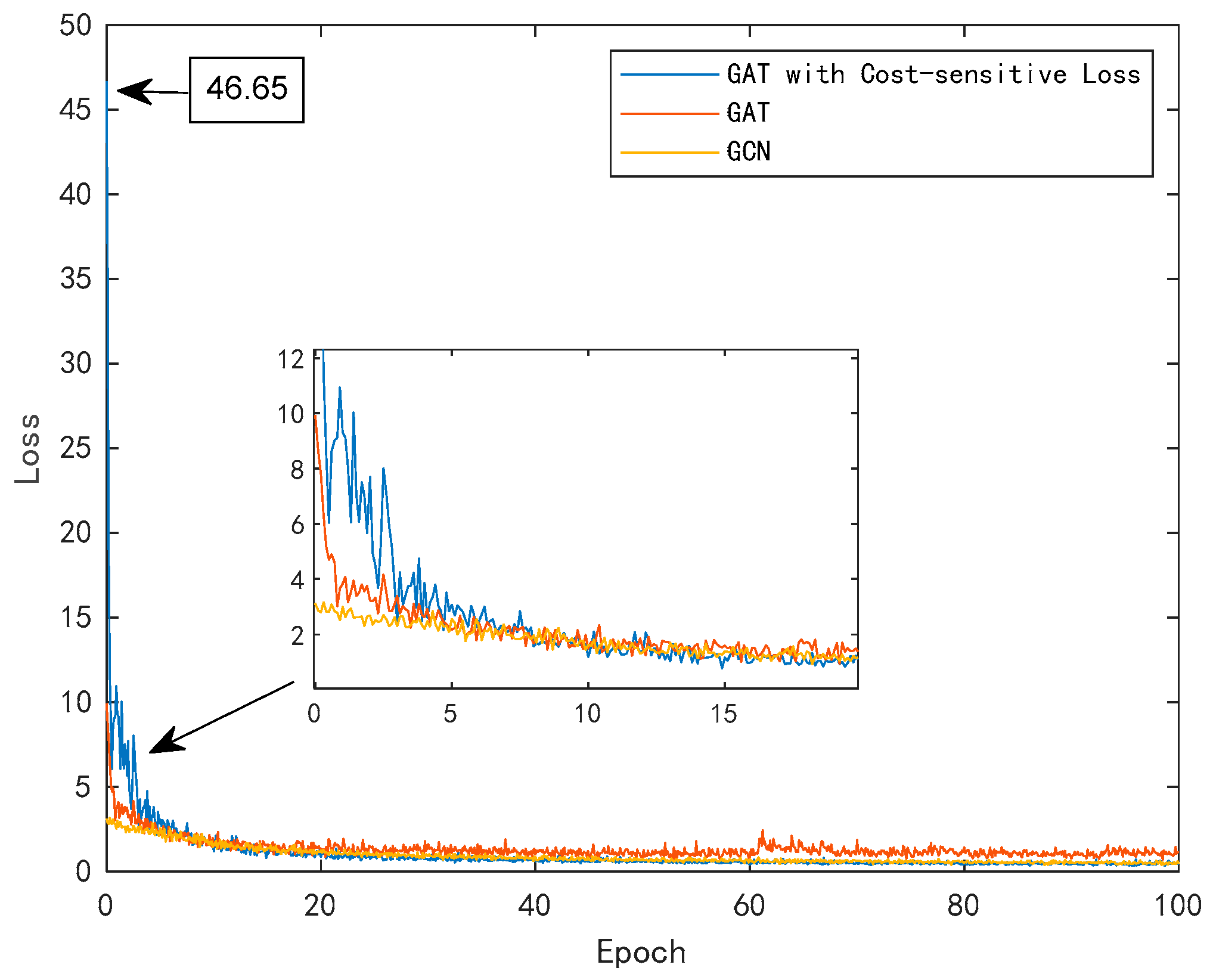
4.2.2. Selection of Training Parameters

During the model training process, the learning rate is set to 0.001, and the number of iterations is set to 100. The ADAM optimizer is used for adaptive adjustment of the learning rate and backpropagation of model parameters, completing the training of the GAT fault localization model by minimizing the cost-sensitive loss. The choice of batch size also affects model performance. Training the model with batch sizes of 32, 64, and 128 yields the results shown in

Table 4. F1-score and time cost under different batch-sizes.

Batch-Size	F1-Score (%)	Time Cost of 100 Epochs (min)
32	98.76	161
64	98.80	99
128	97.61	57

. From Table 4, it can be observed that, under the same number of epochs, the model performance is better when the batch size is 32 or 64 compared to when the batch size is 128. Given that a smaller batch size results in longer training times, the batch size in the proposed model was set to 64.

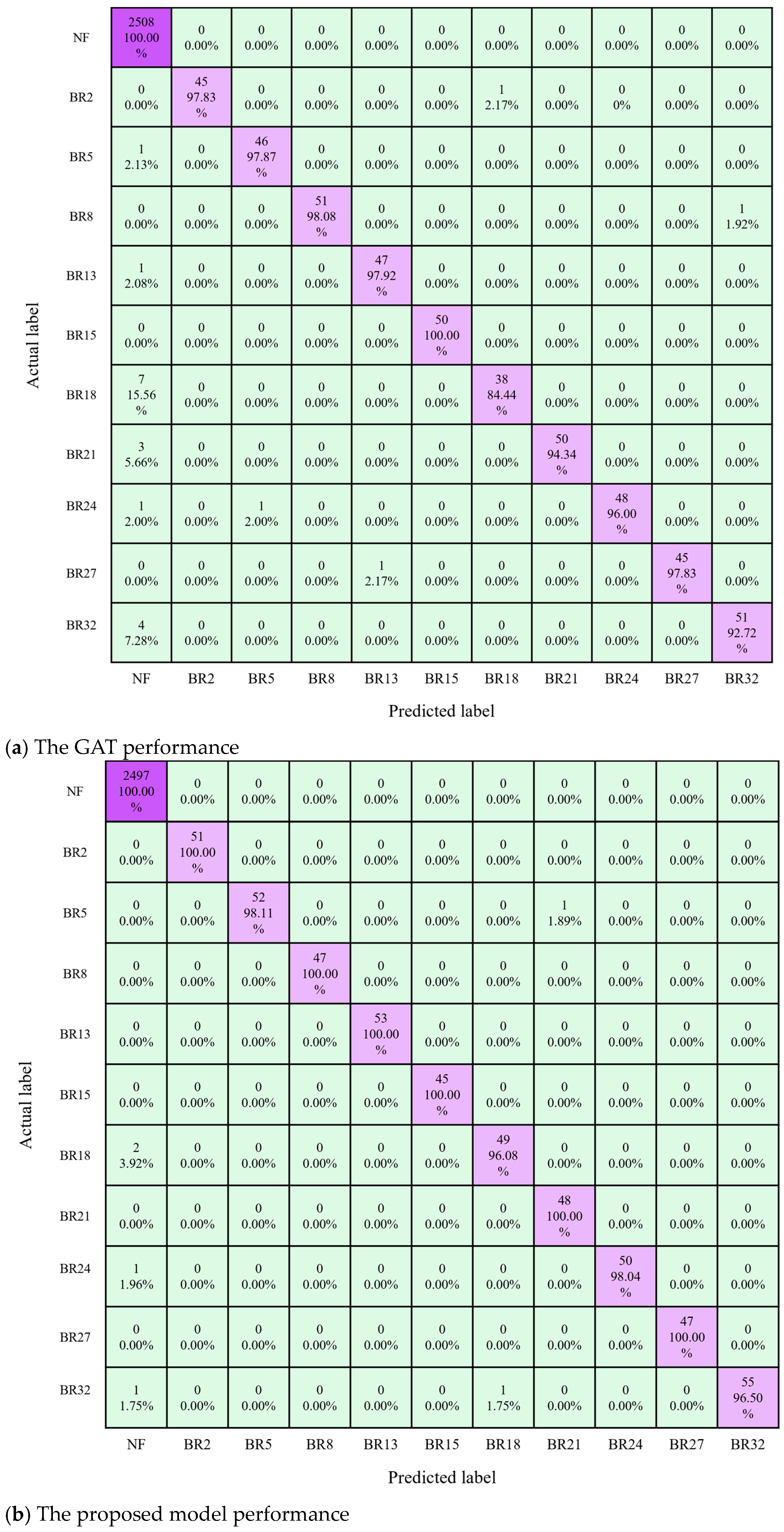
4.3. Fault Location Performance Analysis

Based on the MATLAB 2023a platform, the GCN [27] and GAT [25] based models were reproduced, and a comparative analysis was conducted on the fault localization performance against the proposed method. Figure 11 exhibits the training loss of the proposed method and comprehensively compares GCN and GAT. Due to imbalanced datasets, there are many misclassifications during the initial training phase. However, as the number of training sessions increases, the GAT with cost-sensitive losses learns node features and topological relationships faster, and the loss value decreases rapidly. Traditional GAT is more affected by non-fault data in imbalanced datasets, which leads to lower overall prediction accuracy and is more prone to loss fluctuations and overfitting during training.

To evaluate the performance of the fault localization method proposed in this study, the confusion matrix and F1-score·were introduced for analysis. As shown in Figure 12, each row in the confusion matrix represents the true label of the data sample, and each column represents the predicted label obtained by the model classification. The sum of each row indicates the total number of samples in that class, the elements on the main diagonal indicate the number of samples correctly identified as belonging to that class, and the off-diagonal elements indicate the number of samples incorrectly predicted as belonging to other classes. These data can be used to determine whether the model exhibits confusion between certain classes. When dealing with imbalanced datasets, analyzing the confusion matrix can reveal whether the model overemphasizes or neglects minority classes, thereby providing a better understanding of the model’s actual performance. Figure 12a,b show the test performance of the GAT-based model and the model proposed in this paper, respectively. It can be observed that the model proposed in this paper, which employs a cost-sensitive loss function, enhances the model’s focus on fault samples, resulting in only a few fault branches being misclassified as non-fault branches.

From the confusion matrix shown in Figure 12, it can be seen that both the proposed method and the GAT-based method exhibited ‘false positives’. This is likely due to the higher proportion of non-fault samples in the dataset, leading to an imbalanced dataset. However, the proposed method has a lower false positive rate compared to the GAT-based method. To address the issue of false positives, we can improve the quality of the dataset by collecting more fault samples and applying appropriate preprocessing techniques, thereby training the model more effectively and enhancing the accuracy of fault classification.

The testing results in term of F1-score are shown in

Table 5. F1-score comparison.

Model	F1-Score (%)
proposed	98.97%
GAT	96.09%
GCN	95.40%

. It can be seen from Table 5 that the F1-score value of the model proposed in this study is 98.97%, which is 2.88% higher than the traditional GAT and 3.57% higher than the GCN model. It can be seen that, in the case of imbalanced datasets, the proposed model can focus more on fault feature data, obtaining a high generalization ability.

In practical scenarios, fault sample data for distribution networks are scarcer. To evaluate the model’s performance on small training sets, the training set size was reduced to 90%, 70%, 50%, and 30% of the original amount, and the model was trained accordingly. Testing was then performed using the original test set. The relevant results are detailed in

Table 6. Performance of models under different number of training samples.

Training Set Size (%)	F1-Score (%)
90%	98.23
70%	96.71
50%	91.23
30%	72.76

. It can be observed that the model still performs well even when the dataset is reduced to 50% of its original size. This may be due to the similarity of samples under certain fault conditions, allowing the proposed model to generalize effectively and capture key fault patterns from limited samples.

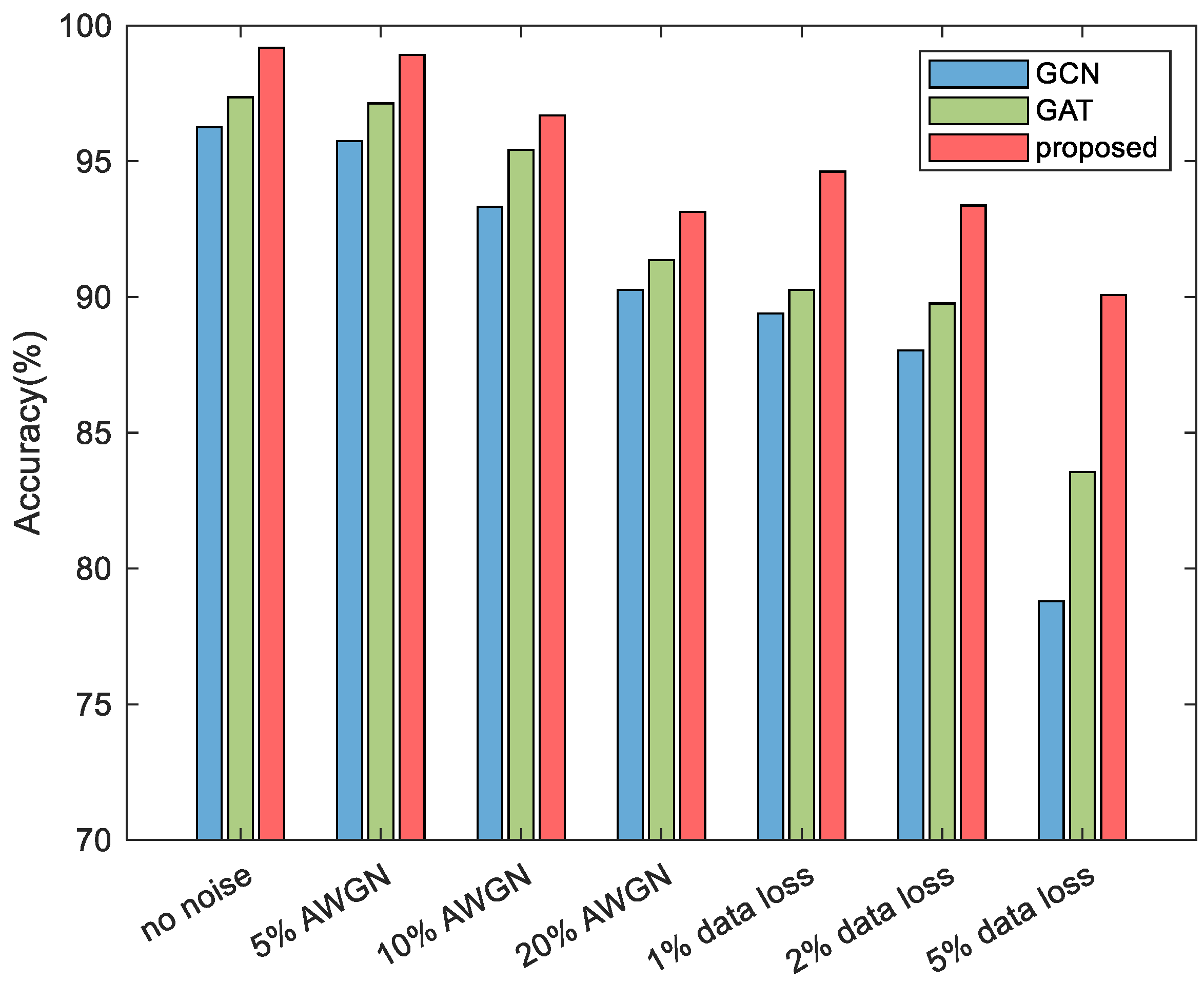
4.4. Impact of Data Disturbance

Considering that actual power measurement data may be subject to data disturbance, this section intends to use the same training dataset to test the anti-interference ability of the GCN, GAT, and the proposed cost-sensitive GAT (CS-GAT) model. Under the premise of a fault resistance of 100 Ω, 200 simulations were conducted for the non-fault condition and the fault condition of 10 branches to construct the equal proportion testing dataset. The stability of the model was verified by adding 60 dB and 30 dB Gaussian white noise to the testing dataset, and two data missing cases with random loss of 1% and 2% feature data. In particular, in the case of missing data, the lost data was filled with 0.

To analyze the impact of data perturbations on model performance, two scenarios were considered: noise interference and data loss. Noise interference was simulated by adding 10%, 15%, 20%, and 25% additive Gaussian white noise to the data. Data loss was simulated by setting 1%, 2%, and 5% of the measurement data to zero. The test results are shown in Figure 13. It can be observed that as the noise increases, the accuracy of all models decreases. However, the proposed model maintains higher localization accuracy compared to the GCN and GAT models, demonstrating strong noise resistance. Compared to noise interference, data loss has a greater impact on model accuracy, but the proposed model still maintains an accuracy above 90%, which is the highest.

4.5. Impact of Fault Resistance on Model Performance

In practical scenarios, fault resistances during short circuits are not limited to specific values, and training samples cannot cover all possible values. Therefore, the model’s ability to locate faults under unknown resistance conditions outside the training samples is also important. This section selects transition resistances within the training range (50–200 Ω) and outside the training range (variations within 50%) to construct a proportionally balanced test dataset, verifying the model’s localization accuracy under different fault transition resistance conditions. The results are shown in Figure 14.

It can be seen that when the resistance value of the fault transition resistor is within the training range, all fault localization methods have high accuracy, but when it exceeds the training range, the fault localization accuracy decreases to varying degrees. Especially when the transition resistance is large, the fault characteristics are weaker and the difference between fault phase and non-fault phase is small, which seriously affects the performance of the fault location model. As shown in Figure 14, the positioning accuracy of the GCN is low, while the proposed model has stronger generalization ability. The proposed model still has a positioning accuracy of 91.32% when the fault resistance is 300 Ω. When the transition resistance is at a small value, due to the more obvious fault characteristics in the case of small resistance, the positioning accuracy of the three models decreases less.

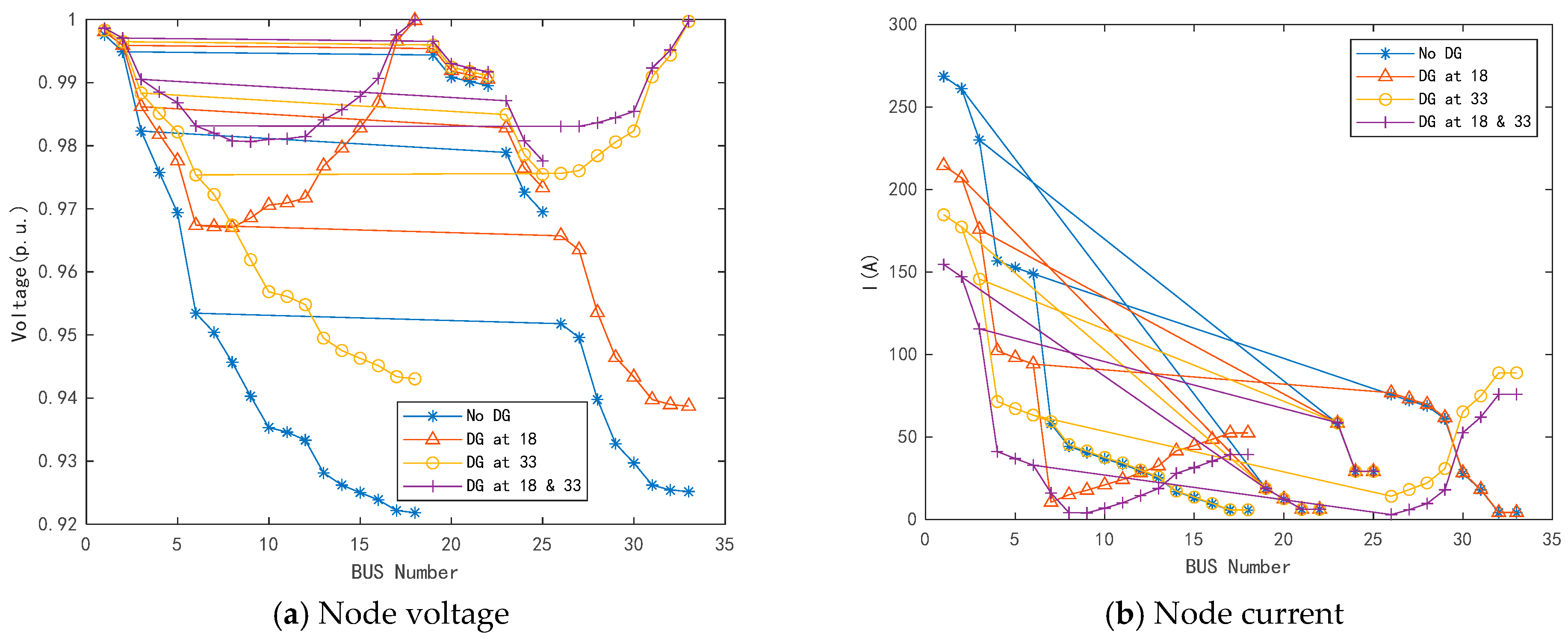
4.6. Impact of DG Access on Model Performance

At present, the penetration rate of DG in distribution networks is about 8% to 12%. With the widespread integration of DG, it is expected that the penetration rate will rapidly increase, potentially exceeding 50% in some areas. To explore the impact of different penetration rates and DG configurations on fault localization performance, this section tests various penetration rates (0%, 5%, 10%, 15%, 30%, 50%) while keeping the load levels at each node constant and the fault resistance at 100 Ω. The testing is divided into two scenarios: one where the DG output is fixed, meaning the output of DG1 and DG2 remains unchanged and equal; and another where the DG output is random, meaning the total output of DGs remains constant but the output of each DG varies randomly. Each scenario involves generating 100 short-circuit fault test cases randomly. Figure 15 shows the impact of the DG penetration rate and output mode on localization accuracy.

It can be observed that as the penetration rate of DGs in the distribution network increases, the fault voltage and current levels rise, making it easier to detect faults in the distribution network. At lower penetration rates, the proposed model demonstrates stable performance. However, when the penetration rate increases to 30% and 50%, the localization accuracy of all models shows a noticeable decline. This may be because the training dataset lacks fault data under high penetration conditions, causing the model to be less sensitive to the characteristics of grid faults under high penetration rates, thereby affecting the fault localization accuracy.

Moreover, the random output of DGs is closer to real-world conditions but can also lead to significant differences in fault characteristics at the same location, placing higher demands on the model’s ability to distinguish between different faults. Under these conditions, the fault localization accuracy of all models is lower than when the DG output is fixed. However, compared to other models, the model proposed in this paper still maintains a localization accuracy above 95%, demonstrating good adaptability to varying distribution network operating states.

5. Conclusions

Accurate and timely fault diagnosis is essential for ensuring the stable operation of distribution networks. This study addresses the limitations of traditional artificial intelligence-based localization methods, which often struggle with adapting to the dynamic topologies of distribution networks due to their reliance on large-scale labeled datasets. To overcome these challenges, a novel fault location method utilizing a cost-sensitive GAT model is proposed. By integrating the physical structure of the distribution network as a critical component of the model training process, the model’s ability to perceive and interpret relevant information is enhanced. Specifically, the mapping of electrical nodes and lines to vertices and edges within the GAT framework, coupled with attention weights derived from the correlation of adjacent node fault characteristics, improves the model’s adaptability to topological changes. Furthermore, the implementation of a cost-sensitive matrix helps to balance class distributions, thereby enhancing the robustness and generalization capability of the model.

Experimental validation was conducted on the IEEE-33 bus distribution system, incorporating factors such as data disturbances, distributed power supply access, and topology changes to assess the model’s anti-interference performance. The results demonstrate that the proposed fault location method achieves high positioning accuracy and excellent robustness, even under varying conditions.

The study provides a robust and adaptable solution for fault localization in distribution networks, contributing to improved reliability and stability in smart grid operations. Future work will focus on further validating the model in diverse real-world scenarios and exploring the integration of additional contextual information to enhance performance.

References

1. Gurajapathy, S.S.; Mokhlis, H.; Illias, H.A. Fault location and detection techniques in power distribution systems with distributed generation: A review. Renew. Sustain. Energy Rev. 2017, 74, 949–958. [Google Scholar] [CrossRef]
2. Xu, J.; Wu, Z.; Yu, X.; Hu, Q.; Zhu, C.; Dou, X.; Gu, W.; Wu, Z. A new method for optimal FTU placement in distribution network under consideration of power service reliability. Sci. China Technol. Sci. 2017, 60, 1885–1896. [Google Scholar] [CrossRef]
3. Dashti, R.; Ghasemi, M.; Daisy, M. Fault location in power distribution network with presence of distributed generation resources using impedance based method and applying π line model. Energy 2018, 159, 344–360. [Google Scholar] [CrossRef]
4. Vieira, F.L.; Filho, J.M.C.; Silveira, P.M.; Guerrero, C.A.V.; Leite, M.P. High impedance fault detection and location in distribution networks using smart meters. In Proceedings of the 18th International Conference on Harmonics and Quality of Power (ICHQP), Ljubljana, Slovenia, 13–16 May 2018; pp. 1–6. [Google Scholar]
5. Yuan, Y.; Low, S.H.; Ardakanian, O.; Tomlin, C.J. Inverse Power Flow Problem. IEEE Trans. Control Netw. Syst. 2023, 10, 261–273. [Google Scholar] [CrossRef]
6. Yue, Y.; Zhao, H.; Zhao, Y.; Wang, H. A study of distribution network fault location including Distributed Generator based on improved genetic algorithm. In Proceedings of the 3rd International Conference on System Science, Engineering Design and Manufacturing Informatization, Chengdu, China, 20–21 October 2012; pp. 103–106. [Google Scholar]
7. Jiang, K.; Tong, X. Fault section location method based on fuzzy self-correction bat algorithm in non-solidly earthed distribution network. In Proceedings of the 2017 2nd International Conference on Power and Renewable Energy (ICPRE), Chengdu, China, 20–23 September 2017; pp. 485–489. [Google Scholar]
8. Meng, F.; Zhao, S.; Li, Z.; Li, S. Distribution Network Fault Location Based on Improved Binary Particle Swarm Optimization. In Proceedings of the 2018 Chinese Intelligent Systems Conference, Wenzhou, China, 13–14 December 2018; Lecture Notes in Electrical Engineering. Springer: Singapore, 2018; Volume 528, pp. 181–189. [Google Scholar]
9. Tao, C.; Wang, J.; Wang, T.; Yang, Y. An improved spiking neural P systems with anti-spikes for fault location of distribution networks with distributed generation. In Proceedings of the Bio-inspired Computing: Theories and Applications (BIC-TA 2017) Communications in Computer and Information Science, Harbin, China, 1–3 December 2017; Springer: Singapore, 2017; Volume 791, pp. 380–395. [Google Scholar]
10. Sapountzoglou, N.; Lago, J.; Raison, B. Fault diagnosis in low voltage smart distribution grids using gradient boosting trees. Electr. Power Syst. Res. 2020, 182, 106254. [Google Scholar] [CrossRef]
11. Zhao, J.; Ma, N.; Hou, H.; Zhang, J.; Ma, Y.; Shi, W. A fault section location method for small current grounding system based on HHT. In Proceedings of the China International Conference on Electricity Distribution (CICED), Tianjin, China, 17–19 September 2018; pp. 1769–1773. [Google Scholar]
12. Liang, R. Fault location method in power network by applying accurate information of arrival time differences of modal traveling waves. IEEE Trans. Ind. Inform. 2020, 16, 3124–3132. [Google Scholar] [CrossRef]
13. Naidu, O.D.; Pradhan, A.K. Precise traveling wave-based transmission line fault location method using single-ended data. IEEE Trans. Ind. Inform. 2021, 17, 5197–5207. [Google Scholar] [CrossRef]
14. Shafiullah, M.; Abido, M.A.; Abdel-Fattah, T. Distribution grids fault location employing ST based optimized machine learning approach. Energies 2018, 11, 2328. [Google Scholar] [CrossRef]
15. Moloi, K.; Yusuff, A.A. A Support Vector Machine Based Fault Diagnostic Technique in Power Distribution Networks. In Proceedings of the 2019 Southern African Universities Power Engineering Conference/Robotics and Mechatronics/Pattern Recognition Association of South Africa (SAUPEC/RobMech/PRASA), Bloemfontein, South Africa, 28–30 January 2019; pp. 229–234. [Google Scholar]
16. Swetapadma, A.; Yadav, A. A novel single-ended fault location scheme for parallel transmission lines using k-nearest neighbor algorithm. Comput. Electr. Eng. 2018, 69, 41–53. [Google Scholar] [CrossRef]
17. Ru, J.; Luo, G.; Shang, B.; Luo, S.; Liu, W.; Wang, S. Fault Line Selection and Location of Distribution Network Based on Improved Random Forest Method. In Proceedings of the 2022 4th International Conference on Smart Power & Internet Energy Systems (SPIES), Beijing, China, 27–30 October 2022; pp. 1179–1184. [Google Scholar]
18. Rafinia, A.; Moshtagh, J. A new approach to fault location in three-phase underground distribution system using combination of wavelet analysis with ANN and FLS. Int. J. Electr. Power Energy Syst. 2014, 55, 261–274. [Google Scholar] [CrossRef]
19. Mirshekali, H.; Dashti, R.; Keshavarz, A.; Shaker, H.R. Machine learning-based fault location for smart distribution networks equipped with micro-PMU. Sensors 2022, 22, 945. [Google Scholar] [CrossRef] [PubMed]
20. Shadi, M.R.; Ameli, M.T.; Azad, S. A real-time hierarchical framework for fault detection, classification, and location in power systems using PMUs data and deep learning. Int. J. Electr. Power Energy Syst. 2022, 134, 107399. [Google Scholar] [CrossRef]
21. Liao, W.; Bak-Jensen, B.; Pillai, J.R.; Wang, Y.; Wang, Y. A review of graph neural networks and their applications in power systems. J. Mod. Power Syst. Clean Energy 2022, 10, 345–360. [Google Scholar] [CrossRef]
22. Hu, J.; Hu, W.; Chen, J.; Cao, D.; Zhang, Z.; Liu, Z.; Chen, Z.; Blaabjerg, F. Fault Location and Classification for Distribution Systems Based on Deep Graph Learning Methods. J. Mod. Power Syst. Clean Energy 2023, 11, 35–51. [Google Scholar] [CrossRef]
23. Chanda, D.; Soltani, N.Y. Graph-Based Multi-Task Learning for Fault Detection in Smart Grid. In Proceedings of the 2023 IEEE 33rd International Workshop on Machine Learning for Signal Processing (MLSP), Rome, Italy, 17–20 September 2023; pp. 1–6. [Google Scholar]
24. Chen, K.; Hu, J.; Zhang, Y.; Yu, Z.; He, J. Fault location in power distribution systems via deep graph convolutional networks. IEEE J. Sel. Areas Commun. 2020, 38, 119–131. [Google Scholar] [CrossRef]
25. Veličković, P.; Cucurull, G.; Casanova, A.; Romero, A.; Lio, P.; Bengio, Y. Graph attention networks. arXiv 2017, arXiv:1710.10903. [Google Scholar]
26. Kashem, M.A.; Ganapathy, V.; Jasmon, G.B.; Buhari, M.I. A novel method for loss minimization in distribution networks. In Proceedings of the DRPT2000. International Conference on Electric Utility Deregulation and Restructuring and Power Technologies. Proceedings (Cat. No. 00EX382), London, UK, 4–7 April 2000; IEEE: Piscataway, NJ, USA, 2000; pp. 251–256. [Google Scholar]
27. Kipf, T.N.; Welling, M. Semi-supervised classification with graph convolutional networks. arXiv 2016, arXiv:1609.02907. [Google Scholar]
Figure 1. Graph structure of IEEE-33 bus distribution system.
Processes 12 02312 g001
Figure 2. Influence of DG access on node voltage and node current.
Processes 12 02312 g002
Figure 3. Power flow of distribution network with DGs.
Processes 12 02312 g003
Figure 4. Structure of proposed fault location framework.
Processes 12 02312 g004
Figure 5. Graph attention layer.
Processes 12 02312 g005
Figure 6. Multi-head graph attention mechanism ( M = 3 ).
Processes 12 02312 g006
Figure 7. The process of transforming graph relationships into adjacency matrices.
Processes 12 02312 g007
Figure 8. Model structure.
Processes 12 02312 g008
Figure 9. Fault location selection in IEEE-33 bus distribution network.
Processes 12 02312 g009
Figure 10. Batch training of n-group graph data.
Processes 12 02312 g010
Figure 11. Training loss of different fault location models.
Processes 12 02312 g011
Figure 12. Testing confusion matrix of the GAT and proposed model.
Processes 12 02312 g012
Figure 13. Impact of data disturbances on model performance.
Processes 12 02312 g013
Figure 14. Impact of fault resistance on model performance.
Processes 12 02312 g014
Figure 15. Comparison of the effects of DG integration on the model.
Processes 12 02312 g015