Optimisation of Ammonia Production and Supply Chain from Sugarcane Ethanol and Biomethane: A Robust Mixed-Integer Linear Programming Approach

Abstract

Low-carbon ammonia production is crucial for sustainable development. Brazil, a top ethanol producer, can boost competitiveness and cut emissions by integrating ammonia and ethanol production. However, optimal location and production strategy identification is challenging due to existing possibilities and uncertainties. For that, a new MILP superstructure with robust optimisation was developed and used to analyse low-carbon ammonia production integration in the ethanol industry in São Paulo state by ethanol and biomethane routes, in two different scenarios. As for the results, in scenario 1, biomethane and ethanol investments were USD 3.846 M and USD 314 M. In scenario 2, the investments were USD 316 M for biomethane and USD 259 M for ethanol. Despite the higher investment, the biomethane route results in lower hydrogen production cost (USD 1880/tonne) due to raw material prices; however, ethanol displays a higher hydrogen potential, consuming just 8% of total production against 54% of vinasse availability, which is used for biodigestion and biomethane production. In conclusion, the results suggest that the northern region of São Paulo has greater potential for ammonia facilities due to resource availability. These findings can inform and support more comprehensive studies and public incentive policies.

1. Introduction

Ammonia production is of great significance to global agriculture, as it constitutes a principal component of nitrogen fertilizers. In Brazil, the significance of ammonia is further amplified by the country’s status as one of the largest agricultural producers globally [1]. This sector constitutes a pivotal component of the Brazilian economy, contributing a considerable proportion of the country’s Gross Domestic Product and imports. It is therefore of paramount importance to ensure the sustainable and efficient production of ammonia if agricultural productivity and, consequently, the Brazilian economy are to be maintained.

Ammonia is produced on an industrial scale by the Haber–Bosch (HB) process, which involves the reaction between nitrogen (N₂) and hydrogen (H₂). It is estimated that ammonia production accounts for approximately 2% of global energy consumption [2] and is responsible for approximately 1% of greenhouse gas (GHG) emissions, making it an industrial activity with a considerable environmental impact [3]. A significant proportion of the emissions associated with the Haber–Bosch process is attributable to the production of its raw materials, with hydrogen representing a significant contributor. This hydrogen is frequently derived from fossil resources, including natural gas and coal. Consequently, the decarbonisation of ammonia production is of paramount importance if the global climate is to be stabilised, the targets set out in international carbon reduction agreements are to be met and a low-carbon economy is to be developed. In order to reduce the emissions associated with hydrogen production, a number of approaches are being explored, including biomass gasification [2,4] and the use of renewable energy [5,6]. Cameli et al. [7] put forth a proposed plant design for the sustainable production of ammonia. This design employs water electrolysis and cryogenic distillation to generate hydrogen and nitrogen, respectively. The authors posit that the utilisation of wind energy results in a 92% reduction in carbon emissions in comparison to the process based on methane steam reforming, with a corresponding reduction in CO₂ emissions of 0.36 kgCO₂·kgNH₃⁻¹. Nevertheless, the high cost of the electrolyser and electricity represent the primary obstacles to economic viability. Nevertheless, the authors conclude that production can be competitive with traditional methods in small-scale stand-alone applications, particularly in the context of carbon taxes and the advancement of electrolyser technology. The same conclusions are presented by Osman et al. [5] and Fúnez Guerra et al. [6]. Osman et al. [5] evaluated the potential for green ammonia production in high insolation regions, including seawater desalination, water electrolysis, air distillation and the Haber–Bosch process. The feasibility of a green ammonia production plant in Chile was explored, utilising renewable energies (solar, wind and hydraulic), with a minimum selling price of 400 EUR/tNH₃. Fúnez Guerra et al. [6] demonstrated that the production of green ammonia and its transport to Japan could be a potentially profitable venture, with a relatively short payback period. However, this profitability is mainly contingent upon the price of electricity and the cost of the electrolyser, with maximum values of 26 EUR/MWh and 800 EUR/kW, respectively. Flórez-Orrego et al. [2] compared the use of biomass gasification to partially or totally replace methane in an integrated syngas and ammonia production plant. The authors demonstrated that by completely replacing natural gas with synthesis gas from biomass gasification, the total CO₂ emission was −2.276 tCO₂·tNH₃⁻¹, indicating the benefits of producing ammonia from biomass. Samini et al. [4] conducted a study investigating the energy and exergetic efficiency of the gasification of various biomasses using different gasification agents, including air, steam and air/steam. The authors concluded that the steam gasification of pine wood resulted in the highest exergy efficiency. Additionally, the results demonstrated that a higher steam/biomass ratio and temperature, in conjunction with a lower moisture content, led to higher energy efficiency values.

Brazil is one of the world’s most significant producers and exporters of agricultural products, consequently occupying a prominent position in the global fertilizer consumption market. Nevertheless, approximately 80% of the national fertilizer market is supplied by imported products, which has led to the issue of increasing the production capacity of this resource becoming a strategic one [8]. Given the considerable consumption of natural gas for hydrogen production, the defossilisation of ammonia production is a crucial step in Brazil’s pursuit of sustainable development. The sugarcane sector is of great economic importance to Brazil, ranking as one of the world’s leading producers of sugarcane and ethanol. The production of ethanol from sugarcane results in the generation of an effluent known as vinasse. For every litre of ethanol produced, approximately 12 L of this effluent is obtained. Due to its high organic matter content, the biodigestion of vinasse has received considerable attention and is the subject of numerous studies. It is estimated that the state of São Paulo has the potential to produce 3.63 billion Nm³ of biogas [9], which could be used as a substitute of natural gas for hydrogen production. Another alternative for hydrogen production is ethanol, whose conversion can be carried out by a process called steam reforming. The well-established production technology and well-developed storage and distribution systems make ethanol a feedstock with high potential for hydrogen production [10,11,12].

For a low-carbon economy to be viable, it is necessary to overcome a number of barriers, including the location and availability of sustainable raw materials, as well as transportation costs. Furthermore, uncertainties regarding the supply, transportation, demand and price of resources make it challenging to identify the most appropriate production strategy. Consequently, supply chain optimisation is essential to overcome these challenges [13]. The utilisation of superstructure-based methodologies is a prevalent approach in the engineering of logistics networks, encompassing the transportation, processing and distribution of biomass and biofuels. Illustrative studies include the work of Abdul Razik and colleagues [14], who employed a linear-programming-based methodology to optimise the operational planning of a biomass supply chain. In a similar vein, Jonker et al. [15] devised a model based on linear programming to ascertain the optimal location of first-generation ethanol production plants derived from sugar cane and second-generation ethanol production plants derived from eucalyptus. This was conducted by considering production costs, greenhouse gas (GHG) emissions and the projected expansion of biomass supply areas by 2030. Considering the availability of raw materials, production technologies, transport options and the location of supply stations, Li et al. [16] presented a mathematical model for designing hydrogen supply networks, with a particular focus on the transport sector. The model was then applied to a case study in a region of France, the results of which demonstrate the importance of considering price, demand and carbon offsets within an integrated framework when making decisions about the design of a hydrogen supply network.

Despite the different formulations found, they do not consider the uncertainty present in essential parameters for economic viability, such as the purchase and sale prices of resources. The issue of parameter uncertainty within mathematical programming is widely recognised as one of the main challenges in optimisation and can be addressed using stochastic methods or robust optimisation [17]. Stochastic methods assume that uncertainty can be expressed in the form of probability functions and therefore require a large amount of data, which makes them difficult to apply when this information is not available. To deal with cases where the amount of information is insufficient, robust optimisation is a promising alternative and has been applied in several studies [18,19,20,21,22]. Based on the above, this work aims to present a superstructure based on mixed-integer linear programming with robust optimisation for evaluating the decarbonisation of ammonia production by integrating ammonia and ethanol production in the state of São Paulo, Brazil. Two routes, biomethane and ethanol, were evaluated in two different scenarios, considering a new facility construction, with undetermined location, and the use of existing infrastructure to provide the resources required for an ammonia process at a defined location. Despite the cited studies, no other research was identified that had employed the proposed methodology in this context. Consequently, in addition to introducing an innovative methodology, the findings of this study can inform more comprehensive investigations and contribute to the formulation of public policies designed to facilitate the integration of these sectors. This is due to the insights gained from the existing considerations and the information incorporated into the analyses. Although this work applies the model in a specific context, low-carbon ammonia production in the state of São Paulo, the presented formulation was constructed in a generic way, allowing it to be applied in different contexts, scenarios and areas.

2. Superstructure Formulation

The formulation presented in this paper is an extension and adaptation of the work by Garcia and Ensinas [23], whose MILP formulation considers the selection of processes with scale adjustment, so that a biorefinery can meet the demand for a product, given the availability of a set of resources, and the possibility of the different processes exchanging heat with each other. However, the formulation described considers that every resource consumed or sold has been bought or produced locally, so it does not interact with other locations. In addition, the uncertainty that exists in purchase and sale prices is not considered in the objective function. Therefore, in order to take into account the constraints described above, the mass balance restrictions and the objective function were adjusted, as will be shown in this section, as well as the entire formulation used. As in the work by Garcia and Ensinas [23], to represent each of the processes considered, physical models based on the mass and energy balance of the technology were inserted into the superstructure, each of which was built on the basis of previously published articles describing the main flows of consumption and production of resources, such as vinasse and biomethane, as well as the associated investment costs. The adjusted constraints followed the MILP formulation and were implemented in the LINGO v.21 software [24]. Figure 1 shows a representation of the superstructure workflow.

2.1. Main Sets’ Definition

The formulation is organised into different sets, subsets and their combinations, allowing the inclusion and exclusion of processes and their parameters in a more efficient and structured manner. There are four main sets: RESOURCE (R), UNIT (U), PLACE (P) and MODAL (M). Every resource, element r (r ∈ R), represents any entity that can be transported, such as biomass. Every unit, element u (u ∈ U), represents a given process that consumes a resource and produces another one. Each element u is inserted into the superstructure as a physical model, together with the input flows of the resources it consumes (IARu,r) and produces (OARu,r). The elements of the PLACE set (p ∈ P) represent the different locations that are considered, while the elements of the MODAL set (m ∈ M) represent the different modes of transport that are considered.

2.2. Unit Selection and Scale Adjustment

The selection and scale adjustment of a unit at a place is performed by Equation (1), where ${\mathrm{CapMin}}_{\mathrm{u}}$ and ${\mathrm{CapMax}}_{\mathrm{u}}$ are the maximum and minimum limits for scale adjustment that a unit can have, ${\mathrm{y}}_{\mathrm{u},\mathrm{p}}$ is a binary variable that represents the existence of that unit in that place and ${\mathrm{w}}_{\mathrm{u},\mathrm{p}}$ is a continuous variable responsible for the scaling of that unit and its flows at a specific place, increasing when w_u,p > 1, or decreasing when w_u,p < 1. When selected for that place, a unit has its ${\mathrm{y}}_{\mathrm{u},\mathrm{p}}$ equal to one, and its ${\mathrm{w}}_{\mathrm{u},\mathrm{p}}$ is limited by ${\mathrm{C}\mathrm{a}\mathrm{p}\mathrm{M}\mathrm{i}\mathrm{n}}_{\mathrm{u}}$ and ${\mathrm{C}\mathrm{a}\mathrm{p}\mathrm{M}\mathrm{a}\mathrm{x}}_{\mathrm{u}}$. If not selected, ${\mathrm{y}}_{\mathrm{u}}$ assumes a value of zero, resulting in a ${\mathrm{w}}_{\mathrm{u}}$ equal to zero.

$${\mathrm{CapMin}}_{\mathrm{u}}{\mathrm{y}}_{\mathrm{u},\mathrm{p}}\le {\mathrm{w}}_{\mathrm{u},\mathrm{p}}\le {\mathrm{CapMax}}_{\mathrm{u}}{\mathrm{y}}_{\mathrm{u},\mathrm{p}}\hspace{1em}\hspace{1em}\hspace{1em}\forall u\in \mathrm{U},\forall \mathrm{p}\in \mathrm{P},$$

(1)

2.3. Mass Balance

Similarly to the approach proposed by Garcia and Ensinas [23], the methodology utilises the concept of scaling, whereby each unit u, representing a specific process, is represented by a physical model. This comprises an input flow IAR_u,r and an output OAR_u,r for each resource r. In the case under consideration, the scale of a unit can be expanded or reduced. To this end, a scaling variable (w_u,p) was employed for each unit in each location, which multiplies each of the input/output flows. This allows the consumption (cons_u,r,p) and production (prod_u,r,p) of resources of that unit in that location to be calculated, as presented in Equations (2) and (3).

$${\mathrm{OAR}}_{\mathrm{u},\mathrm{r}}{\mathrm{w}}_{\mathrm{u},\mathrm{p}}-{\mathrm{prod}}_{\mathrm{u},\mathrm{r},\mathrm{p}}=0\hspace{1em}\hspace{1em}\hspace{1em} \forall \mathrm{u}\in \mathrm{U}, \forall \mathrm{r}\in \mathrm{R}, \forall \mathrm{p}\in \mathrm{P}$$

(2)

$${\mathrm{IAR}}_{\mathrm{u},\mathrm{r}}{\mathrm{w}}_{\mathrm{u},\mathrm{p}}-{\mathrm{cons}}_{\mathrm{u},\mathrm{r},\mathrm{p}}=0\hspace{1em}\hspace{1em}\hspace{1em}\forall \mathrm{u}\in \mathrm{U}, \forall \mathrm{r}\in \mathrm{R}, \forall \mathrm{p}\in \mathrm{P}$$

(3)

The mass balance, presented in Equation (4), is applied to each resource (r) and location (p). The superstructure assumes that any resource produced or purchased in a location must be consumed or sold, either at the location of production or at another location. In order to consider these possibilities, the mass balance is composed of six flows: consumption (cons_u,r,p), production (prod_u,r,p), purchase (bought_r,p), sale (sold_r,p), input by transport from the transfer of resources from one location (p^′) to another (p) (transfIn_r,p^′,p) and the output of resources by transport from one location to another (transfOut_r,p,p^′), with these both being dependent on the number of hours that the processes operate, which is represented by fop.

$$\begin{array}{c}{\mathrm{bought}}_{\mathrm{r},\mathrm{p}}+{\displaystyle \sum _{\mathrm{u}}}{\mathrm{prod}}_{\mathrm{u},\mathrm{r},\mathrm{p}}\mathrm{fop}+{\displaystyle \sum _{p^{\prime }}}{transfIn}_{\mathrm{r},{\mathrm{p}}^{\prime },\mathrm{p}}=\\ {\displaystyle \sum _{\mathrm{u}}}{\mathrm{cons}}_{\mathrm{u},\mathrm{r},\mathrm{p}}\mathrm{fop}+{\mathrm{sold}}_{\mathrm{r},\mathrm{p}}+{\displaystyle \sum _{p^{\prime }}}{transfOut}_{\mathrm{r},\mathrm{p},{\mathrm{p}}^{\prime }}\hspace{1em}\hspace{1em}\hspace{1em}\forall \mathrm{r} \in \mathrm{R}, \forall \mathrm{p} \in \mathrm{P}\end{array}$$

(4)

2.4. Transport Constraints

The equations in question (5, 6 and 7) are responsible for the transportation of resources between the locations included in the problem formulation. Equation (5) states that the mass of every resource that enters and is transported to location p is given by the sum of the masses of that resource transported by the different modes considered. Equation (6) states that the mass of every resource that leaves and is transported from location p towards location p^′ is given by the sum of that resource transported by the different modes considered. Equation (7) states that the mass of resource r that leaves p^′ for p by mode mo is equal to the mass that entered p by mode mo, thus ensuring that there is no loss due to transport.

$${transfIn}_{\mathrm{r},{\mathrm{p}}^{\prime },\mathrm{p}}=\sum _{mo}{transfInModal}_{\mathrm{r},{\mathrm{p}}^{\prime },\mathrm{p},\mathrm{mo}} \forall \mathrm{r} \in \mathrm{R}, \forall \mathrm{p},{\mathrm{p}}^{\prime } \in \mathrm{P}, \forall \mathrm{mo} \in \mathrm{Mo}$$

(5)

$${transfOut}_{\mathrm{p},{\mathrm{p}}^{\prime },\mathrm{r}}=\sum _{mo}{transfOutModal}_{\mathrm{p},{\mathrm{p}}^{\prime },\mathrm{r},\mathrm{mo}} \forall \mathrm{r} \in \mathrm{R}, \forall \mathrm{p},{\mathrm{p}}^{\prime } \in \mathrm{P}, \forall \mathrm{mo} \in \mathrm{Mo}$$

(6)

$${transfOutModal}_{{\mathrm{p}}^{\prime },\mathrm{p},\mathrm{r},\mathrm{mo}} ={transfInModal}_{{\mathrm{p}}^{\prime },\mathrm{p},\mathrm{r},\mathrm{mo}} \forall \mathrm{r} \in \mathrm{R}, \forall \mathrm{p},{\mathrm{p}}^{\prime } \in \mathrm{P}, \forall \mathrm{mo} \in \mathrm{Mo}$$

(7)

2.5. Availability and Demand Constraints

Equations (8) and (9) are the availability and demand constraints, respectively. Equation (8) ensures that every resource r bought is available at that place p, and Equation (9) ensures that every resource r sold to the place p is demanded at the place p.

$${\mathrm{bought}}_{\mathrm{r},\mathrm{p}} \le {\mathrm{avail}}_{\mathrm{r},\mathrm{p}}\hspace{1em}\hspace{1em}\hspace{1em}\forall \mathrm{r} \in \mathrm{R}$$

(8)

$${\mathrm{sold}}_{\mathrm{r},\mathrm{p}} \le {\mathrm{demand}}_{\mathrm{r},\mathrm{p}}\hspace{1em}\hspace{1em}\hspace{1em}\forall \mathrm{r} \in \mathrm{R}$$

(9)

2.6. Unit Capital Cost and Investment Cost Linearisation

Every unit placed in the superstructure has a reference scale, as previously stated and carried out by Garcia and Ensinas [23]. Each unit also has a capital investment cost to the referenced scale that has to be adjusted, in addition to the resource consumption and output for each unit. In order to preserve the model’s linearity, a piecewise linearisation of the capital cost function was carried out for each process because capital costs in processes may change nonlinearly. In order to carry out this linearisation, the cost curve was obtained as a function of the scaling factor (w_u,p) using Equation (10) where se is a scaling exponent, C_u,p is the adjusted capital cost for unit u at location p and the annualised capital cost at the reference scale is represented by C0_u. As seen in Figure 2, the curve is then divided into three levels, each of which has a minimum and maximum value, designated as CapMin_u,l and CapMax_u,l accordingly. The Supplementary Materials (Table S1) include the linearised capital cost curve for each process taken into consideration in this work.

$${\mathrm{C}}_{\mathrm{u},\mathrm{p}}={ \mathrm{C}0}_{\mathrm{u}}{\mathrm{w}}_{\mathrm{u},\mathrm{p}}^{\mathrm{se}}$$

(10)

One of the fractured ranges must be chosen at the same time as a unit. Equation (1) is then rewritten as Equation (11). Only one level is chosen per unit at each location thanks to Equation (12). The binary variable (y_u,l,p) takes on the value 0 if no level is chosen. The equality of w_u,p with respect to w_u,l,p of the chosen level is guaranteed by Equation (13).

$${\mathrm{CapMin}}_{\mathrm{u},\mathrm{l}}{\mathrm{y}}_{\mathrm{u},\mathrm{l}} \le {\mathrm{wl}}_{\mathrm{u},\mathrm{l}} \le {\mathrm{CapMax}}_{\mathrm{u},\mathrm{l}}{\mathrm{y}}_{\mathrm{u},\mathrm{l}}$$

(11)

$$\sum _{\mathrm{l}}{\mathrm{yl}}_{\mathrm{u},\mathrm{l}} \le 1$$

(12)

$$\sum _{\mathrm{l}}{\mathrm{wl}}_{\mathrm{u},\mathrm{l}}={\mathrm{w}}_{\mathrm{u}}$$

(13)

In order to calculate the unit investment cost, Equation (14) was employed, where a_u,l and b_u,l represent the angular and linear coefficients of each linearised interval, respectively. The maintenance and operation costs (MC, OC), annualisation factor (AF) and other costs (LC) were fixed at 0.06, 0.086, 0.086 and 0.1, respectively. The following Equations (15)–(17) are employed to calculate the resource acquisition cost, product commercialisation revenue and carbon credit revenue, respectively. The variables ResCost_r, MP_r, PC_r and CarbVal represent the cost of resource r, the market price of resource r, the commercialisation revenue of resource r and the carbon credit price, respectively.

$${\mathrm{UCC}}_{\mathrm{u}}=\sum _{\mathrm{l}}({\mathrm{a}}_{\mathrm{u},\mathrm{l}}{\mathrm{wl}}_{\mathrm{u},\mathrm{l}}+{\mathrm{b}}_{\mathrm{u},\mathrm{l}}{\mathrm{y}}_{\mathrm{u},\mathrm{l}})·\mathrm{AF}·(1+\mathrm{MC}+\mathrm{OC}+\mathrm{LC})$$

(14)

$${\mathrm{RC}}_{\mathrm{r}}={\mathrm{Bought}}_{\mathrm{r}}{\mathrm{ResCost}}_{\mathrm{r}}$$

(15)

$${\mathrm{PC}}_{\mathrm{r}}={\mathrm{Sold}}_{\mathrm{r}}{\mathrm{MP}}_{\mathrm{r}}$$

(16)

$$\mathrm{CC}=\left(\sum _{\mathrm{r}}{\mathrm{Sold}}_{\mathrm{r}}{\mathrm{MP}}_{\mathrm{r}} -\sum _{\mathrm{r}}{\mathrm{Bought}}_{\mathrm{r}}{\mathrm{ResCost}}_{\mathrm{r}}\right)\mathrm{CarbVal}$$

(17)

The capital cost of each process was corrected using the CEPCI index. To annualise the process capital cost, before linearisation, each curve was multiplied by the annualisation factor expressed by Equation (18). Its factor considers a plant lifetime (n) of 25 years and an interest rate (i) of 7%.

$$\mathrm{AF}={\displaystyle \frac{{\mathrm{i}\left(1+\mathrm{i}\right)}^{\mathrm{n}}}{{\left(1+\mathrm{i}\right)}^{\mathrm{n}}-1}}$$

(18)

2.7. Transportation Cost

The Transportation cost is calculated by Equation (19) and considers the resource mass transported from place p^′ to p, transfOutModal_p^′,p,r,mo; the transported distance, dist_p^′p; and the modal cost to transport that resource, modCost_r,mo.

$$TC=\sum _{p^{\prime }}\sum _p\sum _r\sum _{mo}{transfOutModal}_{{\mathrm{p}}^{\prime },\mathrm{p},\mathrm{r},\mathrm{mo}}.{dist}_{{\mathrm{p}}^{\prime },\mathrm{p}}.{modCost}_{\mathrm{r},\mathrm{mo}}$$

(19)

2.8. Objective Function

For the objective function, represented by Equation (20), the superstructure considers maximising the total annualised cost (TAC), which is made up of the costs of investing in the processes (UCC_u), the cost of acquiring (RC_r) and transporting resources (TC), as well as the revenue obtained from selling resources (PC_r) and selling carbon credits (CC), as shown in Equation (21).

$$objective function = Max TAC$$

(20)

$$\mathrm{TAC}=\sum _p\sum _{\mathrm{r}}{\mathrm{PC}}_{\mathrm{r},\mathrm{p}}+\mathrm{CC}-\sum _p\sum _{\mathrm{u}}{\mathrm{UCC}}_{\mathrm{u},\mathrm{p}} -\sum _p\sum _{\mathrm{r}}{\mathrm{RC}}_{\mathrm{r},\mathrm{p}}- \mathrm{TC}$$

(21)

Nevertheless, the formulation of the objective function does not account for the inherent uncertainty associated with the pricing of resources, whether in terms of transportation, acquisition or sale. As commodities, resource prices are dependent on a number of factors whose probabilities are challenging to ascertain and whose validity for future results is uncertain, including inflation and fluctuations in the price of oil. In order to address the uncertainty associated with these factors, a framework based on robust optimisation represents an alternative approach, as proposed by Bertsimas and Sim [25] and Li et al. [26].

Of the different geometries presented by the authors to represent the set of possible solutions to a problem, the box geometry was adopted due to its level of complexity and the degree of conservatism of the solutions. As a result, the objective function was rewritten following the recommendations and procedures presented by Bertsimas and Sim [25] and Li et al. [26] for box geometry. In this way, Equations (20) and (21) were replaced by Equations (22) and (23), where ‘ψ’ is the control parameter for the size of the uncertain set and has the function of regulating the level of conservatism of the solution set, and pf_r is the disturbance factor of that resource, which represents the variation considered in that parameter.

$$objective function=Max Z$$

(22)

$$\mathrm{Z} - \mathrm{TAC}+\mathsf{\psi }\left(\begin{array}{c}{\displaystyle \sum _p}{\displaystyle \sum _{\mathrm{r}}}{\mathrm{PC}}_{\mathrm{r},\mathrm{p}}.{pf}_r+{\displaystyle \sum _p}{\displaystyle \sum _{\mathrm{r}}}{\mathrm{RC}}_{\mathrm{r},\mathrm{p}}.{pf}_r+\\ {\displaystyle \sum _{p^{\prime }}}{\displaystyle \sum _p}{\displaystyle \sum _r}{\displaystyle \sum _{mo}}{transfOutModal}_{{\mathrm{p}}^{\prime },\mathrm{p},\mathrm{r},\mathrm{mo}}.{dist}_{{\mathrm{p}}^{\prime },\mathrm{p}}.{modCost}_{\mathrm{r},\mathrm{mo}}.{pf}_r\end{array}\right)\le 0$$

(23)

3. Case Study Description: Integration of Ammonia Production with Ethanol Production in the State of São Paulo

The objective of this study is to evaluate the defossilisation of ammonia production through integration with ethanol production in two scenarios. The first scenario assumes that ammonia production will occur in a new location within the state of São Paulo. The second scenario considers that ammonia production should occur in the municipality of Cubatão, with the objective of identifying the most optimal production strategy, given the existence of an existing plant and infrastructure. In both scenarios, a total of 39 distinct locations are considered, representing the various micro-regions of the state of São Paulo with ethanol production. The administrative centre of each micro-region is in the city that lends its name to the region. For each of the scenarios described, two routes for the supply of hydrogen are evaluated: biomethane reforming (route 1) and ethanol reforming (route 2). Thus, the integration of sustainable ammonia production with ethanol production is evaluated in four different cases. Cases 1 and 2 deal with scenario 1 considering the biomethane and ethanol routes, respectively. Cases 3 and 4 deal with scenario 2, considering the biomethane and ethanol routes, respectively.

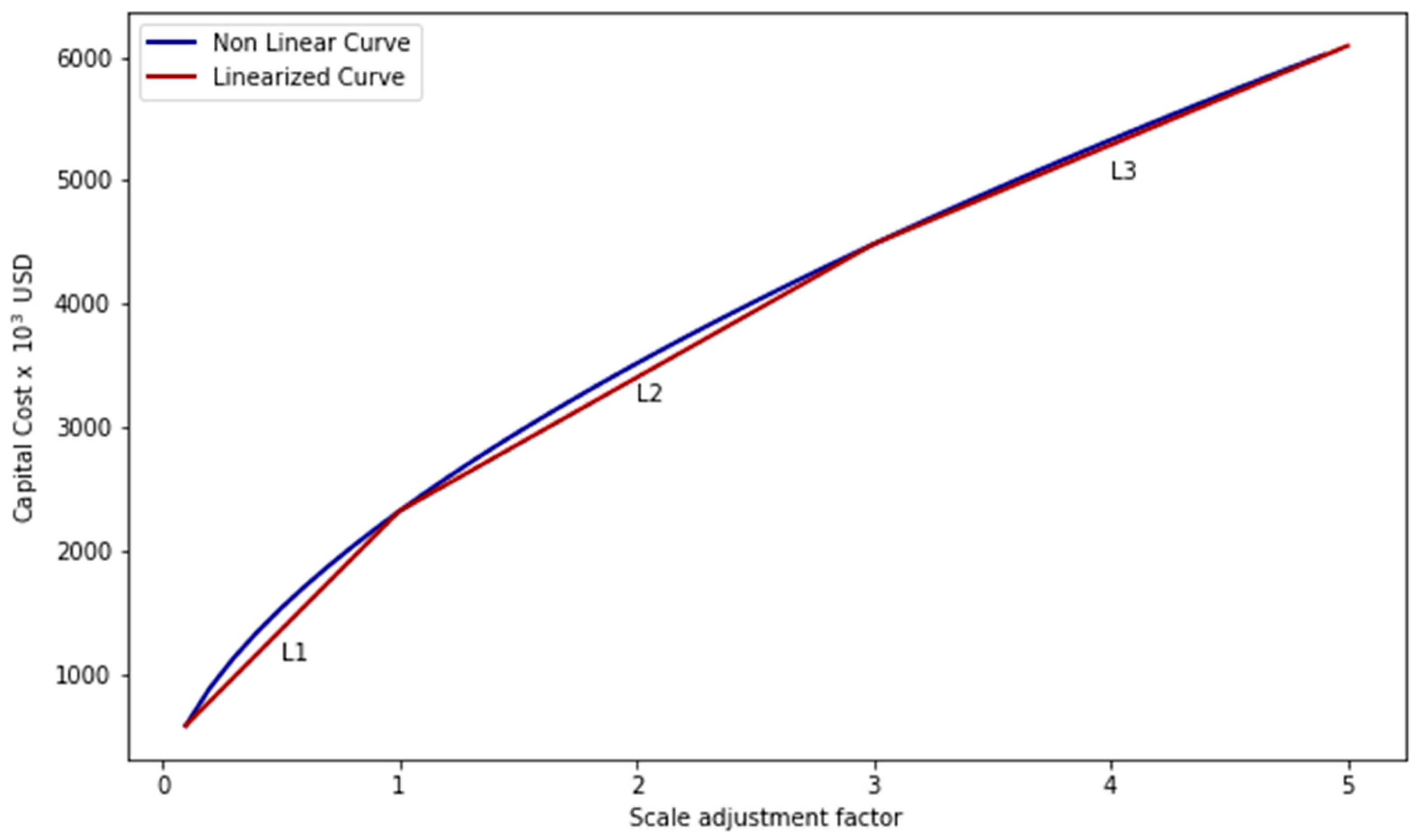
For ammonia production, it was considered that nitrogen would be obtained by the cryogenic distillation process of air, and ammonia production would be by the Haber–Bosch process. To calculate the total avoided CO₂ and consequently the carbon credit generated, the emitted and avoided CO₂ for each resource are provided in the Supplementary Materials (Table S2), as well as the IAR and OAR for each unit (Tables S3 and S4) and the process linearised cost curve. The following section will provide a more detailed description of the routes and scenarios, as well as the models used.

3.1. Evaluated Scenarios

3.1.1. Scenario 1

The objective of scenario 1 is to evaluate the potential of the sugarcane industry in the state of São Paulo to defossilise ammonia production. To this end, scenario 1 considers the construction of a new ammonia production plant with a capacity to meet a demand of 191,000 tons per year. This value is taken as a reference based on an existing ammonia plant in the state [27]. In both scenarios, the superstructure is free to choose the location of a new ammonia production plant and to organise the logistics of production and distribution of the necessary resources. To this end, an ammonia demand of 191,000 tons was added to each location considered, and an availability of vinasse, filter cake and ethanol was assumed. The availability of ethanol was determined by considering the sum of the installed capacity of the ethanol production plants present in that micro-region. This information was made available by the National Petroleum Agency (ANP) [28]. The availability of vinasse and filter cake was determined by considering that for each litre of ethanol produced, 12 L of vinasse and 0.45 kg of filter cake are generated [9]. The resource availability for ethanol, vinasse and filter cake for each place are provided in the Supplementary Materials (Table S5).

3.1.2. Scenario 2

As previously stated, scenario 2 is designed to assess the potential of the sugarcane industry in the state of São Paulo to defossilise ammonia production, with a particular focus on the optimisation of existing infrastructure. As in scenario 1, the demand for 191,000 tons of ammonia was used as a reference point. However, for the infrastructure to be used, several considerations were made. Regarding route 1, it was assumed that integration would occur through the supply of biomethane, considering the utilisation of the existing gas pipeline network and the deployment of established processes, including natural gas reforming, cryogenic air distillation and Haber–Bosch, all of which are situated in the city of Cubatão. In this sense, biomethane must be produced somewhere, transported to the gas pipeline and then delivered to the city of Cubatão. It has been considered that all the micro-regions through which the pipeline passes are potential injection sites for biomethane. The quantity of biomethane required to satisfy the demand for ammonia was determined based on [29,30,31]. Regarding route 2, it was postulated that the integration would occur through the supply of hydrogen, given that the conversion of ethanol into hydrogen is a process that still requires construction. The hydrogen demand was calculated based on [31]. The ethanol, vinasse and filter cake availability for scenario 2 were determined following the same procedure as scenario 1.

3.2. Hydrogen Production Routes

3.2.1. Biomethane Steam Reforming (Route 1—R1)

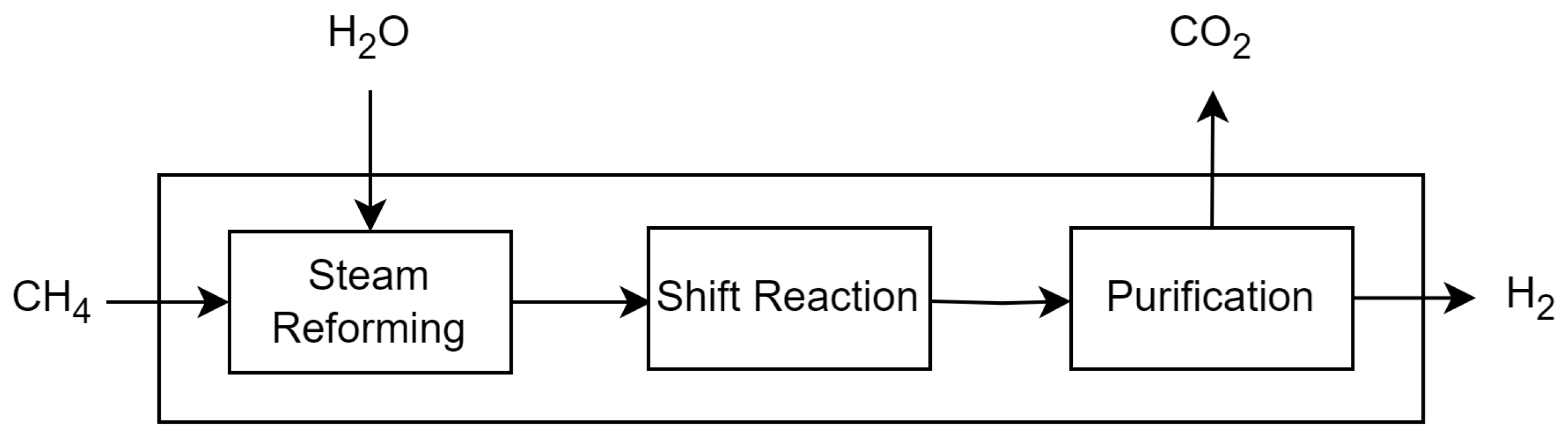
Route 1 looks at the biomethane steam reforming process. Biomethane can be obtained through two processes: vinasse biodigestion or filter cake biodigestion. In both processes, vinasse or filter cake is sent to anaerobic biodigesters, and all the biogas is sent for desulphurisation to remove H₂S. The pressure swing adsorption (PSA) process removes all the CO₂ in the biogas. Once the biomethane has been purified, it is sent to the steam reforming process, which has three main stages: steam reforming, water–gas shift reaction and hydrogen purification. Biomethane reacts with steam at high temperatures and produces carbon monoxide and hydrogen. The CO from the last step reacts with more steam water, making CO₂ and more H₂. Finally, the H₂ is purified using a PSA process, resulting in a high-purity hydrogen product. The data on converting vinasse and filter cake into biomethane and the investment costs were obtained from sources [9,32]. Information on the biomethane steam reforming process was obtained from sources [29,30]. Figure 3 and Figure 4 show a representation of each process.

3.2.2. Ethanol Steam Reforming (Route 2—R2)

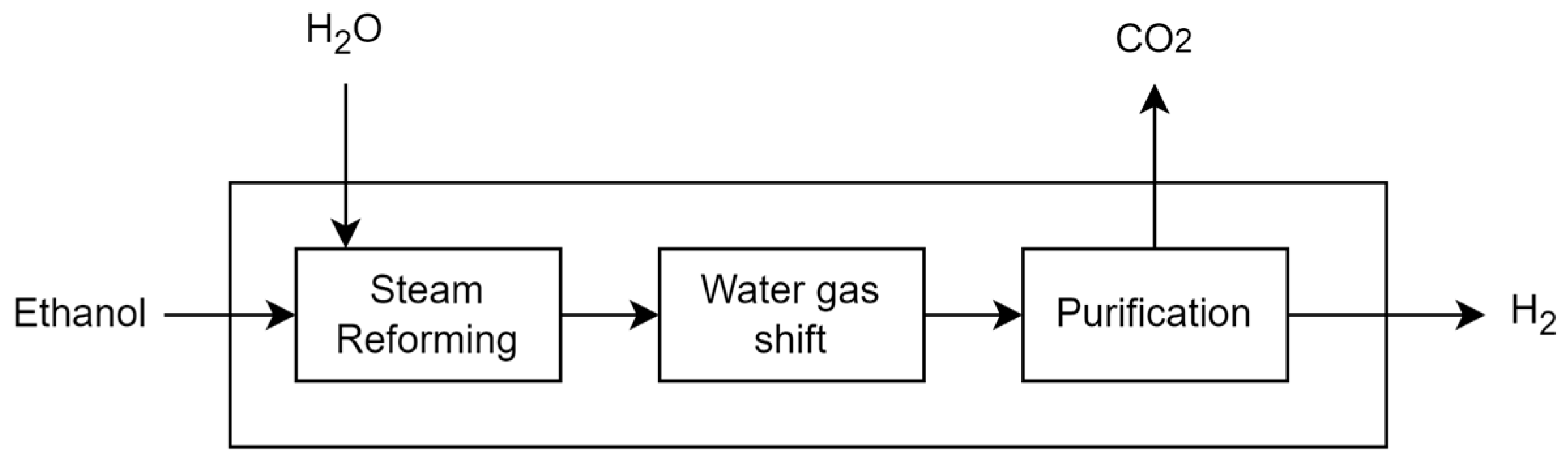
Route 2 considers hydrogen production through the ethanol steam reforming process, which consists of three main steps: steam reforming, water–gas shift reaction and hydrogen purification. Initially, ethanol (C₂H₅OH) is combined with steam (H₂O) in the presence of catalysts, producing hydrogen (H₂), carbon monoxide (CO) and carbon dioxide (CO₂). In the next step, CO reacts with steam in a water–gas shift reaction, producing additional hydrogen and CO₂. The gas mixture is then separated in a PSA process, resulting in a highly purified hydrogen output. The data used in this model were sourced from [33]. Figure 5 shows a representation of ethanol steam reforming process.

3.3. Auxiliary Processes

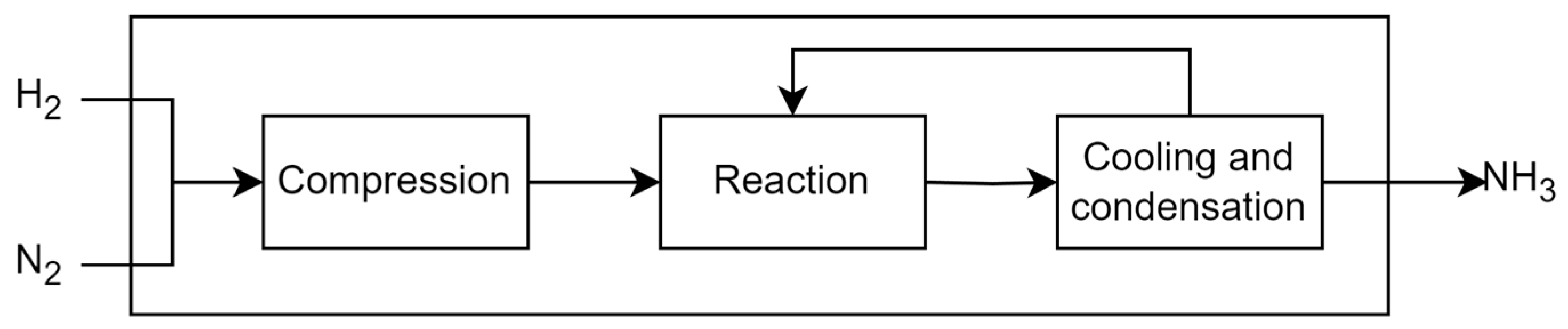
3.3.1. Haber–Bosch Process

The Haber–Bosch process is an industrial method developed in the early 20th century for making ammonia from hydrogen and nitrogen. The gases are mixed in a reactor under high temperature and pressure, in a catalyst presence [7]. The mixture is then cooled, and the ammonia becomes a liquid that is separated from the unreacted gases. The unreacted gases are returned to the reactor to improve efficiency. The liquid ammonia is then purified and stored under optimal conditions [6]. It can be used directly as a fertilizer or as a raw material for other nitrogen compounds. The model was constructed using economic and material balance information from sources [3,31], respectively. Figure 6 shows a representation of Haber-Bosch process.

3.3.2. Cryogenic Air Distillation

Cryogenic air distillation is a process used to separate the components of air, such as nitrogen and oxygen. This process has four stages: compression, refrigeration, cryogenic refrigeration and fractional distillation, as shown in Figure 7. Initially, atmospheric air is compressed to a high pressure (5–8 atmospheres) using compressors and then is cooled. In the cryogenic refrigeration stage, the air is cooled to cryogenic temperatures (between −185 °C and −190 °C). The cooled air is expanded, which makes it partially liquefy. In the fractional distillation stage, two columns separate the air components. The first column separates the air into an oxygen-rich fraction and a nitrogen-rich fraction. The final separation occurs in the low-pressure column. The pure oxygen exits the lower part of the column, while the pure nitrogen stream is obtained at the top. The model was constructed using information from [3].

3.4. Electricity Production

Usually, in conventional distilleries, the electricity is supplied by a cogeneration system that consumes a fraction of the produced bagasse. However, as the processes occurs outside the distillery, in the evaluated scenarios it is considered that the electricity is supplied by the electricity network available, with an acquisition cost of 65.00 USD.MWh⁻¹ and CO₂ emissions 0.1185 tonCO_2eq.MWh⁻¹ [34].

3.5. Resource Transportation

For all resources, it was assumed that transport could take place by truck. For the transport of biomethane in scenario 2, it was considered that it could also take place through the gas pipeline network. The costs and emissions for the transport of each resource are shown in the Supplementary Materials (Table S6).

3.6. Uncertainty Parameters

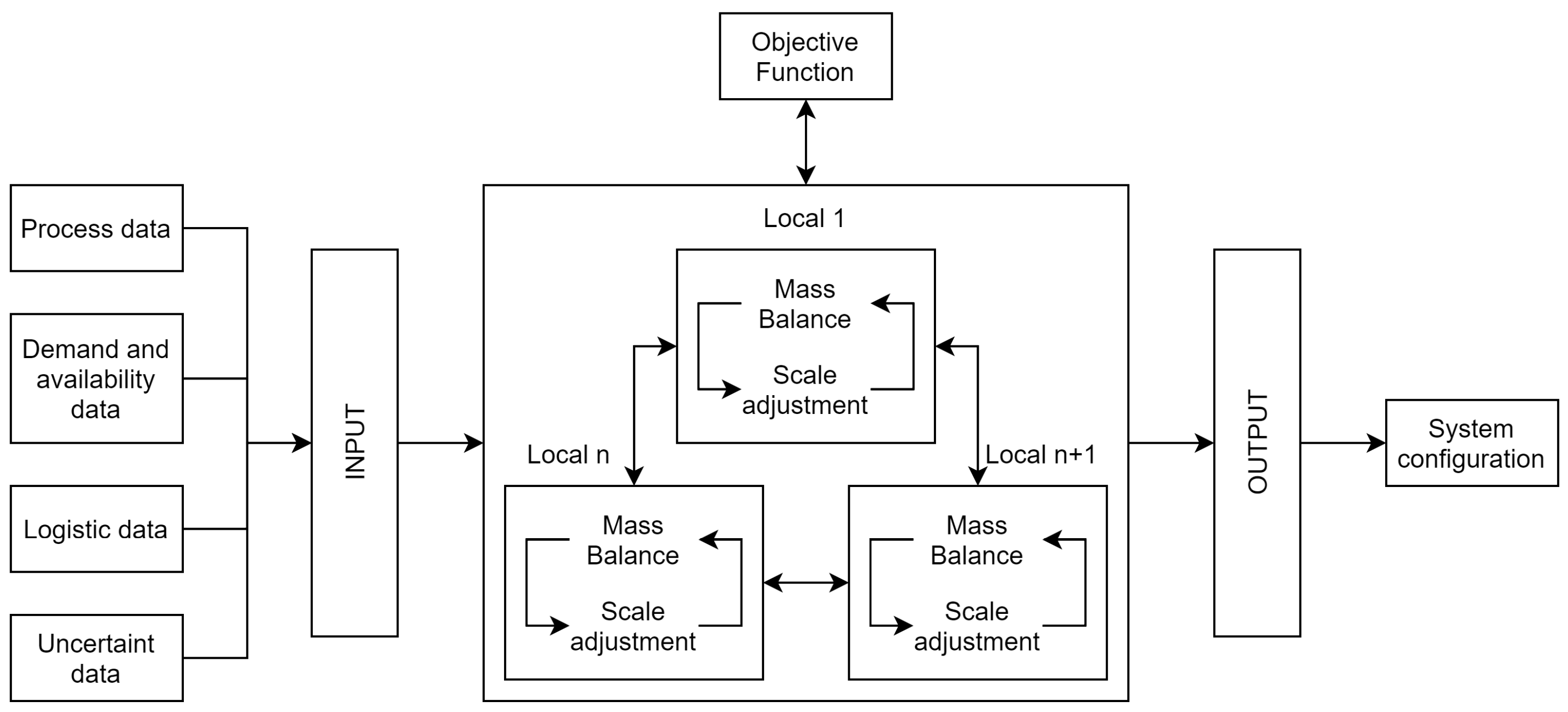
To consider the uncertainty present in purchase and sale prices and resource transportation costs, the robust optimisation method with box-type geometry was used to define the uncertain set. For each of the cases evaluated, a 20% disturbance, fpert and a psi of 0.4 were considered as te reference. In addition, different optimisation scenarios were performed, varying the degree of conservatism of the uncertain set through the value of psi.

3.7. São Paulo State Description

The state of São Paulo is the main producer of ethanol from sugar cane in Brazil, making a significant contribution to the national energy matrix. With its favourable climate and fertile soil, the state of São Paulo is home to 144 sugarcane mills, which are responsible for producing 36.8% of the country’s ethanol [28]. This production is complemented by a robust transport infrastructure, including some 199,000 km of highways for ethanol transport and a natural gas pipeline network that can be used to transport biomethane [35].

4. Results and Discussion

In this work, the model presented in Section 2 was used to assess the potential for defossilising ammonia production by integrating it with ethanol production. Two different cases were considered, each consisting of two routes. The first case aims to identify the micro-region in the state of São Paulo that would be most suitable for building a new ammonia plant, considering the availability of ethanol, vinasse and filter cake in each micro-region. The second case aims to understand how the production and logistics of biomethane and hydrogen should be organised to meet the existing demand for an ammonia production plant in Cubatão. The purchase and sale prices of resources are provided in the Supplementary Materials (Table S7).

Table 1. Objective function value obtained for the evaluated cases, considering different Ψ values.

Scenario	Route	Case	Ψ	Objective Function Value (USD)
1	Biomethane	1	0	2.357 × 108
			0.2	2.131 × 108
			0.4	1.905 × 108
			0.6	1.687 × 108
			0.8	1.453 × 108
			1	1.288 × 108
	Ethanol	2	0	8.51 × 107
			0.2	4.42 × 107
			0.4	7.99 × 106
			0.6	0
			0.8	0
			1	0
2	Biomethane	3	0	1.131 × 108
			0.2	1.105 × 108
			0.4	1.080 × 108
			0.6	1.054 × 108
			0.8	1.028 × 108
			1	1.003 × 108
	Ethanol	4	0	3.905 × 108
			0.2	3.396 × 108
			0.4	2.887 × 108
			0.6	2.378 × 108
			0.8	1.869 × 108
			1	1.361 × 108

presents the values obtained for the objective function for each of the cases evaluated, changing the degree of conservatism of the solution by controlling the size of the solution set, through the parameter Ψ. For the different values tested, except for case 2, there were no changes in the locations of the processes, which will be presented in the next paragraphs. In case 2, when restricting the solution space, no viable solutions were found, so the objective function presented a value equal to zero.

Table 2. Main economic results obtained for evaluated cases.

	TAC (MMUSD.year−1)	Investment (MMUSD)	Payback (year)
Case 1	237.2	3846.1	6.78
Case 2	90.5	314.9	3.19
Case 3	113.8	316.7	2.25
Case 4	391.8	259.2	0.64

presents the main economic results obtained for the evaluated cases, which will be commented on in the next paragraphs.

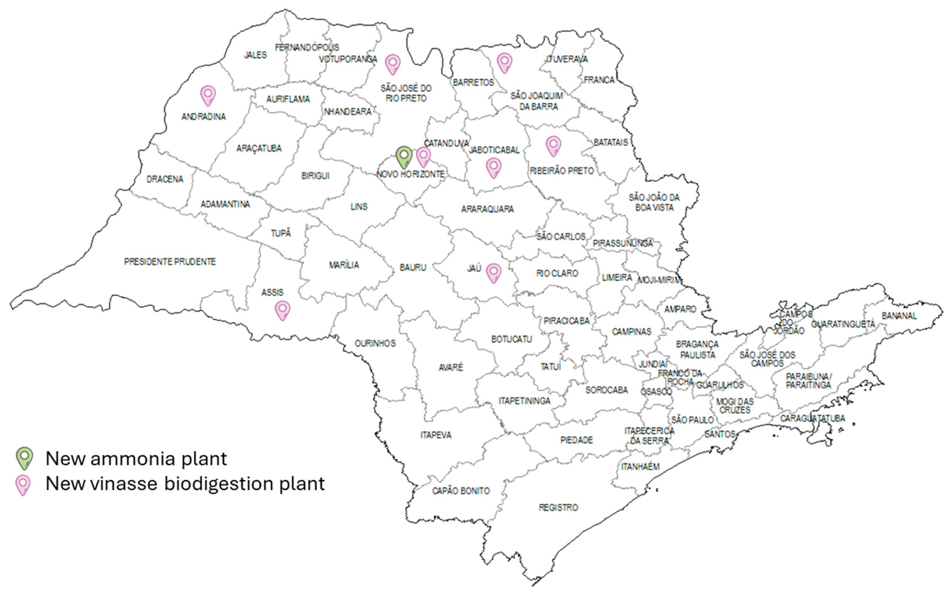
Figure 8 illustrates the spatial distribution of the production configuration and distribution of the resources required to meet ammonia demand in the state of São Paulo. The map illustrates that, while ammonia production is concentrated in Novo Horizonte, biomethane production is decentralised across eight locations, accounting for 54% of the total available vinasse. Upon evaluation of the availability of vinasse and the location of each biomethane-producing micro-region, it becomes evident that, except for Nova Horizonte, these are the seven locations with the greatest availability of vinasse. The selection of locations with the highest vinasse availability demonstrates the significance of reducing the investment cost per tonne of biomethane for the process’s viability. The decision to situate both a vinasse biodigestion plant and the other necessary ammonia production processes in Nova Horizonte can be viewed as a matter of logistics.

The map in Figure 8 shows that Nova Horizonte is in the centre of the other regions, reducing the cost of transporting biomethane between the biodigestion and reforming plants. In case of other locations having been chosen to concentrate ammonia production, biomethane processing would have been moved from the central region and its transportation costs would have increased. This shows that not only is the scale of the process important, but transport costs also have a major influence on the location of new plants. As with conventional ammonia plants, both the nitrogen, obtained through the cryogenic air distillation process, and the hydrogen, obtained through biomethane steam reforming, are produced in the same location as the Haber–Bosch process, thus avoiding the cost of transporting these resources. In this configuration, ammonia production had a TAC of USD 2.372 × 10⁸ and a total investment of 3307 × 10⁸ as shown in Table 2. The low payback time can be explained by the fact that the main resource in this case, vinasse and filter cake, has no acquisition cost. Given that these resources are waste and lack an established market for their commercialisation, it was assumed that they would have a zero-acquisition cost, thereby reducing raw material costs and the return on investment time. This is an avenue that the sector could pursue further.

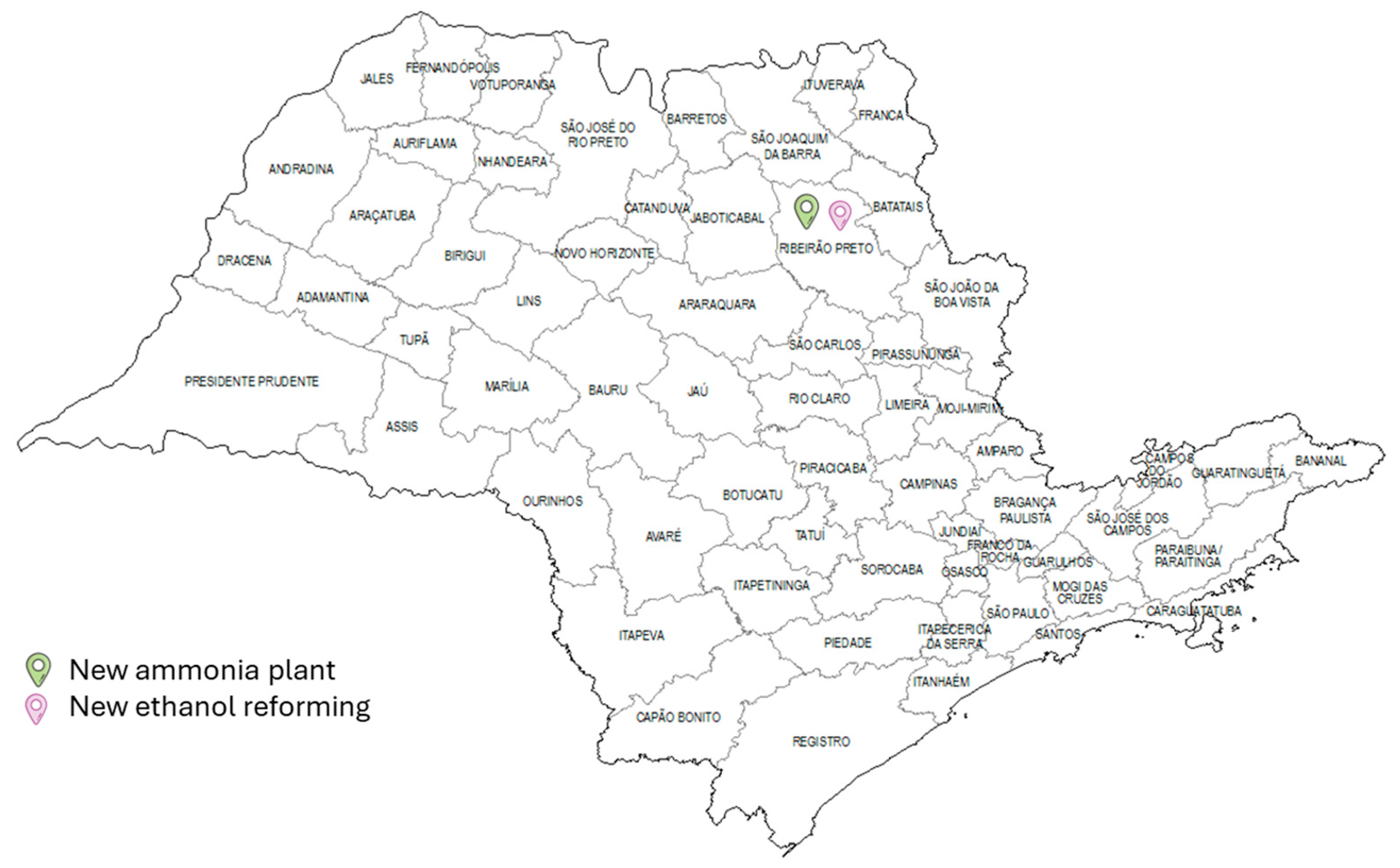
Figure 9 illustrates the location of the new plants for case 2, which features centralised processing for all resources, in contrast to case 1. The Ribeirão Preto micro-region was selected to house the processes needed to produce ammonia, due to its consumption of 1,022,602.28 m³ of ethanol, equivalent to 63 per cent of local availability and 8 per cent of the total. This figure represents 8 per cent of the total and is therefore relatively low. In addition to the ammonia plant, there is an air distillation plant to produce nitrogen. For this configuration, ammonia production had a TAC of 8.51 × 10⁷, with a total investment and ammonia revenue of USD 314 MM and USD 534 MM, respectively. In this case, the payback was 3.2 years.

When evaluating the consumption of available resources, the results indicate a significant difference between the two routes. The biomethane route consumes 54% of the vinasse available throughout the state, while route 2 consumes only 8% of the total volume of ethanol available. This discrepancy shows that the biomethane route requires greater mobilisation of the plants to meet the total demand for ammonia, making this route unlikely to be realised. In contrast, the ethanol route shows greater efficiency in terms of resource consumption.

A comparison of the two cases reveals that route 1 has a higher total annualised cost than route 2, making it a better option, considering the objective function. In contrast to ethanol reforming, steam reforming of natural gas is a more established and widely understood technology. Consequently, the utilisation of biomethane in lieu of natural gas will not necessitate substantial technological modifications, thereby reducing the cost of hydrogen production to a degree that is less than that that incurred by ethanol reforming. For the ethanol route, the cost of producing ammonia was USD 2746/tonne, whereas for the biomethane route it was USD 1880/tonne. Although route 1 has a longer payback period than route 2, it can be considered the most economically viable option. While the return on investment is quicker, case 2 has significantly higher raw material costs than case 1, which reduces the final balance for the period (income and expenses).

As indicated by [36], the estimated production cost of bio-based ammonia is within the range of USD 450 to USD 2000 per tonne, which is considerably higher than that of natural-gas-based ammonia and coal-based ammonia, which are within the range of USD 110 to USD 340 per tonne. Based on the values and the conditions evaluated, the production of ammonia integrated with ethanol production would result in uncompetitive ammonia. For this integration to be viable, it would depend on the creation of new markets, supported by different mechanisms. One potential mechanism for addressing this issue is the incorporation of a premium associated with the sustainable nature of the process into the price of ammonia. For the context under consideration, this premium would be USD 2500, based on an average market price for ammonia of USD 300 per tonne [37]. This results in a value of USD 2800, which is the figure considered in this work. Despite that, a widely used mechanism, especially in the transportation sector, is to establish mandates to replace fossil fuels with their renewable equivalents, as has been the case with sustainable aviation fuels and biodiesel. Actions along these lines could be taken for the use of fertilizers, so that all nitrogen fertilizers derived from ammonia should be produced in part with low-carbon ammonia.

Figure 10 illustrates the novel production configuration for case 3, wherein it is evident that biomethane production is characterised by a decentralised structure, with biodigestion of vinasse occurring in disparate locations, akin to the configuration observed in case 1. The total annualised cost for this configuration was found to be USD 1.13 × 108, representing a 53% reduction compared to that of case 1. The total investment in this case was USD 316 million, with revenue obtained from supplying biomethane amounting to USD 50.5 million. The ability to take advantage of the biomethane reforming unit meant that the payback period for this configuration was 2.25 years, representing a reduction of 4.5 years compared to that of case 1.

Upon analysis of vinasse consumption, it was determined that the quantity consumed was equivalent to that observed in case 1 (84,493,285 tonnes). Additionally, it was established that 100% of the vinasse available in Ribeirão Preto, Andradina, Jaboticabal, Jaú, Assis, Araçatuba and Limeira was consumed, while in São Joaquim da Barra, the consumption was 95%. Except for São José do Rio Preto, biomethane production occurred in the nine cities with the greatest availability of vinasse. Despite its availability, filter cake was not consumed in any of the towns, which can be attributed to the lower availability of this resource. While filter cake has a higher generation potential per unit of mass (filter cake: 41.5 Nm³/ton of substrate; vinasse: 6.6 Nm³/ton of substrate [38]), its smaller available volume results in a higher total biomethane generation cost than if vinasse were used. It was thus demonstrated that the production of biomethane through the biodigestion of vinasse was a more attractive proposition in the context under consideration. Even though biomethane production occurs at the same injection site in Andradina, Araçatuba and Limeira, Rio Claro, Araraquara and Lins locations were supplied by production in the cities of Jaú, São Joaquim da Barra and Assis, respectively, while São Carlos is supplied by production in the micro-regions of Ribeirão Preto and Jaboticabal. The greatest distance travelled between these cities was between São Joaquim da Barra and Araraquara, at 161 km. Given that the Birigui micro-region had vinasse and was one of the micro-regions with direct access to the gas pipeline, it was not included in the biomethane production system. The limited availability of resources in this location would necessitate a reduction in the scale of the process, resulting in a considerably higher production cost than in other regions. It can thus be seen that, in addition to proximity to the natural gas distribution network, the availability of resources at the selected biomethane production and injection sites was an important factor in the decision-making process.

Figure 11 illustrates the configuration of the ethanol distribution network, which is designed to meet the hydrogen consumption requirements of the ammonia production facility situated in Cubatão. The configuration demonstrates that, although ethanol is supplied from disparate locations, hydrogen production through ethanol steam reforming is concentrated in the city of Cubatão, situated within the Santos micro-region. The total annualised cost of hydrogen production in this configuration was USD 3,905,000,000. Similarly, the centralisation of the ethanol-to-hydrogen conversion process was also observed in case 2. However, in case 2, the Ribeirão Preto micro-region had all the ethanol it required, thus obviating the expense of transporting this resource from other regions.

In case 4, the total investment amounted to USD 259 million, while the cost of raw materials reached USD 474 million. Consequently, the cost of centralised hydrogen production was determined to be USD 3.627 per kilo of hydrogen. The cost of producing hydrogen would increase by 36.47% if production were to take place in a decentralised way, with ethanol being converted in its various places of origin and the hydrogen produced transported to Cubatão. Despite the total investment required being only 30.6% higher, the logistical cost is increased by 311% due to the transportation of hydrogen. Therefore, in addition to the issues of availability and distance of ethanol to the consumer’s location, the resource transported also had an influence on the structure of the supply network. Of all the cases evaluated, this was the one with the lowest payback period. This can be explained by the combination of different factors, such as the lower cost of centralised production and the high price of the product.

5. Conclusions

The proposed formulation was used to evaluate the feasibility of integrating low-carbon ammonia production with ethanol production in the state of São Paulo, Brazil. While other studies have used MILP formulations with robust optimisation to evaluate different production configurations, no studies were identified that specifically addressed the integration of low-carbon ammonia production with ethanol production. In this context, several cases were investigated, varying the integration route and the scenario considered. The results suggest that despite the financial competitiveness of the biomethane route, the defossilisation of ammonia production via this route would be more challenging than via the ethanol route. The ethanol route necessitates the utilisation of merely 8% of the ethanol present within the entire state and can be supplied by a single site. In contrast, the biomethane route would consume 54% of the available vinasse, necessitating a greater mobilisation of the sector to produce renewable ammonia. In this sense, it is possible to note a greater potential for the ethanol route than the Biomethane route. However, future, more in-depth studies are needed to better assess other aspects such as the environment, other technologies and routes. The results also suggest that the location of the consumer has a significant impact on the choice of location, as does the availability of the resource. The results presented here can be used to inform and underpin more detailed studies in the regions and configurations presented and subsequently to inform the development of instruments and local public policies that promote the production of low-carbon ammonia integrated with ethanol production.