Effects of the Characterization Methods of Heptane Plus Components (C7+) on the Phase Behavior of Volatile Fluids

Abstract

For reservoir fluids with strong volatile tendencies, such as gas condensate and volatile oil, the determination of the characteristic parameters of the equation of state has a great influence on the fluid phase behavior and subsequent reservoir engineering, production engineering, and surface facilities design calculations. However, the process of characterizing reservoir fluid lacks a unified and standardized procedure, and the methods are largely empirical and rather complicated. In this paper, three main stages are defined for the characterization of the equation of state parameters for these volatile reservoir fluids, including (1) determining the C7+ distribution, (2) calculating the equation of state parameters for the C7+ single-carbon component, and (3) lump components. The typical calculation methods in each step and their effects on the fluid phase behavior calculations are quantitatively analyzed and compared. Finally, the workflow and the suitable characterization methods for gas condensate and volatile oil phase behavior calculations are selected. The results show that C7+ distribution and C7+ single carbon component properties have a greater influence on the phase behavior prediction of condensate gas and volatile oil, while the lumping of C7+ single carbon component has relatively little influence.

1. Introduction

Reservoir fluid is a complex mixture. The lighter (such as CH₄, N₂, CO₂, and H₂S) and mid-weight components (such as C₂ to C₆) can be clearly defined through experiments for their equation of state (EOS) characteristic parameters, such as critical temperature ($T_{ci}$), critical pressure ($P_{ci}$), molecular weight ($M_{wi}$), acentric factor (${\omega }_i$), volume transfer parameters ($v_{si}$), etc. However, many heavier components (such as C₇₊) are difficult to clearly classify into a specific component. They are mixtures under high-temperature and high-pressure conditions. The distribution and relative amount of C₇₊ components in the reservoir fluid have significant effects on the PVT (Pressure–Volume–Temperature) properties and phase behavior of the reservoir fluid [1].

The determination of characteristic parameters for heavy components (C7+ or C11+) in reservoir fluids significantly influences the PVT properties and phase behavior predictions of the fluids. For example, the presence of heavier C7+ components increases the overall density and viscosity of the fluid, shifts critical points and the phase envelope of the fluids, and modifies the gas-to-oil ratio at the surface conditions.

Consequently, heptane plus characterization greatly impacts the prediction results for reservoir performance, production curve, and surface facilities engineering [2]. Additionally, the contribution of C7+ characterization is also important in the drilling engineering compositional modeling and dynamic wellbore flow simulation [3,4]; it is also needed in modern scientific process simulators [5]. When calculating the PVT properties and phase behavior of reservoir fluids, cubic equation of state (EOS) such as Peng–Robinson (PR) [6] and Soave–Redlich–Kwong (SRK) [7] are commonly used in the oil and gas industry. These types of EOS models require the definition of the total number of components and the characteristic parameters of each component (such as molecular weight, critical point, and acentric factor) for fluid PVT and phase behavior calculations [8]. Therefore, it is crucial to clearly define the splitting and lumping schemes for heavy components (C7+ and C11+) and determine the characteristic parameters of the resulting pseudo-components before any EOS calculations can be performed. To address these needs, the primary issues that must be resolved in EOS modeling are as follows:

(1)

When detailed gas chromatography experimental data are available, the component distribution of single carbon number (SCN) mixtures ranging from C7 to C36+ can typically be obtained. However, the number of chromatographic components is often excessive, and the direct application of experimental composition data in engineering calculations can significantly increase simulation time. Therefore, lumping the SCN components derived from gas chromatography into several pseudo-components will greatly improve computational efficiency. This raises the question: which lumping method best represents the phase behavior and PVT properties of the original fluid?

(2)

In the absence of gas chromatography experimental data, heavy components in reservoir fluids are usually represented as a single component (C7+ or C11+). The mole fraction of this single heavy component can account for over 50% of the entire reservoir fluid. This single lumped component does not accurately represent the heavy component distribution within the reservoir fluid. Consequently, it is necessary to split the single C7+ component to gain a more detailed understanding of the heavy component distribution. Splitting involves using a specific probability distribution method to divide the single C7+ component into multiple single carbon groups (SCNs). Representing the entire C7+ component using the SCN group distribution enables a more accurate characterization of the phase behavior and PVT properties of the reservoir fluids. The components obtained after splitting can be further lumped into several pseudo-components to minimize the total number of components. The critical question is: which method of splitting and lumping can best represent the phase behavior and PVT properties of the original fluid?

(3)

After splitting and lumping SCN components, it is necessary to determine the EOS characteristic parameters (such as molecular weight, critical point, and acentric factor) of the resulting pseudo-components. Which methods can reliably obtain the characteristic parameters of these pseudo-components?

(4)

How significantly do different methods of splitting and lumping, as well as the calculation methods for the EOS characteristic parameters of the pseudo-components, impact the PVT properties and phase behavior calculation results of reservoir fluids?

In summary, we are left with three main questions: (1) Which component distribution model best represents the composition of real reservoir fluids? (2) Which methods for estimating the EOS parameters of the SCN group perform best in calculating hydrocarbon phase behavior? (3) Which lumping scheme or method has the least influence on the phase behavior of the hydrocarbon system before and after lumping? This paper attempts to address these questions through theoretical and methodological research, along with a comparison of various C₇₊ characterization methods. By conducting quantitative analysis and comparison of phase behavior calculations, we propose a clearly defined workflow for heavy component characterization, particularly for volatile oil and gas condensate.

2. C₇₊ Characterization Methods

The objective of C₇₊ characterization is to determine the characteristic parameters ($T_{ci}$, $P_{ci}$, ${\omega }_i$, $M_{wi}$, etc.) of the EOS so that the calculations accurately represent the phase behavior and physical properties of the reservoir fluids. After obtaining the PVT experimental report, if the report provides detailed component distribution (typically up to C₃₆₊), it is generally unnecessary to perform C₇₊ component splitting or predict the distribution of the components. Consequently, empirical correlations can be used to directly determine the EOS parameters for each single carbon number (SCN) group listed in the experimental report.

When the component analysis in the experimental report is relatively coarse (e.g., treating components above C₇₊ or C₁₁₊ as a whole), achieving more precise EOS simulation results often requires splitting the heavier components using an appropriate probability distribution model. This process yields the SCN component distribution pattern, from which the EOS characteristic parameters for these SCN groups can be determined using suitable empirical correlations.

Once the SCN component distribution and their characteristic parameters are clearly defined, appropriate lumping methods and mixing rules can be applied to combine the SCN groups into several pseudo-components, reducing the total number of components in the EOS model. The lumped reservoir fluid model must be tuned with PVT experimental data for further fitting and adjustment of the pseudo-component EOS characteristic parameters, resulting in EOS parameters that accurately represent the reservoir fluids. For a detailed workflow, refer to Figure 1.

In the workflow depicted in Figure 1, there are four clearly defined stages that significantly influence the final determination of EOS parameters. These stages are the following. (1) Obtain C₇₊ Splitting and Distribution: This stage involves determining how the heavy components (C₇₊) are split and distributed, which is essential for accurate EOS modeling; (2) Estimate EOS Characteristic Parameters for SCN Groups: This stage focuses on defining the EOS parameters—such as critical pressure, critical temperature, acentric factor, and molecular weight—for SCN groups; (3) Lumping of SCN groups: This step involves combining SCN groups using appropriate mixing rules to reduce the total number of components in the EOS model while maintaining the accuracy of the phase behavior and PVT properties calculation; (4) Pseudo-Component EOS Parameters Tuning: This step adjusts the pseudo-component parameters to align the EOS calculation results with the experimental PVT data. The methods and procedures used in this step are beyond the scope of this study. Next, we use representative methods and models from the literature to compare and analyze each of the first three stages individually.

2.1. Heptane Plus (C7+) Splitting and SCN Distribution Models

There has been extensive previous research on the splitting and distribution patterns of recombined components. The splitting models proposed by Pedersen et al. [9,10,11] and Whitson [12,13] are among the most widely used [14,15]. This study primarily employs these two models for component splitting research.

2.1.1. Pedersen’s Model

Based on the observation of the component distribution of a large number of reservoir fluids worldwide, Pedersen et al. [9,10,11] found that the distribution of components above C7+ exhibits the following linear relationship:

$$C_{\mathrm{N}\mathrm{i}}=A+B \mathrm{l}\mathrm{n}\left(z_{\mathrm{i}}\right)$$

(1)

Among them, $C_{\mathrm{N}\mathrm{i}}$ is the number of single carbons of the i-th C₇₊ component after splitting, and $z_{\mathrm{i}}$ is the mole fraction corresponding to this component. A and B are undetermined constants that can be determined by the lightest few C₇₊ components. Once A and B are determined, the remaining single carbon C₇₊ components $C_{\mathrm{N}\mathrm{i}}$ and their mole fractions $z_{\mathrm{i}}$ can be determined by Equation (1). All single carbon C₇₊ components obtained by splitting must satisfy the following material balance relationship:

$$z_{c7+}=\sum _{i=1}^N{z}_i$$

(2)

$$M_{c7+}={\displaystyle \frac{{\sum }_{i=1}^N{z}_i{M}_i}{{\sum }_{i=1}^N{z}_i}}$$

(3)

In Equations (2) and (3), $z_{c7+}$ and $M_{c7+}$ represent the mole fraction and the average molecular weight of the C₇₊ fraction in the reservoir fluid, respectively; $z_i$ and $M_i$ are the mole fraction and molecular weight of the splitted SCN group; and N is the total number of SCN components after splitting. Additionally, the density of the SCN component after splitting often increases with the increase in the number of carbons. Therefore, Pedersen expressed the density of the SCN component after splitting as

$${\rho }_{\mathrm{N}i}=C+D \mathrm{l}\mathrm{n}\left(C_{Ni}\right)$$

(4)

In Equation (4), C and D are constants that can be obtained from experimental data through linear trend line fitting. After splitting, the density of the SCN group must satisfy the material balance relationship as follows:

$${\rho }_{\mathrm{N}i}={\displaystyle \frac{{\sum }_{i=1}^N{z}_i{M}_i}{{\sum }_{i=1}^N\frac{z_i{M}_i}{{\rho }_i}}}$$

(5)

where

$$M_i=14C_i-4$$

(6)

2.1.2. Whitson’s Model

Whitson represents the distribution of SCN groups varying with molecular weight as the probability density function of molecular weight [12,13], as follows:

$$p\left(M\right)={\displaystyle \frac{{\left(M-\eta \right)}^{\alpha -1}exp\left\{-\left[M-\eta \right]/\beta \right\}}{{\beta }^{\alpha }\mathsf{\Gamma }\left(\eta \right)}}$$

(7)

where $\eta$ is the minimum molecular weight in the C₇₊ fraction distribution (typically $\eta$ = 92); M is the average molecular weight of the SCN group; and $\mathsf{\Gamma }\left(\eta \right)$ is the gamma function with the minimum molecular weight as the variable, which can be calculated using numerical methods. When the variable of the gamma function is 0 ≤ x ≤ 1, the gamma function can be approximated as

$$\mathsf{\Gamma }\left(x+1\right)=1+\sum _{i=1}^8{a}_i{x}^i$$

(8)

When the variable x in $\mathsf{\Gamma }\left(x\right)$ is greater than 1, its value can be obtained from the recurrence relation $\mathsf{\Gamma }\left(x+1\right)=x\mathsf{\Gamma }\left(x\right)$. The values of the fitting parameters ($a_i$) in Equation (8) can be found in

Table 1. Parameters for calculating the Gamma function in Equation (8).

Parameters	Value
$a_1$	−0.577191652
$a_2$	0.988205891
$a_3$	−0.897056937
$a_4$	0.918206857
$a_5$	−0.756704078
$a_6$	0.482199394
$a_7$	−0.193527818
$a_8$	0.035868343

.

α and β are adjustable parameters that define the shape of the probability distribution.

$$\beta ={\displaystyle \frac{M_{c7+}-\eta }{\alpha }}$$

(9)

$$\eta =14n-6$$

(10)

In Equation (10), n is the number of carbon atoms in the lightest SCN group of C7+ components (e.g., n = 7 or n = 8). When determining the mole fraction of a certain C7+ component, assuming its molecular weight lies between M1 and M2, the probability of occurrence of that component ($f_i$) is obtained by integrating the probability density function (Equation (7)) from M₁ to M₂ and then multiplying by the total mole fraction of the C7+ components in the fluid. The integral of the probability density function can be obtained as follows [9]:

$$P\left(M\le x\right)={\int }_{\eta }^{x}p\left(x\right)dx=e^{-y}\sum _{j=0}^{\infty }{\displaystyle \frac{y^{\alpha +j}}{\mathsf{\Gamma }\left(\alpha +j+1\right)}}$$

(11)

where $y=\left(x-\eta \right)/\beta$; when calculating Equation (11), the summation can be terminated given that the following conditions are satisfied:

$${\displaystyle \frac{y^{\alpha +j}}{\mathsf{\Gamma }\left(\alpha +j+1\right)!}}<{10}^{-7}$$

(12)

From Equation (11), the probability ($f$) of a C₇₊ component with a molecular weight between M₁ and M₂ is

$$f_i={\int }_{M1}^{M2}p\left(x\right)dx=P\left(M\le M2\right)-P\left(M\le M1\right)$$

(13)

$$z_i=f_i{·z}_{c7+}$$

(14)

Finally, when the molar fraction ($z_i$) and molecular weight ($M_i$) of the existing experimental SCN group distribution are available, Whitson suggests using the following empirical formula (Equations (15)–(17)) for calculating the adjustable parameter α [12,13]:

$$\alpha =Y^{-1}\left(0.5000876+0.1648852Y-0.0544174Y^2\right)$$

(15)

$$Y=\mathrm{l}\mathrm{n}\left[{\displaystyle \frac{M_{C7+}-\eta }{m_G}}\right]$$

(16)

$$m_G={\left[\prod _{i=n}^N{\left(M_i-\eta \right)}^{z_i}\right]}^{1/z_{c7+}}$$

(17)

If there are no experimental data, the α parameter value can be manually adjusted, typically ranging from 0.5 to 3.0 [12,13]. Compared to the Pedersen model, the Whitson model, based on probability density distribution theory and featuring an adjustable α parameter, offers greater flexibility and accuracy in predicting the distribution of heavy components in oil and gas systems.

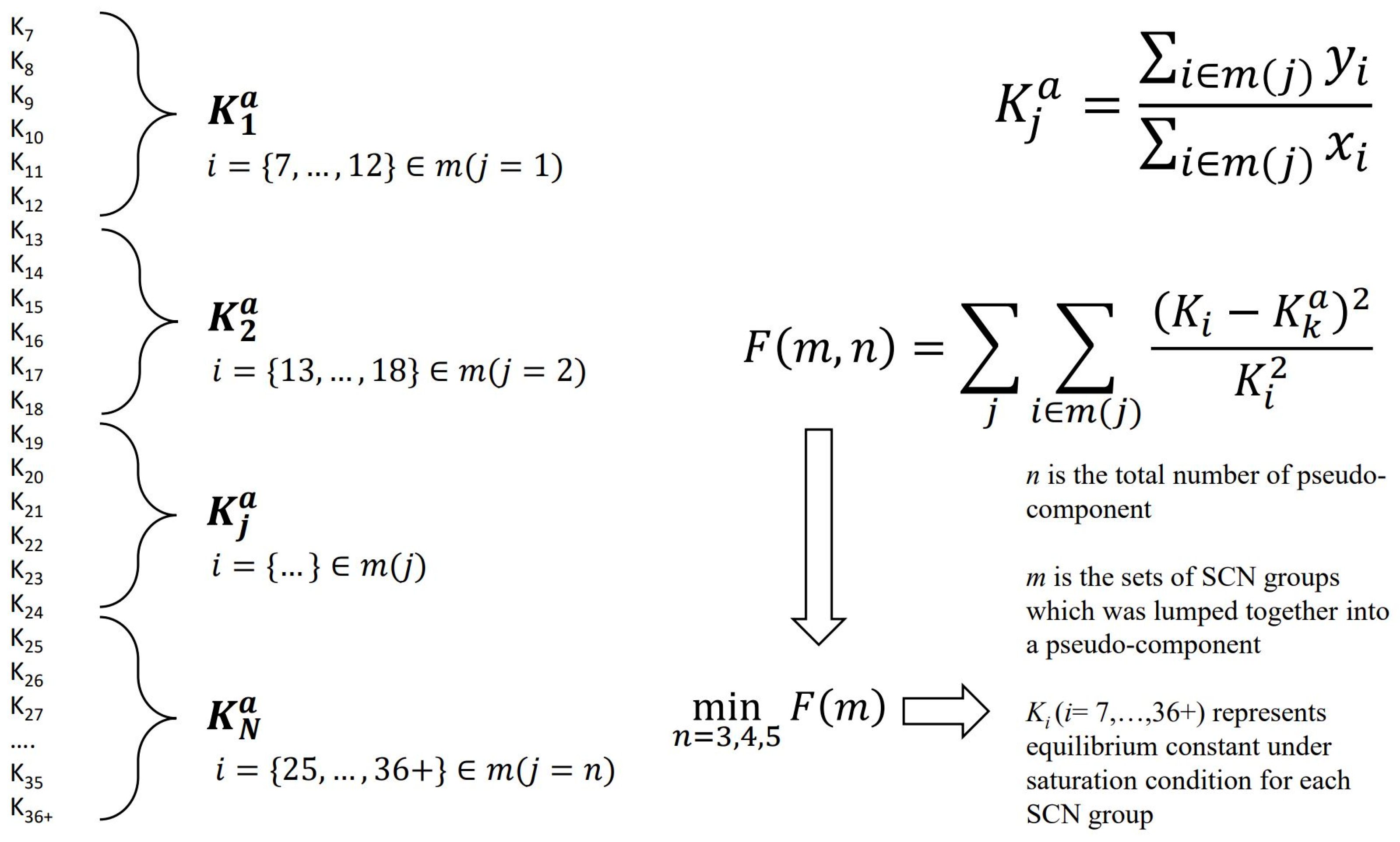
2.2. SCN Group EOS Parameters Estimation

The main objective of determining the EOS characteristic parameters for SCN groups is to estimate the critical pressure ($P_{ci}$), critical temperature ($T_{ci}$), acentric factor (${\omega }_i$), and other EOS parameters for the SCN groups after splitting. A significant amount of research has been conducted in this area [16,17,18,19,20,21,22,23,24], providing numerous empirical formulas for calculating EOS characteristic parameters. However, there is currently a lack of detailed discussion on the impact of EOS parameters obtained from various methods on the phase behavior of reservoir fluids. We consider the following methods for calculating SCN group EOS parameters (as shown in

Table 2. Methods for calculating EOS parameters for the SCN group.

Methods	Input	Output
1. Silva and Rodriguez [16]	$M_i$	${\gamma }_{c7+}$$,T_b$
2. Riazi and Daubert [17]	$M_i$$, {\gamma }_{c7+}$	$P_{ci}$$,T_{ci}$$,v_c$$,T_b$
3. Cavett [16]	${\gamma }_{c7+}$$, T_b$	$P_{ci}$$,T_{ci}$
4. Kesler and Lee [16]	${\gamma }_{c7+}$$, T_b$	$P_{ci}$$,T_{ci}$$,M_i$$,{\omega }_i$
5. Winn–Sim–Daubert [18]	${\gamma }_{c7+}$$, T_b$	$P_{ci}$$,T_{ci}$$,M_i$
6. Watansiri–Owens–Starling [19]	${\gamma }_{c7+}$$, T_b$$, M_i$	$P_{ci}$$,T_{ci}$$,v_c$$,{\omega }_i$
7. Edmister [16]	$P_{ci}$$, T_{ci}$$, T_b$	${\omega }_i$
8. Rowe [20]	$M_i$	$P_{ci}$$, T_{ci}$$, T_b$
9. Willman and Teja [21]	SCN	$P_{ci}$$, T_{ci}$$, T_b$
10. Magoulas and Tassios [22]	$M_i$$, {\gamma }_{c7+}$	$P_{ci}$$,T_{ci}$$,{\omega }_i$
11. Twu [23]	$M_i$$, {\gamma }_{c7+}$	$P_{ci}$$,T_{ci}$$,v_c$$,{\omega }_i$$, T_b$
12. Sancet [24]	$M_i$	$P_{ci}$$, T_{ci}$$, T_b$

Note: $M_i$, ${\gamma }_{c7+}$, $P_{ci}$, $T_{ci}$, v_c, ω_i, and T_b represent molecular weight, specific gravity, critical pressure, critical temperature, critical volume, acentric factor, and boiling point of the SCN group, respectively.

).

2.3. SCN Group Lumping and Corresponding Mixing Rule

The lumping of the SCN group involves combining multiple C7+ SCN components into a single C7+ pseudo-component. The aim is to minimize the number of components in the compositional model calculations for reservoir engineering. During the lumping process, two issues typically arise: (1) selecting the lumping boundary of SCN group so that a certain amount of SCN components can be lumped to most accurately represent the PVT properties and phase behavior of the original fluid and (2) determining which mixing rule to use for calculating the EOS parameters of the obtained pseudo-component. A significant amount of work has been conducted in this area [12,13,25,26]. We primarily select the Whitson method [12] and the Newley–Merrill method [25] for the lumping of single carbon number (SCN) components and conduct a comparative simulation study. The Whitson lumping method is straightforward to implement, whereas the Newley–Merrill method involves more complex calculations. However, the results indicate that the critical points and phase envelopes of the fluids obtained after lumping with both methods show minimal differences compared to those before lumping. The Hong’s mixing rule [26] is used throughout the lumping process of this study.

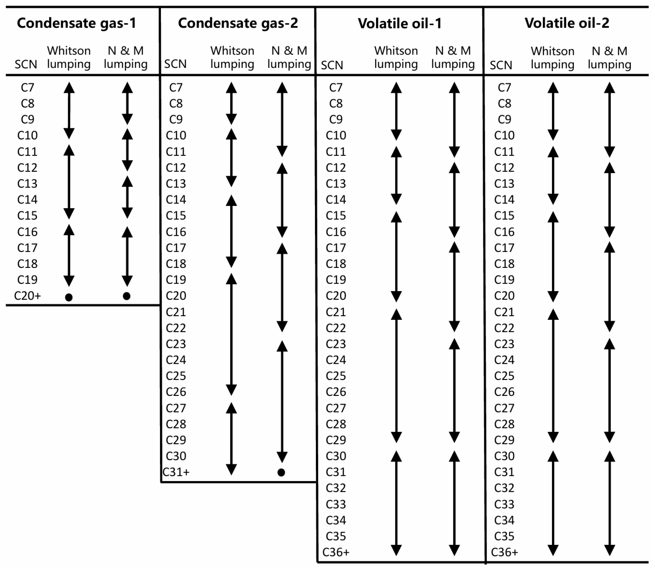
2.3.1. Whitson Lumping Methods

The Whitson method [12] can lump C7+ single carbon number (SCN) components with a certain composition distribution into several multi-carbon number (MCN) pseudo-components. The number of MCN pseudo-components (N_{MCN}) can be expressed by an empirical equation as follows:

$$N_{\mathrm{MCN}}=\mathrm{Int}\left[1+3.3\log \left(N-n\right)\right]$$

(18)

In Equation (18), the function Int represents the integer part (rounding down) and N and n represent the maximum and minimum number of carbon atoms in the single carbon number (SCN) distribution, respectively. After obtaining N_{MCN}, the molecular weight boundary values for each MCN pseudo-component (M_I, I = 1, 2, \ldots, N_{MCN}) can be estimated as follows:

$$M_I=M_{C7}{\left({\displaystyle \frac{M_{N+}}{M_{C7}}}\right)}^{I/N_{MCN}}$$

(19)

$M_{N+}$ represents the maximum molecular weight in the SCN distribution and $M_{C7}$ represents the molecular weight of C7 (which can be taken as the constant 96). For example, if the calculated $N_{MCN}$ = 4 and $M_I$ = {121, 167, 232, 314}, then the original C7+ SCN distribution is divided into four MCN pseudo-components, with each pseudo-component having a molecular weight range of 96–121, 122–167, 168–232, and 233–314, respectively.

2.3.2. Newley–Merrill Lumping Methods

The main idea of the Newley–Merrill [25] method for lumping SCN groups into several pseudo-components is to construct an objective function through equilibrium constants. This objective function reflects the differences in equilibrium constants of each component before and after the lumping into pseudo-components. The pseudo-component lumping scheme is obtained when this objective function reaches its minimum value. To the best of our knowledge, we found that the Newley–Merrill method performs better than the traditional lumping schemes based on empirical formulas because of the following two reasons: (1) the phase diagram of the fluid remains essentially unchanged before and after lumping, meaning that the fluid SCN groups lumped into fewer MCN pseudo-components essentially retains the phase diagram of the original fluid and (2) the deviation of the fluid’s critical point before and after lumping is quite small. The technical approach of the Newley–Merrill method [25] is shown in Figure 2. The drawback of this method is that the calculation process is relatively complex.

2.3.3. Hong’s Mixing Rule

In our previous research [27], we found that the Hong’s mixing rule provides better results for calculating the EOS parameters of MCN pseudo-components compared to the Newley–Merrill [25] mixing rule. Therefore, we have selected the Hong’s mixing rule for the estimation of pseudo-components EOS properties. The weighting factor ($w_i$) of Hong’s mixing rule is defined as follows:

$$w_i={\displaystyle \frac{z_i{M}_i}{{\sum }_{i\in L}^L{z}_i{M}_i}}$$

(20)

In Equation (20), L (as a superscript or subscript) represents a certain MCN pseudo-component obtained after the lumping of SCN components and i represents the i-th SCN component within that MCN pseudo-component. Based on the weighting factor defined in Equation (20), the EOS parameters ${\mathsf{\Theta }}_{cL}$ of the lumped MCN pseudo-components (which can represent the pseudo-critical pressure $P_{cL}$, pseudo-critical temperature $T_{cL}$, pseudo-critical molar volume $v_{cL}$, acentric factor ${\omega }_L$, and molar mass $M_L$) can be expressed as

$${\Theta }_{cL}=\sum _{i\in L}^L{w}_i{\Theta }_{ci}$$

(21)

The binary interaction parameter after lumping ($k_{ijL}$) is

$$k_{ijL}=1-\sum _{i\in L}^L\sum _{j\in L}^L{w}_i{w}_j\left(1-k_{ij}\right)$$

(22)

where $k_{ij}$ is the binary interaction parameter of SCN group from the van der Waals single fluid mixing rule.

3. Fluids Description

In this study, four oil and gas samples (two condensate gas samples and two volatile oil samples) were selected for comparative calculations. The experimental component data from the PVT reports can be found in

Table A1. Experimental fluid compositions used in this study.

Condensate Gas-1		Condensate Gas-2		Volatile Oil-1		Volatile Oil-2
Reservoir Temp.: 163.1 °C Sat. Pressure: 44.2 MPa C11+ Density: 0.8296 g/cm3 C11+ Mw: 204 g/mol		Reservoir Temp.: 128.3 °C Sat. Pressure: 38.16MPa C31+ Density: 0.9228 g/cm3 C31+ Mw: 503.96 g/mol		Reservoir Temp.: 134.0 °C Sat. Pressure: 31.36MPa C36+ Density: 0.9364 g/cm3 C36+ Mw: 600.55 g/mol		Reservoir Temp.: 159.4 °C Sat. Pressure: 34.56MPa C11+ Density: 0.8659 g/cm3 C11+ Mw: 286 g/mol
Component	mol%	Component	mol%	Component	mol%	Component	mol%
N2	2.21	N2	0.393	N2	3.082	N2	2.87
CO2	2.06	CO2	1.776	CO2	0.593	CO2	1.95
C1	71.92	C1	68.251	C1	51.095	C1	59.54
C2	4.76	C2	7.024	C2	8.654	C2	6.08
C3	2.12	C3	6.625	C3	3.104	C3	3.86
iC4	0.66	iC4	1.418	iC4	1.732	iC4	1.02
nC4	1.21	nC4	2.319	nC4	2.305	nC4	2.09
iC5	0.65	iC5	0.873	iC5	1.212	iC5	0.41
nC5	0.85	nC5	0.842	nC5	1.345	nC5	1.19
C6	2.93	C6	1.723	C6	3.587	C6	2.76
C7	2.03	C7	1.724	C7	3.010	C7	2.96
C8	2.40	C8	1.199	C8	4.506	C8	3.94
C9	1.73	C9	0.698	C9	2.787	C9	3.22
C10	1.14	C10	0.738	C10	2.193	C10	2.43
C11+	3.33	C11	0.546	C11	1.495	C11+	5.69
		C12	0.455	C12	1.287
		C13	0.447	C13	1.095
		C14	0.396	C14	0.985
		C15	0.413	C15	1.002
		C16	0.289	C16	0.737
		C17	0.219	C17	0.626
		C18	0.225	C18	0.583
		C19	0.177	C19	0.464
		C20	0.147	C20	0.387
		C21	0.131	C21	0.345
		C22	0.114	C22	0.310
		C23	0.1	C23	0.283
		C24	0.091	C24	0.235
		C25	0.082	C25	0.207
		C26	0.075	C26	0.160
		C27	0.069	C27	0.144
		C28	0.064	C28	0.043
		C29	0.06	C29	0.104
		C30	0.049	C30	0.074
		C31+	0.248	C31	0.051
				C32	0.046
				C33	0.039
				C34	0.028
				C35	0.022
				C36+	0.042

(see Appendix A).

4. Results and Discussion

Obtaining the final equation of state parameters requires several steps, including the splitting of C7+ components, determination of EOS characteristic parameters for SCN groups, and lumping of SCN components, and since each step can be performed using different methods, there are multiple possible combinations of methods across these three steps. Figure 3 shows the 40 possible combinations of different methods included in this study.

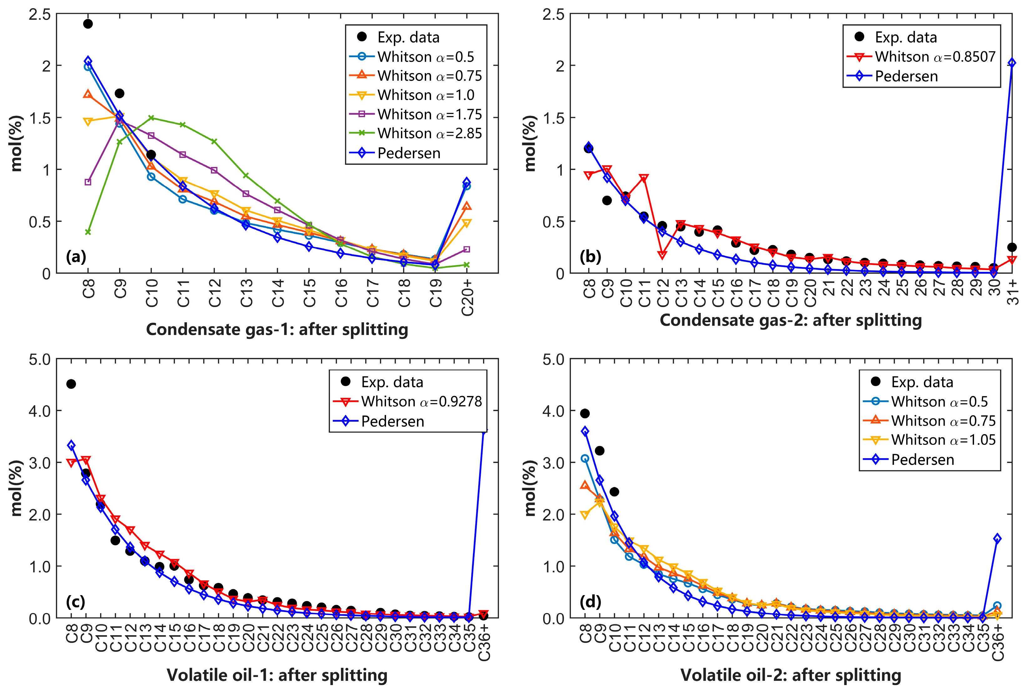
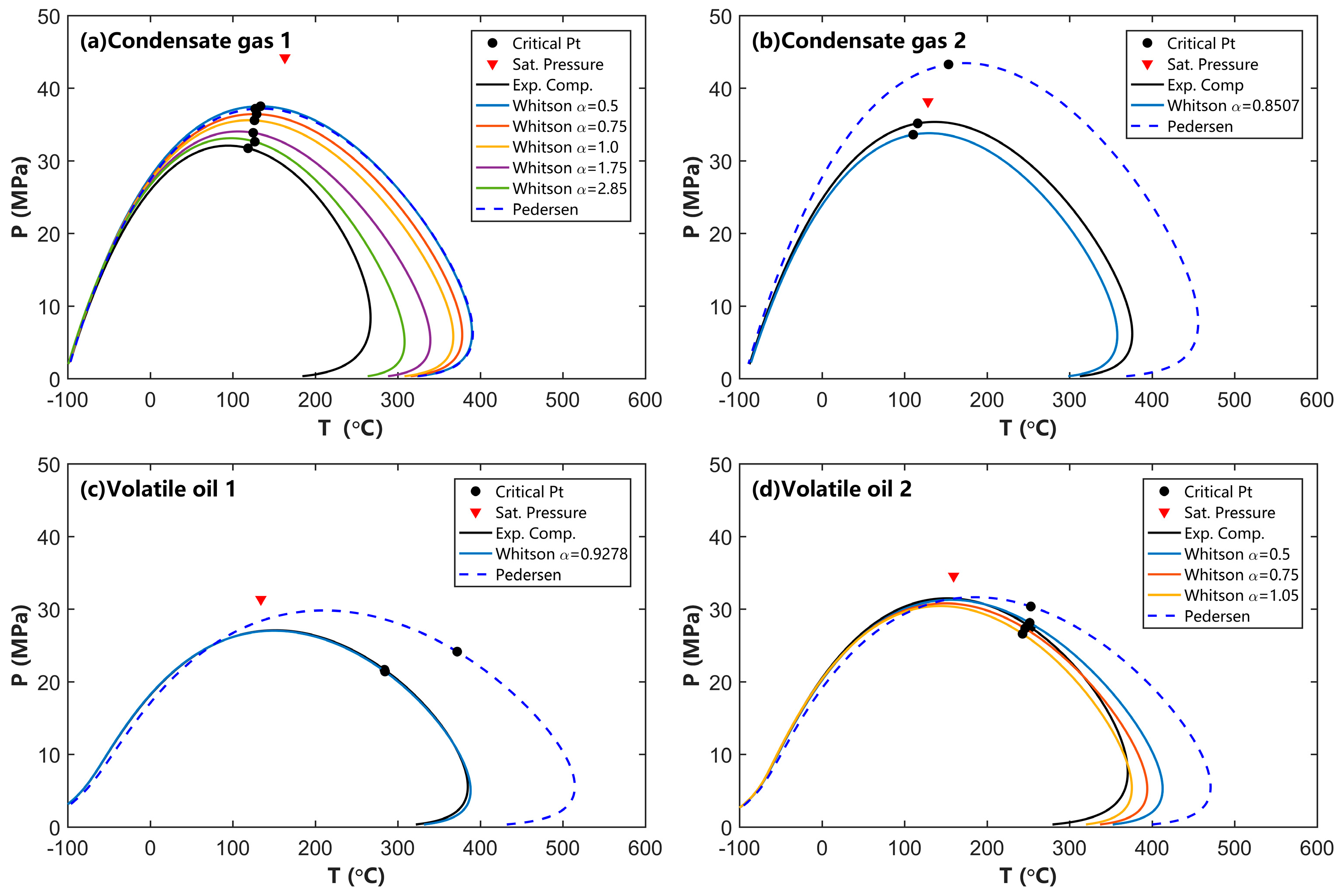
4.1. Effects of C7+ Splitting and SCN Group Distribution on the Phase Behavior Calculation

First, we consider the splitting of heptane plus components using the Pedersen and the Whitson methods. The comparison results between the calculated SCN distribution patterns and the experimental data are shown in Figure 4. This figure illustrates that the SCN distribution patterns obtained from the two different splitting methods exhibit significant differences after splitting. In Figure 4a, due to the lack of detailed component data for the condensate gas-1 sample, it can be observed that the distribution pattern provided by the Pedersen method is the closest to the experimental data (C₈–C₁₀) in terms of component distribution. However, when using the Whitson method to calculate the component distribution, the impact of different α values on the distribution results is substantial. When α = 0.5, the distribution pattern calculated by the Whitson method is almost identical to that obtained by the Pedersen method. As the α value increases from 0.5, the deviation between the results obtained by the Whitson method and those from the Pedersen method gradually increases.

Figure 4b corresponds to condensate gas-2 and shows that the mole fraction results calculated using the Pedersen method are significantly lower than the gas chromatography experimental data for components above C13, leading to a noticeable increase in the final C36+ components. In contrast, the Whitson method exhibits strong oscillations in the distribution of C11 and C12 components, but the components above C13 show a high degree of agreement with the experimental data. This pattern is also observed in volatile oil-1 (Figure 4c) and volatile oil-2 (Figure 4d).

There are significant differences between the Whitson method and the Pedersen method when splitting the C₁₁₊ group into components from C₁₁ to C₃₆₊ (Figure 4d). Specifically, the Pedersen method overestimates the mole fraction of the C₃₆₊ component when breaking down the C₁₁₊ component into C₁₁ through C₃₆₊. This leads to an overall smaller mole fraction for the C₁₁ to C₃₅ components compared to the results predicted by the Whitson method. In contrast, the Whitson method can achieve a more reasonable distribution of components (i.e., C₁₁ to C₃₆₊) by adjusting the α parameter.

By using the component distributions from Figure 4 to calculate the fluid phase diagrams, further observations were made in Figure 5. For condensate gas-1, due to the lack of experimental distribution information for heavy components, the phase diagram calculated directly using the experimental data shows a significant deviation from the actual reservoir saturation pressure (Figure 5a). When the component distribution is reconstructed using the Pedersen or Whitson splitting methods, the resulting phase envelope shows an improved match with the experimental saturation pressure. Additionally, the results from the Pedersen method and the Whitson method with α = 0.5 show the best agreement.

Condensate gas-2 and volatile oil-1 have detailed experimental heavy component distributions; when using Whitson’s method for these kinds of fluids, the α value is first calculated based on the experimental data using Equations (15)–(17). Then, the component distribution was calculated using this α value. Figure 5b,c shows that the fluid phase envelope calculated from the component distributions obtained from the Whitson method is highly consistent with those obtained from the experimental data. In contrast, the phase envelopes calculated using the Pedersen method show a wider gas–liquid two-phase region in temperature scale compared to the results from the Whitson method, highlighting the differences in phase diagram calculations between the two methods.

In Figure 5b, when using the experimental composition (solid black curve) and the distribution of the components estimated from the Whitson method (solid blue curve) to calculate the phase envelope, the fluid is identified as condensate gas because the critical temperature of the reservoir fluid is lower than the reservoir temperature. However, when using components distribution estimated from the Pedersen method to calculate the phase envelope (dashed blue curve), the reservoir fluid is identified as a volatile oil because the critical temperature on the dashed blue curve is higher than the reservoir temperature (Figure 5b). This observation indicates that different methods (i.e., Whitson or Pedersen) for predicting component distribution can lead to entirely different results in the classification of oil and gas reservoirs.

In Figure 5c, the reservoir saturation pressure calculated using Pedersen’s method (blue dashed curve) is closer to the experimental saturation pressure than that of Whitson’s method (blue curve). In Figure 5d, the saturation pressures obtained from both component distributions (i.e., Whitson and Pedersen) agree well; however, the phase envelope generated from the composition predicted by Pedersen’s method extends its two-phase region into a higher temperature range (Figure 5c,d). All these observations show that component distribution has a significant influence on the phase behavior of both volatile oil and condensate gas.

Figure 4 and Figure 5 illustrate that the fluid compositions obtained using different component splitting methods have a very significant impact on the phase behavior of reservoir fluids. The Pedersen method [9,10,11] typically results in fluids with a wider gas–liquid two-phase region and a higher critical temperature. In contrast, the Whitson method [12,13], when an appropriate α value is chosen, can reproduce the phase diagram of the experimental fluid composition as closely as possible. In the subsequent discussions of this paper, for condensate gas-1 and volatile oil-2, the α value for the Whitson method is set to 0.5. For condensate gas-2 and volatile oil-1, the α values for the Whitson method are 0.8507 and 0.9278, respectively.

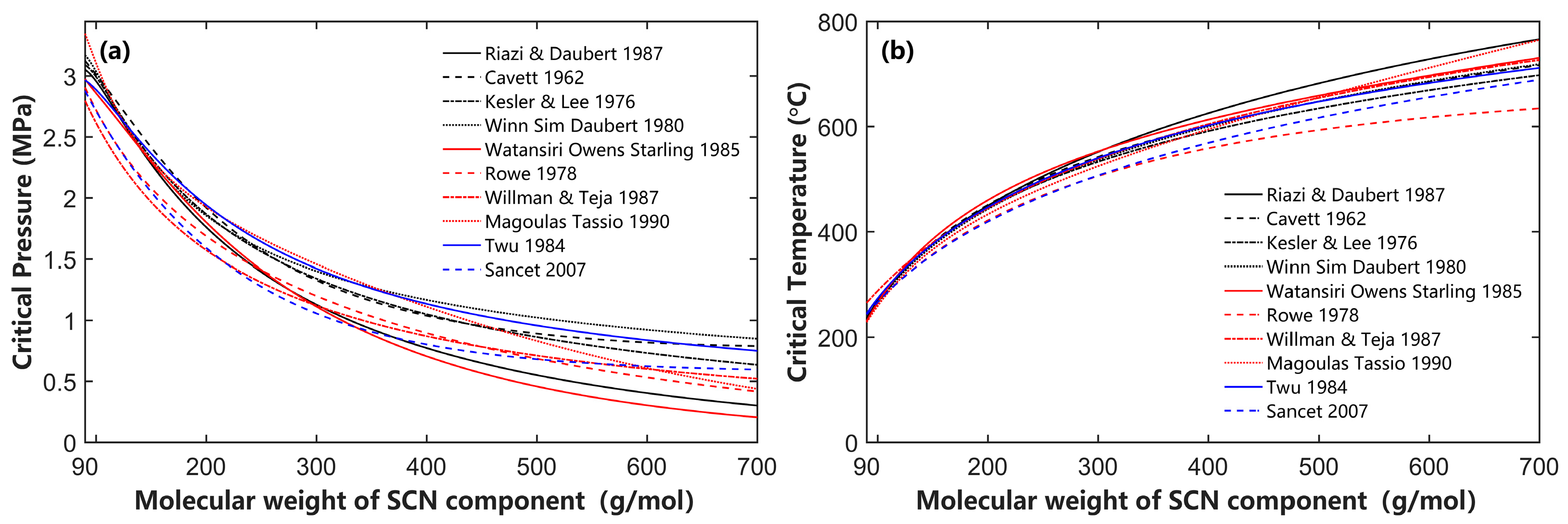
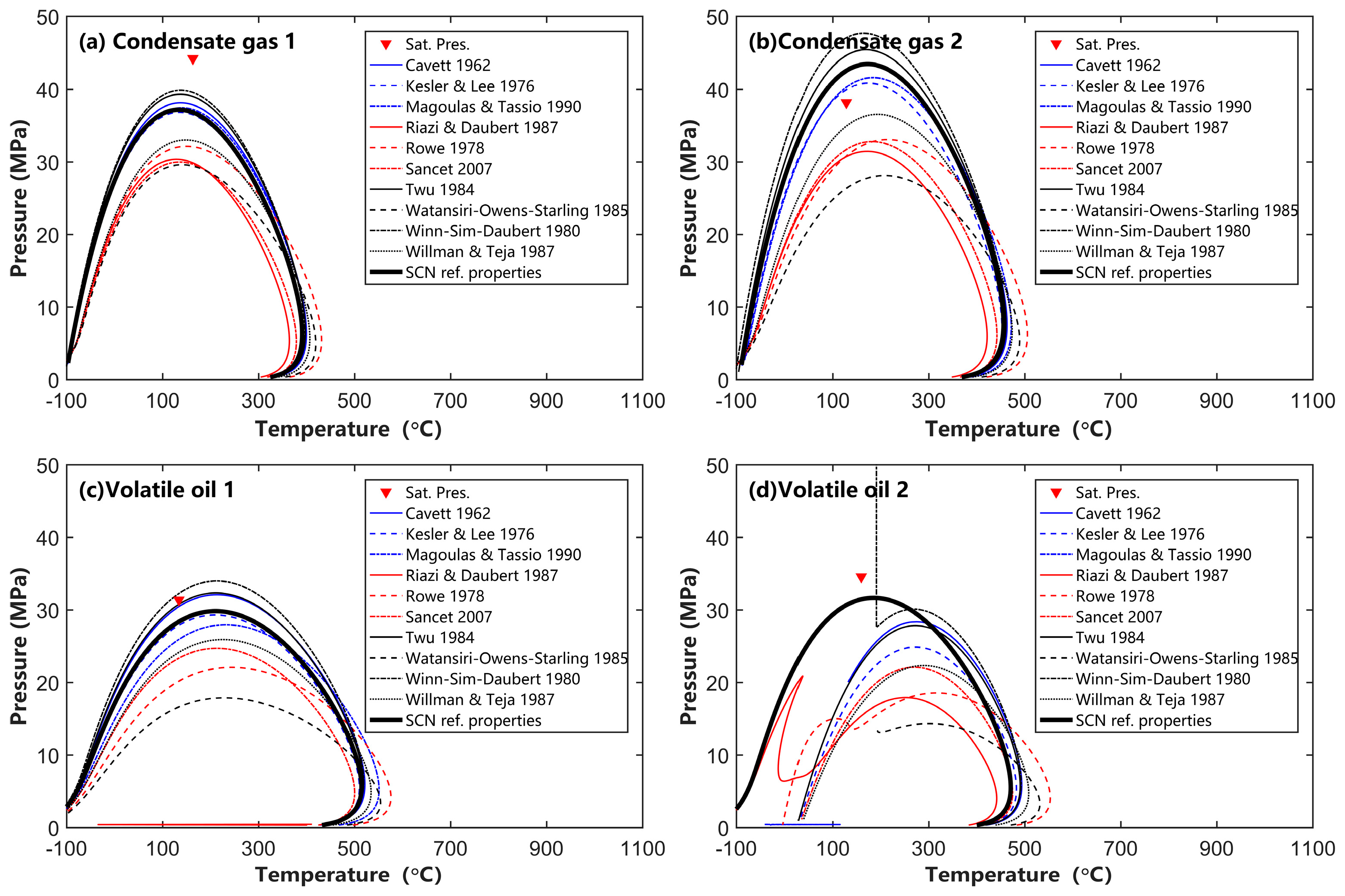
4.2. Effects of SCN Group Characterization on Phase Behavior Calculation

In the calculations for Figure 5, the EOS parameters ($P_{ci}$, $T_{ci}$, ${\omega }_i$) for each fluid’s (see Table A1) SCN components are required. These parameters, referred to as ‘SCN reference properties’, are taken from the literature (Whitson [28], Chapter 5, Table 5.2). Additionally, the literature provides various empirical formulas for estimating these SCN EOS parameters. The results obtained using different methods can also impact the calculation of reservoir fluid phase behavior and PVT properties.

Since these methods (Table 2, Figure 6 and Figure 7) for calculating EOS properties primarily rely on empirical formulas and these empirical formulas were fitted using experimental data from crude oils from different regions worldwide, the obtained EOS parameters among these methods exhibit differences. This discrepancy increases with increasing molecular weight. Therefore, the calibration and calculation of single carbon number (SCN) EOS parameters also significantly impact the calculation results of reservoir fluid phase behavior.

Figure 8 and Figure 9 show the differences in the phase diagrams of four fluids (see Appendix A Table A1) obtained after splitting using the Pedersen and Whitson methods, respectively, followed by the calculation of SCN EOS parameters using various methods listed in Table 2.

In Figure 8, all fluids are first split using the Pedersen method. Then, the EOS parameters are estimated using different methods, and the phase diagrams are calculated using the Michelsen saturation pressure curve tracing algorithm [27,29]. The EOS parameter estimation methods provided by Riazi and Daubert [17], Rowe [20], Sancet [24], Watansiri–Owens–Starling [19], and Willman and Teja [21] tend to underestimate the saturation pressure of reservoir fluids, resulting in a smaller gas–liquid two-phase region in the P-T phase diagram compared to the results calculated using SCN reference properties. On the other hand, the SCN EOS parameter estimation methods proposed by Cavett [16], Kesler and Lee [16], and Magoulas and Tassio [22] yield phase diagrams that are closer to those calculated using SCN reference properties. Compared to the phase diagrams calculated using SCN reference properties [28], the methods by Winn–Sim–Daubert [18] and Twu [23] tend to slightly overestimate the saturation pressure of reservoir fluids, causing the gas–liquid two-phase region to extend slightly into the higher-pressure area.

Figure 8 shows that the SCN group EOS parameter calculation methods provided by Riazi and Daubert [17], Rowe [20], Sancet [24], Watansiri–Owens–Starling [19], and Willman and Teja [16] are generally not applicable for describing the phase behavior of condensate gas and volatile oil. Additionally, both Figure 8c and Figure 9c show that the Riazi and Daubert methods [17] fail when computing phase envelopes for these strongly volatile reservoir fluids. By comparing Figure 8 and Figure 9, it can also be seen that when using the Whitson splitting method (Figure 9), the obtained phase envelopes show a shrinkage of the gas–liquid two-phase region on the phase envelope when compared to that from the Pedersen method (Figure 8).

For condensate gas 2, when the component distribution is obtained using the Pedersen method, the phase envelope with the lowest saturation pressure in Figure 8b is obtained using the SCN group EOS parameters calibrated by the Watansiri–Owens–Starling method [19], with a maximum pressure of approximately 28.15 MPa. Meanwhile, the phase envelope with the highest saturation pressure in Figure 8b is obtained using the EOS parameters calculated by the Winn–Sim–Daubert method [18], with a maximum pressure of approximately 47.73 MPa. For the same fluid, the maximum pressure of the phase diagrams obtained by these two EOS parameter calculation methods [18,19] differs by 19.58 MPa, a discrepancy that is difficult to improve during the later EOS parameter fitting process. Similarly, for condensate gas 2, when the component distribution is obtained using the Whitson method, the maximum pressure difference of the phase envelopes is reduced from 19.58 MPa in Figure 8b to 8.29 MPa in Figure 9b.

Figure 8d and Figure 9c,d show that some EOS parameter estimation methods cannot reliably calculate the phase envelope of volatile oil. For example, in Figure 8d, the saturation pressure curves obtained using the EOS parameters from the Riazi and Daubert method [17] and the Rowe method [20] differ significantly from the typical phase behavior of reservoir fluids. In Figure 9c, the EOS parameters obtained using the Riazi and Daubert method [17] result in a phase envelope that, when calculated using Michelsen’s saturation pressure curve tracking algorithm [29], only produces a slanted line on the low-temperature side (in the −100 °C to −70 °C range). When using the EOS parameters obtained from the Watansiri–Owens–Starling method [19] (Figure 9c), the Winn–Sim–Daubert method [18] (Figure 8d), the Rowe method [20] (Figure 8d), the Riazi and Daubert method [17] (Figure 8d), and the Willman and Teja method [21] (Figure 9d) to calculate the phase diagram, anomalies appear near the maximum pressure point of the phase envelope, with the phase envelope suddenly extending toward the high-pressure side or phase envelope calculation fails at the low-temperature side. Additionally, there are instances where the phase diagram calculation fails to converge (the Watansiri–Owens–Starling method [19] in Figure 8d and Figure 9d, and the Rowe method [20] in Figure 9d).

The abnormal phase envelope results mentioned above indicate that the corresponding SCN group EOS parameter estimation methods (i.e., Watansiri–Owens–Starling, Rowe, Riazi and Daubert, Willman and Teja, and Winn–Sim–Daubert methods) in Table 2 are not suitable for volatile oil. Special attention is needed during practical use, and further validation with PVT experimental data is required.

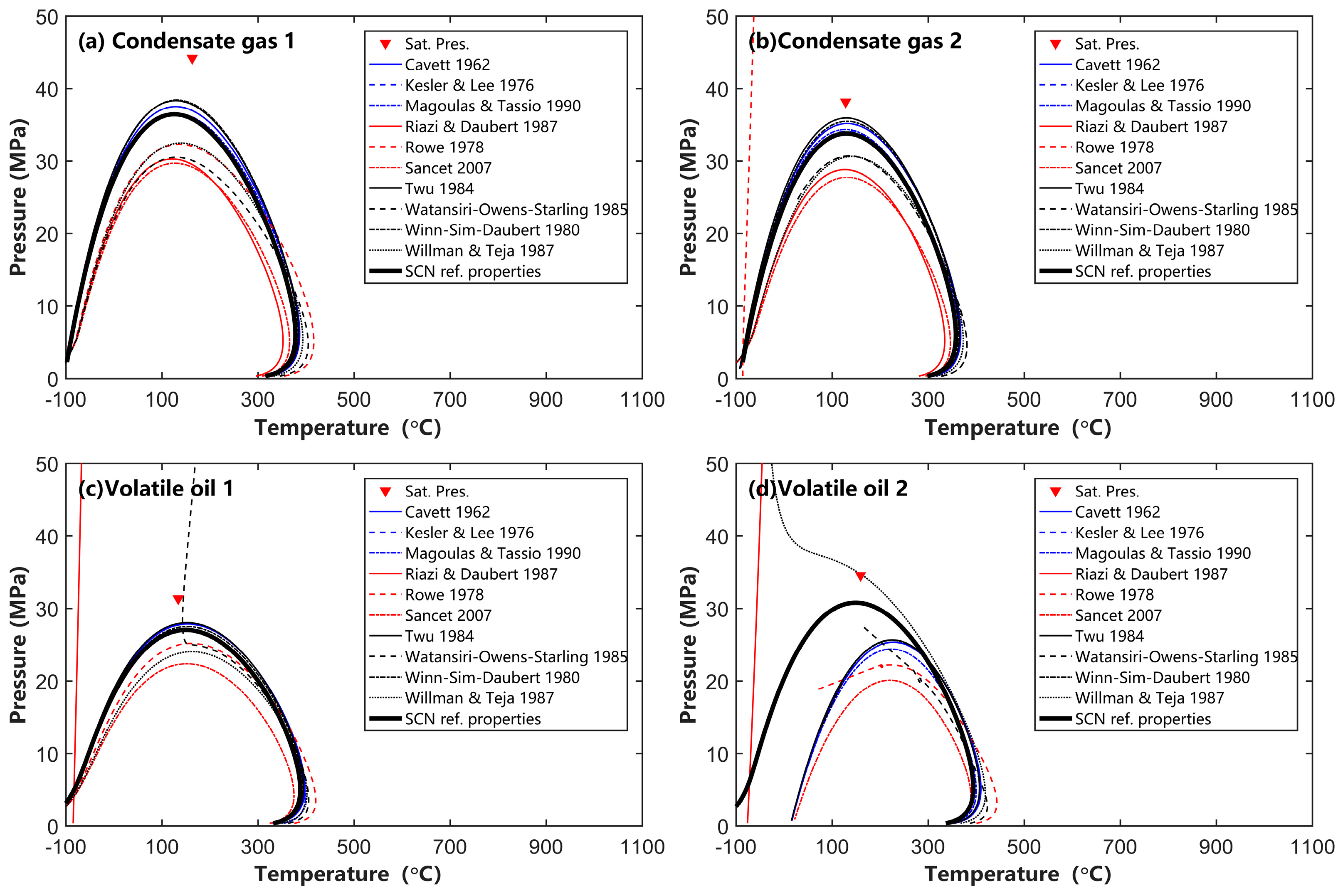
4.3. Effects of the SCN Group Lumping Scheme on the Phase Behavior Calculation

Through the comparative analysis mentioned above, when studying the effect of single carbon number (SCN) component lumping methods on phase behavior calculation results, the fluid composition obtained from the Whitson splitting method combined with the SCN reference EOS properties was selected for calculation. The specific SCN component lumping strategy is shown in Figure 10. For each reservoir fluid, calculations were compared using both the Whitson lumping method [12,13] and the Newley and Merrill lumping method [25]. The Pedersen component splitting method and other SCN group EOS parameter estimation methods listed in Table 2 also yield similar conclusions.

After component lumping based on the strategy outlined in Figure 10, each fluid is represented between four and five pseudo-components for all C7+ components, significantly reducing the computational load for phase behavior and compositional reservoir simulations. The results (Figure 11) indicate that the differences between the two lumping schemes selected in this study are minimal. Except for volatile oil 2 (Figure 11d), after component lumping, the phase envelopes and critical points of the fluids can be accurately reproduced without bias compared to the original component distribution without lumping. Both the Whitson and Newley–Merrill lumping methods demonstrate satisfactory performance. Therefore, the selection between these two lumping methods has a negligible impact on the phase behavior calculations of condensate gas and volatile oil.

In this study, we used Michelsen’s saturation pressure curve tracing algorithm for computing the phase envelope [27,29]. This algorithm, while relatively complex in its calculation process, is fast and exhibits good convergence given that the EOS parameters are well-prepared. The comparison of the phase diagram calculations reveals that component splitting and SCN group EOS parameter estimation significantly impact the phase behavior of reservoir fluids, whereas the effect of component lumping is minimal. This study does not address the tuning of EOS parameters before and after component lumping; this topic will be discussed separately in future work.

5. Conclusions

(1)

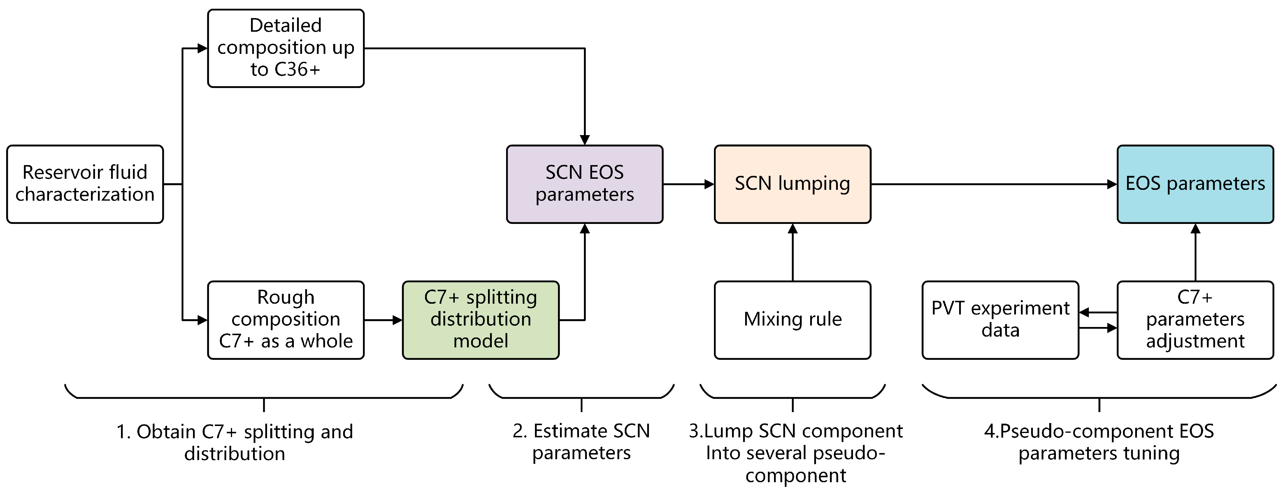
A workflow including three main steps (1. determine distribution pattern; 2. determine EOS parameters for SCN group; and 3. lump individual SCN group) for the characterization of EOS parameters for reservoir fluids was proposed (Figure 1);

(2)

The choice of component splitting and SCN group EOS parameter calculation methods significantly impact the phase behavior calculations, whereas the SCN group lumping methods have a minimal impact on the phase behavior calculation results;

(3)

The SCN group distribution obtained using the Whitson splitting method is closer to the experimental data compared to Pedersen’s splitting method. Additionally, for condensate gas and volatile oil, we recommended that the parameter α in the Whitson component distribution model ranges between 0.5 and 1.0 for the most accurate representation of component distribution for these reservoir fluids;

(4)

The EOS parameter calculation methods proposed by Cavett, Kesler and Lee, Twu, and Magoulas and Tassios, when combined with the Whitson component distribution, can reliably calculate phase behavior for condensate gas and volatile oil. However, other EOS parameter calculation methods are not recommended for engineering calculations of condensate gas and volatile oil reservoirs;

(5)

In terms of component lumping methods, the Whitson method and the Newley and Merrill method exhibit similar performance.

References

1. Zhang, N.; Ya, Q. Evaluation of the phase behavior of CO2 injection in condensate gas wells considering formation water. Xinjiang Oil Gas 2013, 9, 76–80. [Google Scholar]
2. Sun, Y.; Meng, Y.; Lian, Z.; Tang, Y.; Chen, K.Z. Influence of the splitting schemes on the heavy fractions characterization procedure. Complex Hydrocarb. Reserv. 2009, 2, 39–43. [Google Scholar]
3. Zachopoulos, F.N.; Kokkinos, N.C. Detection methodologies on oil and gas kick: A systematic review. Int. J. Oil Gas Coal Technol. 2023, 33, 1–19. [Google Scholar] [CrossRef]
4. Zachopoulos, F.N.; Kokkinos, N.C. Mathematical modeling of oil and gas kick during drilling operations. In Proceedings of the 11th International Conference on Mathematical Modeling in Physical Sciences, Belgrade, Serbia, 5–8 September 2022. [Google Scholar]
5. Kokkinos, N.C. Modeling and simulation of biphasic catalytic hydrogenation of a hydroformylated fuel. Int. J. Hydrogen Energy 2021, 46, 19731–19736. [Google Scholar] [CrossRef]
6. Peng, D.; Robinson, D.B. A New Two-Constant Equation of State. Ind. Eng. Chem. Fundam. 1976, 15, 59–64. [Google Scholar] [CrossRef]
7. Soave, G. Equilibrium constants from a modified Redlich-Kwong equation of state. Chem. Eng. Sci. 1972, 27, 1197–1203. [Google Scholar] [CrossRef]
8. Liu, C.; Zhang, M.; Mei, H.; Liu, Y. Phase behavior of condensate gas reservoir fluids and influencing factors. Xinjiang Oil Gas 2007, 3, 62–66. [Google Scholar]
9. Pedersen, K.S.; Thomassen, P.; Fredenslund, A. SRK-EOS calculation for crude oils. Fluid Phase Equilibria 1983, 14, 209–218. [Google Scholar] [CrossRef]
10. Pedersen, K.S.; Thomassen, P.; Fredenslund, A. Thermodynamics of petroleum mixtures containing heavy hydrocarbons. 1. Phase envelope calculations by use of the Soave-Redlich-Kwong equation of state. Ind. Eng. Chem. Process Des. Dev. 1984, 23, 163–170. [Google Scholar] [CrossRef]
11. Pedersen, K.S.; Christensen, P.L. Phase Behavior of Petroleum Reservoir Fluids; CRC Press: Boca Raton, FL, USA, 2007. [Google Scholar]
12. Whitson, C.H. Characterizing hydrocarbon plus fractions. SPE J. 1983, 23, 683–694. [Google Scholar] [CrossRef]
13. Whitson, C.H. Effect of C7+ properties on equation-of-state predictions. SPE J. 1984, 24, 685–696. [Google Scholar] [CrossRef]
14. Duan, J.; Wang, W.; Liu, H.; Gong, J. Modeling the characterization of the plus fractions by using continuous distribution function. Fluid Phase Equilibria 2013, 35, 1–10. [Google Scholar] [CrossRef]
15. Foroughi, S.; Khoozan, D.; Jamshidi, S. Optimal distribution function determination for plus fraction splitting. Can. J. Chem. Eng. 2019, 97, 2752–2764. [Google Scholar] [CrossRef]
16. Ahmed, T. Equations of State and PVT Analysis Applications for Improved Reservoir Modeling; Gulf Professional Publishing: Houston, TX, USA, 2016. [Google Scholar]
17. Riazi, M.R.; Daubert, T.E. Characterization parameters for petroleum fractions. Ind. Eng. Chem. Res. 1987, 26, 755–759. [Google Scholar] [CrossRef]
18. Sim, W.J.; Daubert, T.E. Prediction of vapor-liquid equilibria of undefined mixtures. Ind. Eng. Chem. Process Des. Dev. 1980, 19, 386–393. [Google Scholar] [CrossRef]
19. Watansiri, S.; Owens, V.H.; Starling, K.E. Correlations for estimating critical constants, acentric factor, and dipole moment for undefined coal-fluid fractions. Ind. Eng. Chem. Process Des. Dev. 1985, 24, 294–296. [Google Scholar] [CrossRef]
20. Rowe, A.M. Internally consistent correlations for predicting phase compositions for use in reservoir composition simulations. In Proceedings of the SPE Annual Technical Conference and Exhibition, Houston, TX, USA, 1–3 October 1978. [Google Scholar]
21. Willman, B.; Teja, A.S. Prediction of dew points of semicontinuous natural gas and petroleum mixtures. 1. Characterization by use of an effective carbon number and ideal solution predictions. Ind. Eng. Chem. Res. 1987, 26, 948–952. [Google Scholar] [CrossRef]
22. Magoulas, K.; Tassios, D. Thermophysical properties of n-Alkanes from C1 to C20 and their prediction for higher ones. Fluid Phase Equilibria 1990, 56, 119–140. [Google Scholar] [CrossRef]
23. Twu, C.H. An internally consistent correlation for predicting the critical properties and molecular weights of petroleum and coal-tar liquids. Fluid Phase Equilibria 1984, 16, 137–150. [Google Scholar] [CrossRef]
24. Sancet, G.F. Heavy fraction C7+ characterization for PR-EOS. In Proceedings of the SPE Annual Technical Conference and Exhibition, Anaheim, CA, USA, 11–14 November 2007. [Google Scholar]
25. Newley, T.M.J.; Merrill, R.C., Jr. Pseudocomponent selection for compositional simulation. SPE Reserv. Eng. 1991, 6, 490–496, SPE-19638-PA. [Google Scholar] [CrossRef]
26. Hong, K.C. Lumped-component characterization of crude oils for compositional simulation. In Proceedings of the SPE Enhanced Oil Recovery Symposium, Tulsa, OK, USA, 4–7 April 1982. SPE-10691-MS. [Google Scholar]
27. Zhao, H.; Song, C.; Zhang, H.; Di, C.; Tian, Z. Improved fluid characterization and phase behavior approaches for gas flooding and application on Tahe light crude oil system. J. Pet. Sci. Eng. 2022, 208 Pt D, 109653. [Google Scholar] [CrossRef]
28. Whitson, C.H.; Brulé, M.R. Phase Behavior, SPE Monograph Volume 20; Society of Petroleum Engineers: Houston, TX, USA, 2000. [Google Scholar]
29. Michelsen, M.L. Calculation of phase envelopes and critical points for multicomponent mixtures. Fluid Phase Equilibria 1980, 4, 1–10. [Google Scholar] [CrossRef]
Figure 1. Overall workflow of heptane plus characterization and EOS parameters determination.
Processes 12 02066 g001
Figure 2. Illustration of the component lumping method proposed by Newley and Merrill.
Processes 12 02066 g002
Figure 3. Heptane plus component characterization methods [16,17,18,19,20,21,22,23,24] are considered in this study.
Processes 12 02066 g003
Figure 4. Comparison of the calculation results from different C7+ splitting methods. (a) condensate gas sample with experimental composition up to C11+; (b) condensate gas sample with detailed experimental composition distribution up to C36+; (c) volatile oil sample with detailed experimental composition distribution up to C36+; (d) volatile oil sample with experimental composition up to C11+.
Processes 12 02066 g004
Figure 5. Effects of the C7+ splitting method on the phase behavior of gas condensate and volatile oil.
Processes 12 02066 g005
Figure 6. The differences in EOS parameters ((a) critical pressure and (b) critical temperature) of the SCN group are calculated from various methods [16,17,18,19,20,21,22,23,24].
Processes 12 02066 g006
Figure 7. The differences in the Pitzer acentric parameter of the SCN group are calculated from various methods [16,22,23].
Processes 12 02066 g007
Figure 8. Effects of various SCN EOS parameters estimated from different sources [16,17,18,19,20,21,22,23,24] on phase behavior of gas condensate and volatile oil (SCN group distribution was obtained from Pedersen’s model, and SCN reference properties were taken from Table 5.2 in the literature [28]).
Processes 12 02066 g008
Figure 9. Effects of various SCN EOS parameters estimated from different sources [16,17,18,19,20,21,22,23,24] on the phase behavior of gas condensate and volatile oil (SCN group distribution was obtained from Whitson’s model, for condensate gas-1, condensate gas-2, volatile oil-1, and volatile oil-2, α equals 0.75, 0.8507, 0.9278, and 0.75, respectively).
Processes 12 02066 g009
Figure 10. Heptane plus SCN group lumping scheme (N and M represent the lumping methods proposed by Newley–Merrill [25]).
Processes 12 02066 g010
Figure 11. Effects of the heptane plus SCN group lumping scheme on phase behavior calculation (“Whitson splitting unlumped” means no lumping was applied; the detailed lumping scheme of Newley and Merrill method as well as Whitson’s method refers to Figure 10).
Processes 12 02066 g011