Improving the Feedforward Component for Recent Variants of Predictive Functional Control

Abstract

A recent study demonstrated that the use of feedforward information with conventional Predictive Functional Control (PFC) leads to unexpected inconsistencies, with subsequent negative impacts on tuning and behaviour. A proposal was made to define the coincident point differently and shown to reduce the lag in the closed-loop PFC responses and applied to some systems with benign dynamics. Other recent work has looked at parameterisations of the future input to deal with challenging open-loop dynamics and significantly extended the range of problems for which PFC can be effective. This paper combines the two concepts, and thus proposes an algorithm that has both more effective and simple tuning than original PFC as well as being applicable to a range of challenging dynamics.

1. Introduction

This paper takes as its context Model Predictive Control (MPC) [1,2,3,4,5,6,7,8]. There have been an enormous number of papers published in this area showing how MPC algorithms can be tailored to specific objectives and requirements (e.g., [9,10]), but in the main these approaches focus on algorithms that require substantial computational power. However, the particular focus of this paper is efficient or indeed highly efficient MPC, thus predictive algorithms for which the coding is simple and indeed of similar complexity and cost to PID. There are very few alternatives in the literature meeting this remit because it means that any systematic constraint handling cannot involve an online optimisation, but rather a small number of simple checks which can be coded simply and transparently.

Of the few very efficient MPC approaches in the literature, that is those with comparable complexity to PID, it makes sense to summarise a few before moving on with the contribution of this paper. The original reference governor approaches modified the performance index to focus more on a constraint handling algorithm which required the simplest change to the system target [11]. These algorithms were simple to implement but the optimisation objective was crude and thus more recent variants have attempted to capture the performance more carefully, but unsurprisingly, with the consequence that these are computationally much more demanding. More recently the development of parametric approaches [9,12] has a similar philosophy, that is to reduce and simplify the online implementation of constraint handling. However, while the philosophy is appealing, in most cases parametric approaches are actually hugely complicated to design and also require substantial online computation. By comparison, one approach which has had significant commercial success and can genuinely claim to be very simple to code is the Predictive Functional Control (PFC) approach [13,14,15,16]. This is very simple and cheap to implement and thus popular in industry where effective [13,17,18,19], but unsurprisingly therefore, does have some weaknesses such as: (i) weak stability and feasibility results [20] and (ii) the tuning is not always as effective nor as intuitive as desired [21].

1.1. Review of Recent Developments in PFC

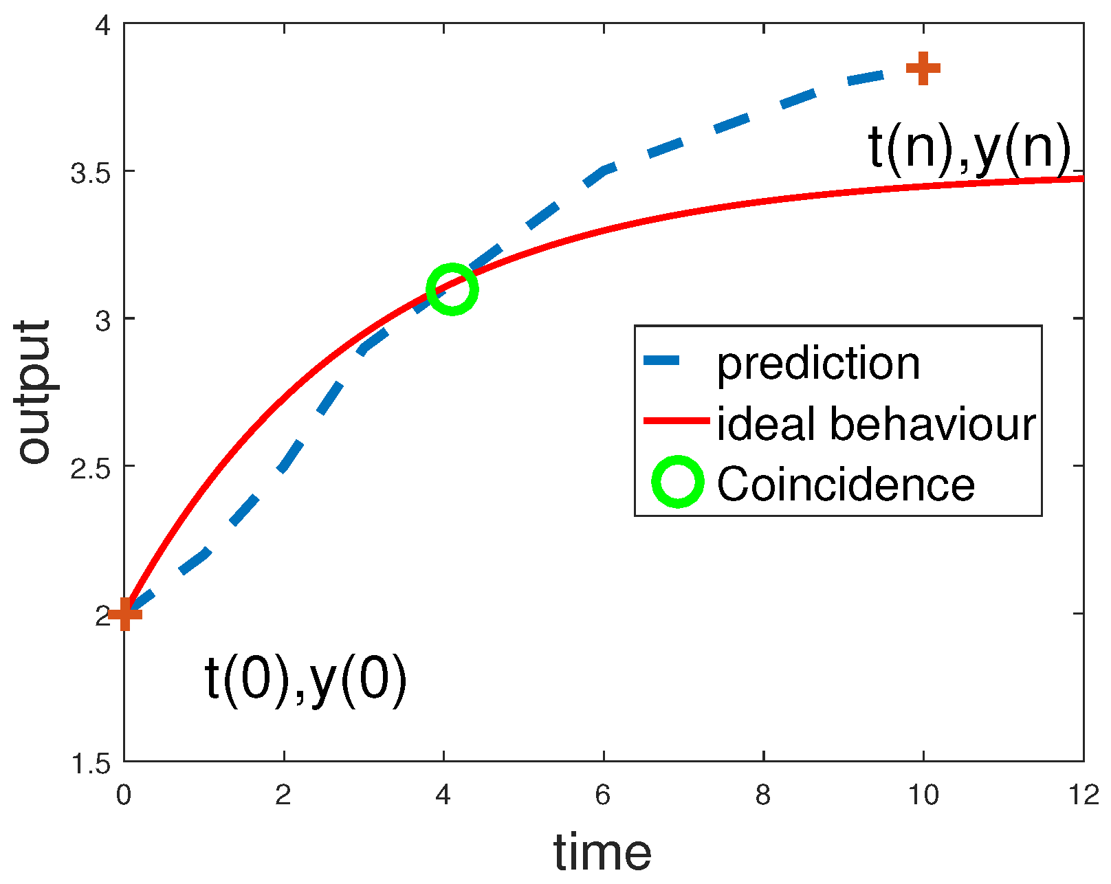
The basic concept underpinning PFC is that we want the system output to move smoothly towards the target, somewhat akin to a 1st order response, and indeed the main design parameter is the associated or desired closed-loop time constant. Hence, much like a human might do, we estimate the future system input which will drive the system prediction to duplicate the desired/ideal 1st order behaviour, but critically for computational simplicity, only at a single point in time (the coincidence point) as shown in Figure 1.

This simplicity is what causes weaknesses and two core weaknesses have been exposed and tackled in the more recent literature.

• The predictions (for constant targets) are based on the assumption that the future input will also be constant, thus embedding open-loop behaviours into the predictions. Where open-loop behaviours are far from ideal, such an embedding can be counter productive [20,21].
• The coincidence point shown in Figure 1 is constructed using the distance between the current output and the target, but where the system dynamics have significant lag, this definition introduces inconsistency from one sample to the next [22], with a corresponding loss in performance.

Hence, the most popular recent thrust in the research into PFC has looked at how to modify the input parameterisation within the predictions (e.g., [16,23,24]) and these proposals do indeed, often outperform the conventional PFC approach. More recent work with the same underlying ethos, has considered the extent to which some pre-stabilisation or pre-conditioning can help, in essence, add a simple inner loop based on classical control such as PID [25,26]. By ensuring the nominal dynamics are better in the first place, a conventional PFC algorithm is able to operate much more effectively.

A much more recent proposal is to investigate the concept of coincidence which is the core of PFC and question whether the coincidence point itself has been defined effectively? Some novel analysis [22] showed that for many systems, the coincidence point itself may not be an effective start point for a predictive control design, because the conventional definition was introducing inconsistent decision making. In fact, closer analysis showed that it was not the concept of coincidence that was flawed, but rather, how the point was being defined. A very small modification to this definition allowed significant improvements in tuning efficacy.

1.2. Research Gaps in PFC and Paper Contribution

There are still some obvious research paths that have not been studied and these form the main basis of the contributions in this paper.

• Reparameterising the predicted input [25,26] seems to make good sense and helps hugely where the open-loop dynamics are anything other than a well damped system with little lag. However, on its own, it does not solve the poor tuning efficacy.
• Re-defining the coincidence point [22] improves the tuning efficacy for systems with over-damped dynamics, but on its own, may not help with difficult dynamics.

Consequently, it would seem logical to combine the two concepts above and thus consider how the modified coincident point definition in combination with altered prediction parameterisations, will give an algorithm that is: (i) computationally very simple to code and implement and (ii) intuitive and effective to tune, even for challenging open-loop dynamics.

This paper will begin in Section 2 by introducing the standard background on PFC, the coincident point and discuss concisely some of the relevant recent proposals in the literature. Section 3 will present the main contribution, which is the combination of results from [22] with those from earlier proposals [25,26]. Section 4 will give a number of numerical case studies exploring tuning efficacy, behaviours, sensitivity and pole positions for both the proposed algorithm and more recent alternative algorithms. The paper then finishes with some conclusions.

2. Background on PFC

This section reviews existing concepts, ideas and developments in PFC which are an essential background for the proposals given later in the paper. A more detailed summary and review is available in the recent Processes paper [27] and indeed other references. The most important concepts are: (i) the conventional PFC algorithm; (ii) modification of the coincident point definition/feedforward and (iii) alternative parameterisations of the input predictions to improve tuning efficacy and stability.

2.1. The Independent Model

For clarity, the two different approaches of [22] and conventional PFC [13] are summarised here with a focus on core concepts rather than the technical details which are already widely published. For simplicity we assume a process $G_p\left(z\right)=b_p\left(z\right)/a_p\left(z\right)$ and model $G_m\left(z\right)=b_m\left(z\right)/a_m\left(z\right)$ respectively of the form:

$$a_p\left(z\right)y_p\left(z\right)=b_p\left(z\right)u\left(z\right)+\eta \left(z\right);a\left(z\right)y_m\left(z\right)=b\left(z\right)u\left(z\right)$$

(1)

where z is the normal Z-transform operator for discrete systems, $y_p\left(z\right),y_m\left(z\right),u\left(z\right)$ are the process and system outputs and input respectively. Also define the offset between the process and model outputs are sample k as $d_k=y_{p,k}-y_{m,k}$. We assume that the process output $y_p$ (and thus also $d_k$) is measurable but $a_p,b_p$ and $\eta$ are unknown. Thus predictions are made using the model, and corrected for bias using $d_k$.

2.2. The Conventional PFC Algorithm

It is useful first to define the PFC control law in terms of concepts, before then showing how this can be expressed in mathematical form. The PFC control law is based on the concept that the distance between the current target $r_k$ and the predicted output should decrease monotonically, as shown in Figure 2 by the ideal curve. Thus if the distance at the current sample is $D_k$, then the desired distance n-steps ahead will be ${\lambda }^n{D}_k$ (note that $0<\lambda <1$ as in effect $\lambda$ is the desired closed loop pole). The corresponding control law given below is derived from this:

$$\left.\begin{array}{c}{D}_k=r_k-y_{p,k}\hfill \\ D_{k+n}={\lambda }^n{D}_k\hfill \\ D_{k+n}=r_k-E\left[y_{p,k+n|k}\right]\hfill \end{array}\right\}\Rightarrow r_k-E\left[y_{p,k+n|k}\right]={\lambda }^n(r_k-y_{p,k})$$

(2)

where $E\left[y_{p,k+n|k}\right]$ is the expected n-step ahead system prediction at sample time k, $\lambda$ is the desired closed-loop pole, r is the target, n is a coincidence horizon. The conventional PFC control law is based on enforcing (2) and is usually stated as follows:

$$E\left[y_{p,k+n|k}\right]=(1-{\lambda }^n)r_k+{\lambda }^n{y}_{p,k}=R_{k+n|k}$$

(3)

The notation $R_{k+n|k}$ is the implied target values for different n.

Remark 1.

We have not included details linked to non-zero dead-time systems to avoid unduly complicating the algebra, but this is straightforward and covered in the references.

2.3. Modifying the Use of Feedforward in PFC

The modified PFC control law proposed in [22] does not use output measurements in the definition of the target point, as this can cause the target $R_{k+n|k}$ to change somewhat erratically, that is, it can give inconsistent requirements from one sample to the next, especially with non-minimum phase systems. Instead, the target behaviour dependence on the set point was considered fixed and it is up to the control law to try and meet this. Nevertheless, as will be seen below, the target behaviour does move when disturbances are detected, as would be expected.

Ignoring disturbances for now, the modified PFC is given from:

$$E\left[y_{p,k+n|k}\right]=R_{k+n|k}$$

(4)

where critically, $R_{k+n|k}$ will be defined differently from (3), that is, a target trajectory based solely on a filtered version of the actual target $r_k$ and which is updated each sample as follows:

$$\begin{array}{ccc}\hfill R_{k+i|k}& =& [(1-\lambda ),(1-{\lambda }^2),(1-{\lambda }^3),\cdots ](r_k-r_{k-1})\hfill \\ & & +[R_{k+2|k-1},R_{k+3|k-1},R_{k+4|k-1},\cdots ]\hfill \end{array}$$

(5)

Critically, here the term $R_k$ is not affected by the actual system behaviour and thus, in the form of (5), is determined solely as a feedforward term. Readers will note that for the definition in (3) the target $R_{k+n|k}$ depends upon the current output measurement.

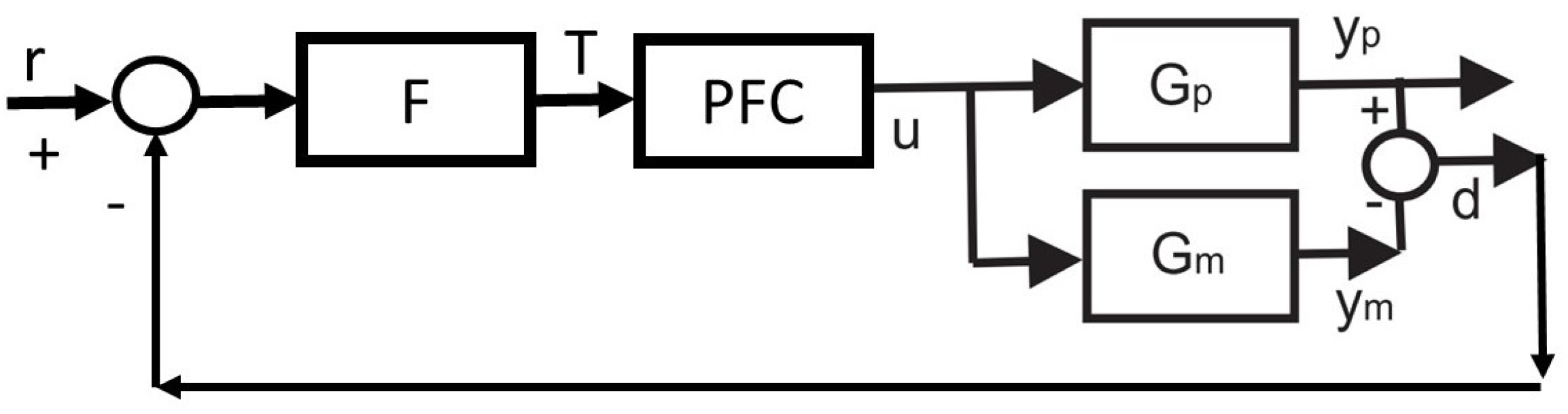
Remark 2.

An efficient realisation of (5) is given by the following transfer function representation:

$$T\left(z\right)=\left[1-\frac{(1-z^{-1}){\lambda }^n}{(1-\lambda z^{-1})}\right]r\left(z\right);T_k=R_{k+n|k}$$

(6)

Remark 3.

It is conventional in PFC to use an independent model for prediction so that one forms predictions $y_{m,k+i|k}$ based on a model, and then modify these for bias using the term:

$$d_k=y_{p,k}-y_{m,k}\Rightarrow E\left[y_{p,k+n|k}\right]=y_{m,k+n|k}+d_k$$

(7)

These terms impact on the target trajectory $R_{k+n}$ in an equivalent manner to (2) and (5), so that one can form a combined term:

$$T\left(z\right)=\underset{F\left(z\right)}{\underbrace{\left[1-\frac{(1-z^{-1}){\lambda }^n}{(1-\lambda z^{-1})}\right]}}(r\left(z\right)-d\left(z\right))$$

(8)

and control law (4) is replaced by:

$$y_{m,k+n|k}=T_k$$

(9)

Note the use of the independent model output in (9) as the disturbance and uncertainty effects are absorbed into $T_k$! As mentioned above, the dependence of $T_k$ on the target is not affected by system behaviour and depends solely on $r_k$. However, as $d_k$ depends on both the system and model, this term in $T_k$ must be updated every sample as the new $d_k$ is computed. A symbolic block diagram representation of (9) is shown in Figure 2, for now not including full details of how the PFC block works.

2.4. Conventional PFC Law with and without Feedforward Correction

In order to implement the control laws of (3) and (9) we need the independent model predictions [4,6]. Thus, it is known one can write:

$$y_{m,k+n|k}=H_n\underrightarrow{{\displaystyle u_k}}+P_n\underleftarrow{{\displaystyle u_{k-1}}}+Q_n\underleftarrow{{\displaystyle y_{m,k}}}$$

(10)

where matrices/vectors $H_n$, $P_n$, $Q_n$ depend on the model parameters and

$$\underrightarrow{{\displaystyle u_k}}=\left[\begin{array}{c}{u}_k\\ u_{k+1}\\ ⋮\\ u_{k+n-1}\end{array}\right]=\underset{L}{\underbrace{\left[\begin{array}{c}1\\ 1\\ ⋮\\ 1\end{array}\right]}}{u}_k;\underleftarrow{{\displaystyle u_{k-1}}}=\left[\begin{array}{c}{u}_{k-1}\\ u_{k-2}\\ ⋮\\ u_{k-n_b}\end{array}\right];\underleftarrow{{\displaystyle y_{m,k}}}=\left[\begin{array}{c}{y}_{m,k}\\ y_{m,k-1}\\ ⋮\\ y_{m,k-n_a}\end{array}\right]$$

(11)

for denominator/numerator with orders $n_a,n_b$ respectively and assuming future inputs are constant ($u_{k+i|k}=u_k$ for $i>0$).

The two control laws (e.g., [22]) can now be summarised.

The standard PFC law is determined by solving (3) for $u_k$ at every sample, thus is given from the following identity.

$$H_{n}L{u}_k+P_n\underleftarrow{{\displaystyle u_{k-1}}}+Q_n\underleftarrow{{\displaystyle y_{m,k}}}+d_k=(1-{\lambda }^n)r_k+{\lambda }^n{y}_{p,k}$$

(12)

The modified PFC law of (9) is determined by solving for $u_k$ at every sample the following identity.

$$H_{n}L{u}_k+P_n\underleftarrow{{\displaystyle u_{k-1}}}+Q_n\underleftarrow{{\displaystyle y_{m,k}}}=T_k$$

(13)

with $T_k$ defined by (8).

Remark 4.

The reader will note that the computational loads for both control laws are trivial and essentially the same. In fact, the main computational load is around the constraint handling aspects (e.g., [23]) which are not discussed here as not central to the core paper contribution.

2.5. Closed-Loop Pole Computations—Nominal Case

In order to assess the efficacy of tuning in the nominal case, it is necessary to express the PFC control law in z-transforms and derive the appropriate block diagram; these details are given next. For simplicity of analysis we use the nominal case and thus assume that $d_k=0,y_p=y_m$; clearly the poles will change for the uncertain case but not in the case when there are solely disturbances, that is $\eta \ne 0$.

Conventional PFC control law (12) can be expressed in terms of z-transforms as follows:

$$D_c\left(z\right)u\left(z\right)=-\underset{Q_c\left(z\right)}{\underbrace{[Q_n\left(z\right)-{\lambda }^n]}}y\left(z\right)+F_c\left(z\right)r\left(z\right);F_c=1-{\lambda }^n$$

(14)

for suitable $D_c\left(z\right),Q_c\left(z\right),F_c$. Hence, in combination with model (1) the following closed-loop poles result:

$$P_c\left(z\right)=b\left(z\right)Q_c\left(z\right)+D_c\left(z\right)a\left(z\right)$$

(15)

Conventional Feedforward PFC control law (13) differs very slightly in the return path term and feedforward term, so:

$$D_c\left(z\right)u\left(z\right)=-Q_n\left(z\right)y\left(z\right)+F\left(z\right)r\left(z\right);$$

(16)

where $D_c\left(z\right),Q_n\left(z\right)$ are the same as in (14). Hence, in combination with model (1) the following closed-loop poles result:

$$P_c\left(z\right)=b\left(z\right)Q_n\left(z\right)+D_c\left(z\right)a\left(z\right)$$

(17)

Remark 5.

Both CPFC and CFPFC have different closed-loop poles as is evident from the slight differences in (15) and (17). They also have markedly different feedforward terms.

Remark 6.

A sensitivity to parameter uncertainty analysis is beyond the remit of this paper as this will also be somewhat confused by the differences in the achieved closed-loop poles. For example, faster poles can lead to poorer sensitivity irrespective of other factors but, ironically, more precise tuning may deliver faster poles by request!

2.6. Alternative Input Parameterisations within PFC

As mentioned in the introduction, the recent literature [16,23,25,26] has considered other mechanisms to tackle the apparent weaknesses in the tuning of the conventional approach [21]. The prime mechanism has been to look at the parameterisation of the degrees of freedom in the predictions. Here we will consider the two most effective of these, that is: (i) using Laguerre functions and (ii) adding an inner loop based on a simple classical control design.

2.6.1. Laguerre PFC

An obvious weakness of conventional PFC is the assumption that within the predictions the input is constant; this rarely matches the closed-loop or indeed the desired behaviour. It would be more normal for the input to peak and then move monotonically towards the required steady-state. Consequently, some authors have considered the potential benefit of building up the future input trajectories as a combination of functions [28,29]. The most common choice seems to be Laguerre functions, although given PFC uses just a single d.o.f. we need just the first Laguerre function which amounts to a convergent exponential.

The first Laguerre polynomial is defined as follows (we ignore the gain factor as this is superfluous in the PFC context):

$$L_1\left(z\right)=\sum _{k=0}^{\infty }{\lambda }^k{z}^{-k};0<\lambda <1$$

(18)

We have used $\lambda$ as the implied pole as it makes sense to match the choice of exponential with the target closed-loop pole.

The future inputs to be deployed in the PFC predictions are thus given as:

$$u_{k+i}=u_{ss}+{\lambda }^i\theta ;i\ge 0$$

(19)

where $\theta$ is the d.o.f. to be selected and $u_{ss}$ is the expected steady-state input. The predictions thus allow a transient deviation of the input away from the expected steady-state to improve transient performance. For models (1) it is easy to show that, assuming everything is at steady-state:

$$\{y_p=r\}\Rightarrow \{b_m\left(1\right)u_{ss}=a_m\left(1\right)(r-d)\}$$

(20)

Using (10) and (20), the model predictions for input (19) are given as:

$$y_{m,k+n|k}=H_{n}M\theta +H_{n}L{u}_{ss}+P_n\underleftarrow{{\displaystyle u_{k-1}}}+Q_n\underleftarrow{{\displaystyle y_{m,k}}};M={[1,\lambda ,{\lambda }^2,\cdots ]}^T$$

(21)

The Laguerre PFC (LPFC) law is determined by solving (3) for $\theta$ at every sample with predictions (21) and thus is given from the following identity.

$$H_{n}M\theta +H_{n}L\frac{a_m\left(1\right)}{b_m\left(1\right)}[r_k-d_k]+P_n\underleftarrow{{\displaystyle u_{k-1}}}+Q_n\underleftarrow{{\displaystyle y_{m,k}}}+d_k=(1-{\lambda }^n)r_k+{\lambda }^n{y}_{p,k}$$

(22)

Having determined $\theta$, use (19) to find $u_k$.

2.6.2. Closed-Loop Poles with Laguerre PFC

Analogously to Section 2.5, the implied closed-loop poles with The Laguerre PFC (LPFC) are determined from the following control law representation.

$$u_k=u_{ss}-\frac{H_{n}L\frac{a_m\left(1\right)}{b_m\left(1\right)}[r_k-d_k]+P_n\underleftarrow{{\displaystyle u_{k-1}}}+Q_n\underleftarrow{{\displaystyle y_{m,k}}}+d_k-(1-{\lambda }^n)r_k-{\lambda }^n{y}_{p,k}}{H_{n}M}$$

(23)

Again, ignoring the terms $d_k$ as these do not affect the nominal poles and using (20), a simple rearrangement into z-transform representation gives:

$$D_L\left(z\right)u\left(z\right)=N_L\left(z\right)y\left(z\right)+F_{L}r\left(z\right)$$

(24)

2.6.3. Closed-Loop PFC

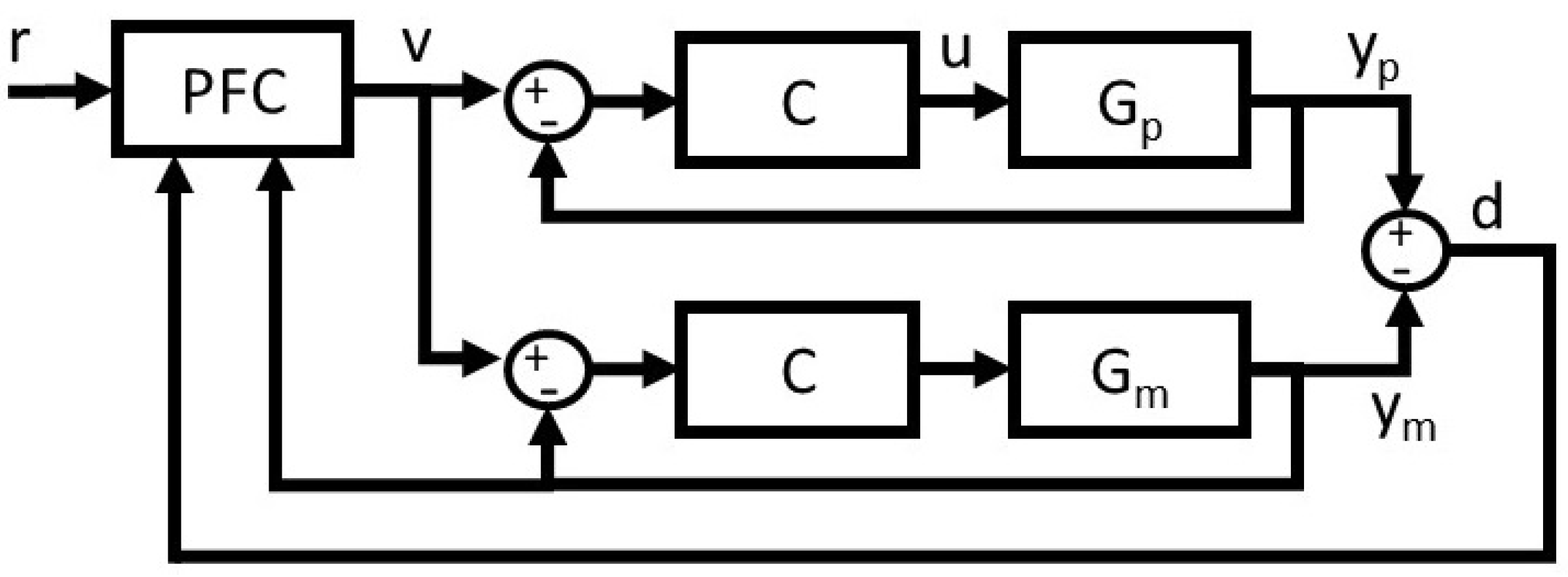
Closed-loop PFC (CLPFC) was proposed to deal with systems which have difficult dynamics and thus are hard or even impossible to tune effectively with more conventional PFC algorithms. The core principle is to modify the original open-loop system by utilising a feedback compensator $C\left(z\right)$ tuned using a suitable method, for instance PID, pole-placement etc, in a cascade configuration as shown in Figure 3. It should be noted, however, Figure 3 is merely a conceptual representation adapted for clarity, and an alternative architecture proposed in [25] is potentially more efficient, especially in the presence of process deadtimes.

In this study, $C\left(z\right)$ is chosen as a standard PID controller, which could be used either to stabilise, damp the oscillations or simply make the system faster to increase the efficacy of the outer PFC tuning parameter $\lambda$. A detailed procedure on how to tune the inner-loop has been discussed in [25,30]. Taking the standard representation, a general discrete PID compensator $C\left(z\right)$ can be represented as:

$$C\left(z\right)=K_p+\frac{K_i{T}_s}{z-1}+K_d\frac{1}{T_f+T_s/(z-1)}$$

(25)

Hence, the inner-loop system is formed as:

$$y_m\left(z\right)=\frac{G\left(z\right)C\left(z\right)}{1+G\left(z\right)C\left(z\right)}v\left(z\right)$$

(26)

A direct relationship between v and the actual system input u can be established as:

$$u_k=C\left(z\right)[v_k-y_{p,k}]$$

(27)

with the new prediction of cascade structure:

$$y_{m,k+n|k}=H_n\underrightarrow{{\displaystyle v_k}}+P_n\underleftarrow{{\displaystyle v_{k-1}}}+Q_n\underleftarrow{{\displaystyle y_{m,k}}}$$

(28)

the new decision variable $v_k$ can be solved using a similar concept as described in the previous section.

The CLPFC law is determined by solving (3) for $v_k$ at every sample by using the modified prediction structure of (28), hence the equality can be formulated as:

$$H_{n}L{v}_k+P_n\underleftarrow{{\displaystyle v_{k-1}}}+Q_n\underleftarrow{{\displaystyle y_{m,k}}}+d_k=(1-{\lambda }^n)r_k+{\lambda }^n{y}_{p,k}$$

(29)

The actual input $u_k$ that will be sent to the plant can be computed by using Equation (27).

Remark 7.

The compensator $C\left(z\right)$ may be implemented based on the nature of a system. If the system is stable without oscillation, then only proportional gain is enough to move the slowest pole near the desired pole. If the system is oscillating or unstable, then the combination between three gains may be used to stabilise or eliminate any oscillation before executing the PFC control law. More details regarding the tuning process and constraint implementation of CLPFC can be found in [25,31].

2.6.4. Closed-Loop Poles with Closed-Loop PFC

Similar to the discussion from Section 2.5, the closed-loop poles of CLPFC can be obtained with suitable modification of parameters $P_{cl}\left(z\right)$,$Q_{cl}\left(z\right)$, and $D_{cl}$, hence:

$$P_{cl}\left(z\right)=b\left(z\right)Q_{cl}\left(z\right)+D_{cl}\left(z\right)a\left(z\right)$$

(30)

3. Proposed PFC Approaches

The previous section has reviewed the recent proposals within the literature to improve the PFC tuning and reliability. It is known that, in general [21,23,25] the tuning parameter $\lambda$ is not as effective as intended (i.e., the closed-loop pole is often not close to $\lambda$) for the core selling point of the algorithm. This lack of efficacy is due to:

• Inappropriate parameterisations of the future input prediction.
• Inappropriate definition of the coincidence point/target trajectory.

Hence, the main proposal of this paper is to draw together the two core insights and hence propose a highly efficient and effective PFC algorithm, whose tuning is both intuitive and effective.

In the simplest terms, the aim is to consider the algorithms of [22,23,25] and replace the control law definition of (3) by (9). The details for how this might be done are presented next and comprise the core contributions of this paper. In both cases the definition of the modified target is the same as given in (8).

3.1. Extending Laguerre PFC to Include a Modified Coincident Point Definition: LFPFC

Predictions with LPFC are given in (21). Combining these with (9) gives the control law as:

$$H_{n}M\theta +H_{n}L{u}_{ss}+P_n\underleftarrow{{\displaystyle u_{k-1}}}+Q_n\underleftarrow{{\displaystyle y_{m,k}}}=T_k$$

(31)

Solving for $u_k$ gives:

$$u_k=u_{ss}-\frac{H_{n}L{u}_{ss}+P_n\underleftarrow{{\displaystyle u_{k-1}}}+Q_n\underleftarrow{{\displaystyle y_{m,k}}}-T_k}{H_{n}M}$$

(32)

Analogously to earlier sections, and again ignoring any $d_k$ terms for the nominal case, this can be represented using z-transforms as:

$$D_{Lf}\left(z\right)u\left(z\right)=N_{Lf}\left(z\right)y\left(z\right)+F_{Lf}r\left(z\right)$$

(33)

Denote this control law as LFPFC.

3.2. Extending Closed-Loop PFC to Included a Modified Coincident Point Definition: CLFPFC

Similar to the previous subsection, the predictions of CLPFC as given in (28) can be combined with (9) to form the new control law of CLFPFC as:

$$H_{n}L{v}_k+P_n\underleftarrow{{\displaystyle v_{k-1}}}+Q_n\underleftarrow{{\displaystyle y_{m,k}}}=T_k$$

(34)

Solving for $v_k$ gives:

$$v_k=\frac{H_{n}L{v}_k+P_n\underleftarrow{{\displaystyle v_{k-1}}}+Q_n\underleftarrow{{\displaystyle y_{m,k}}}-T_k}{H_{n}L}$$

(35)

The manipulated input $u_k$ that will be sent to a plant is then computed as in (27). Analogously to earlier sections, and again ignoring any $d_k$ terms for the nominal case, the z-transforms of control law can be represented as:

$$D_{clf}\left(z\right)u\left(z\right)=N_{clf}\left(z\right)y\left(z\right)+F_{clf}r\left(z\right)$$

(36)

3.3. Discussion of Closed-Loop Stability of the Proposed Algorithms

Several historical papers on PFC, including some of those already cited (e.g., [18]), have analysed the closed-loop stability corresponding to different PFC algorithms. The general consensus is that, with the exception of a few special cases that are often not practically useful, you cannot derive a generic apriori stability guarantee with PFC type approaches and this is a necessary compromise in return for the computational simplicity and ease of implementation. Consequently, one must use a posteriori checks, such as those included in Section 4 of this paper and highlighted in Equations (33) and (36). Having said that, it is also accepted that using sensible coincidence horizons [21] and sensible prediction structures [23], such as those proposed in Section 3, means that closed-loop stability is expected. That is, the best guidance available is to use algorithms such as CLPFC and it would be very surprising if this did not result in closed-loop stability.

This paper focuses mainly on feedforward aspects, e.g., (6), and of course the inclusion of a different feedforward will not impact on the nominal closed-loop stability already discussed in earlier papers. However, it is noted that the change in feedforward also impacts on the use of the disturbance estimate, but again, in the nominal case, $d_k=0$ and thus the nominal behaviour is not affected and one would expect the insights from earlier work to carry across, again emphasising that there is no a priori stability guarantee in general.

4. Numerical Illustrations

This section demonstrates the efficacy of the proposed algorithms given in Section 3 by comparing with existing alternatives. A number of aspects are interesting and will be investigated and for completeness a comparison will cover the following algorithms: (i) Conventional PFC (CPFC); (ii) Laguerre PFC (LPFC); (iii) Closed-loop PFC (CLPFC); (iv) Conventional PFC with feedforward (CFPFC) (v) Laguerre PFC with feed forward (LFPFC); (vi) Closed-loop PFC with feedforward (CLFPFC). Comparisons will be performed for a range of systems with differing dynamics.

The issues of most interest will be those linked to tuning efficacy, that is:

• Proximity to the original target trajectory.
• Disturbance rejection.
• Closed-loop pole positions.

One could argue that proximity to the target trajectory is actually more important than pole position given this matches the concepts assumed by PFC users better.

4.1. Case Studies

Define a 2nd order example (37) with $n=5$ and target pole $\lambda =0.8$,

$$G_1\left(z\right)=\frac{0.1z^{-1}-0.4z^{-2}}{1-1.4z^{-1}+0.45z^{-2}}.$$

(37)

Define a third order example (38) with $n=10$ and target pole $\lambda =0.88$,

$$G_2\left(z\right)=\frac{3.3z^{-1}+0.31z^{-2}-3z^{-3}}{1-2.76z^{-1}+2.54z^{-2}-0.78z^{-3}}.$$

(38)

Define a second order unstable system example (39) with $n=5$ and target pole $\lambda =0.7$,

$$G_3\left(z\right)=\frac{0.2z^{-1}+0.1z^{-2}}{1-1.95z^{-1}+0.9z^{-2}}.$$

(39)

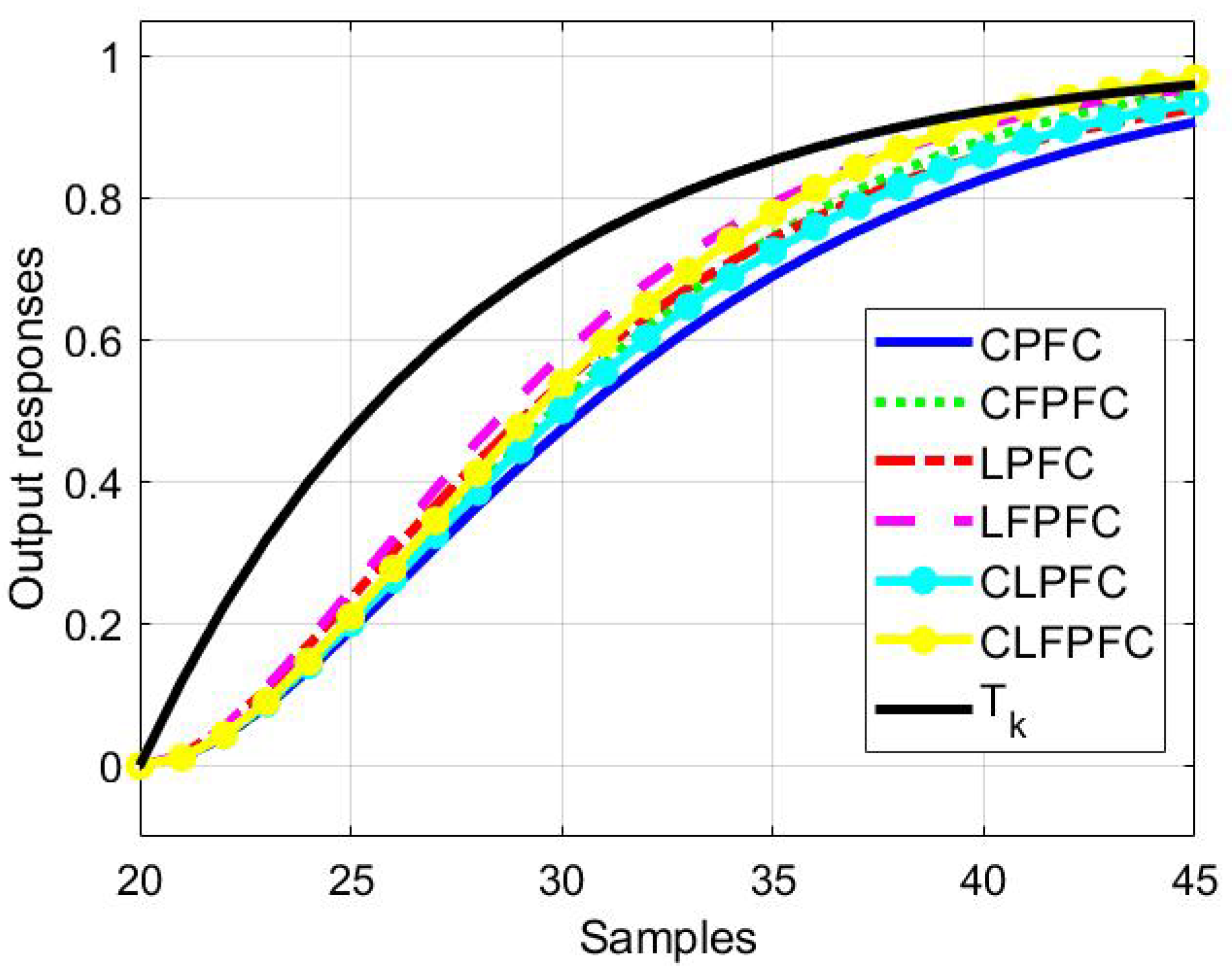
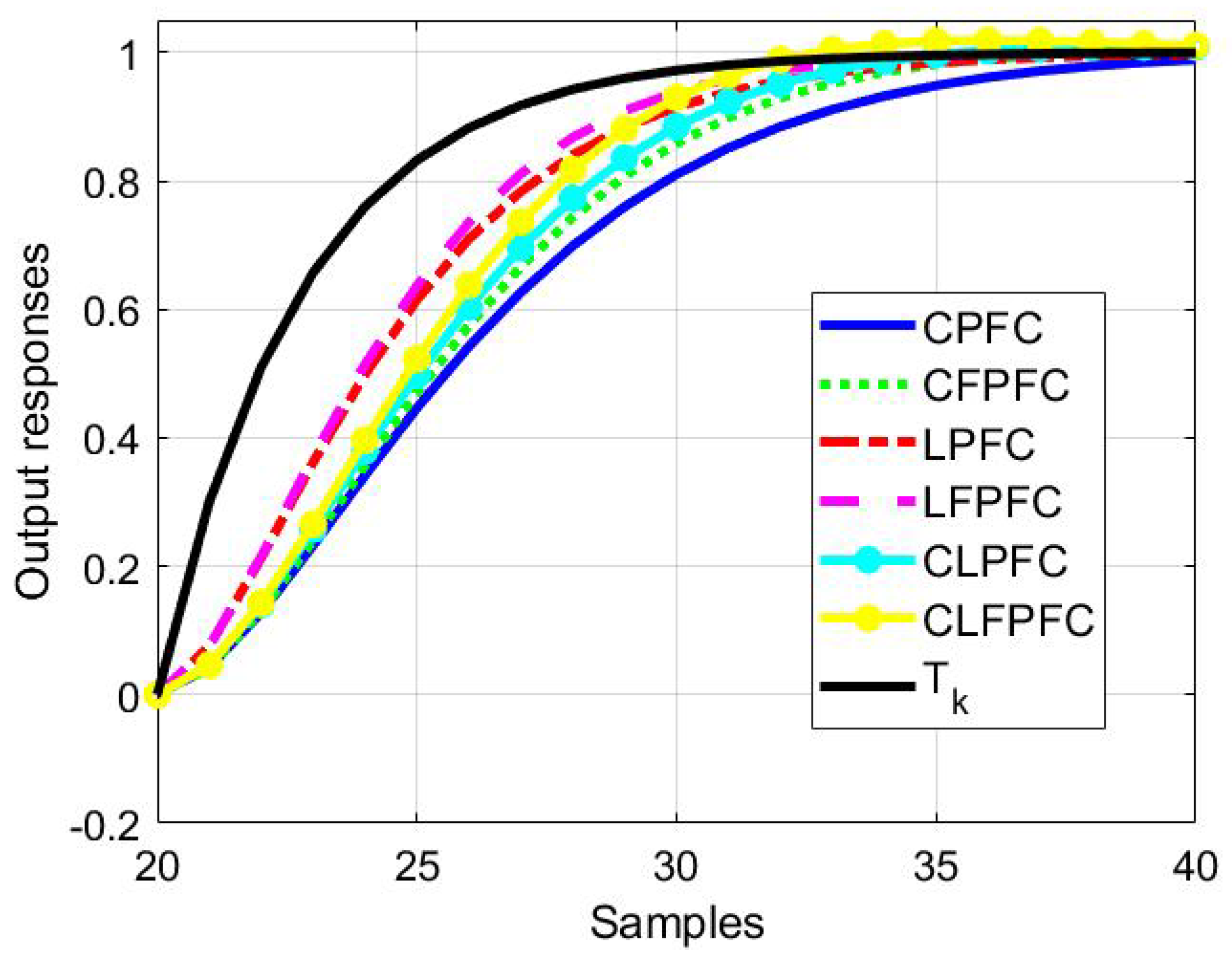
4.2. Comparison of Step Responses with a Target 1st Order Response

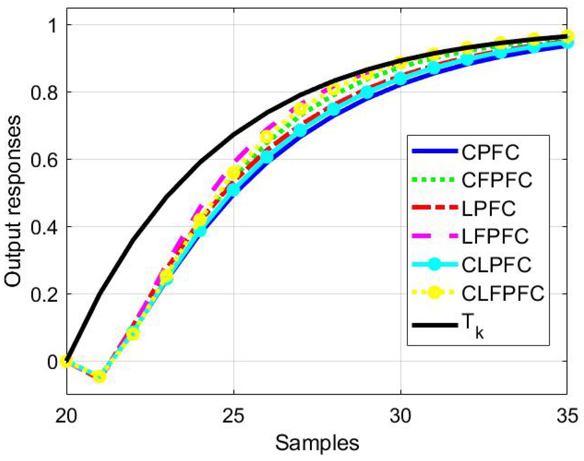
For system $G_1$, the responses to a change in the target are presented in Figure 4. For system $G_2$ (38) the corresponding responses are in Figure 5 and for system $G_3$, the responses are plotted in Figure 6. It should be noted that for CLPFC and CLFPFC, only the proportional gain is used where the values are: $K=-0.1$ for $G_1$, $K=0.001$ for $G_2$ and $K=0.17$ for $G_3$.

For system $G_1$ and $G_2$, the following observations are fairly clear, although more so for the first example; we should also notice at the outset that one will never be able to follow the target closely in immediate transients due to the non-minimum phase attributes of the systems.

• What is most notable is that the approaches deploying the proposed feedforward or change in the coincidence point definition are best at matching the target trajectory.
  • The LFPFC algorithm is the fastest at matching the target $T_k$.
  • The CLFPFC algorithm is the second fastest in matching the target $T_k$ in the initial phase and becomes almost the same with LFPFC in the final stage with a minimum overshot which could be eliminated, if desirable, with more careful tuning of the inner loop.
  • The CFPFC algorithm is the third fastest at matching the target $T_k$.
  • The LPFC algorithm is the fourth fastest at matching the target $T_k$.
  • CLPFC is the fifth fastest at matching the target $T_k$.
  • The conventional PFC algorithm is the worst or slowest at matching the target $T_k$.
• For system $G_3$ as shown in Figure 5, similar observations can be seen except that now the convergence speed of CFPFC becomes the second slowest followed by CPFC.
  • This shows that sometimes improving the matching to the target trajectory alone is not enough to handle the unstable pole in the system. For this case, using the Laguerre algorithm or closed-loop form may improve the response and convergence speed.
  • If this modification is also combined with the new target trajectory, a even better response can be achieved.

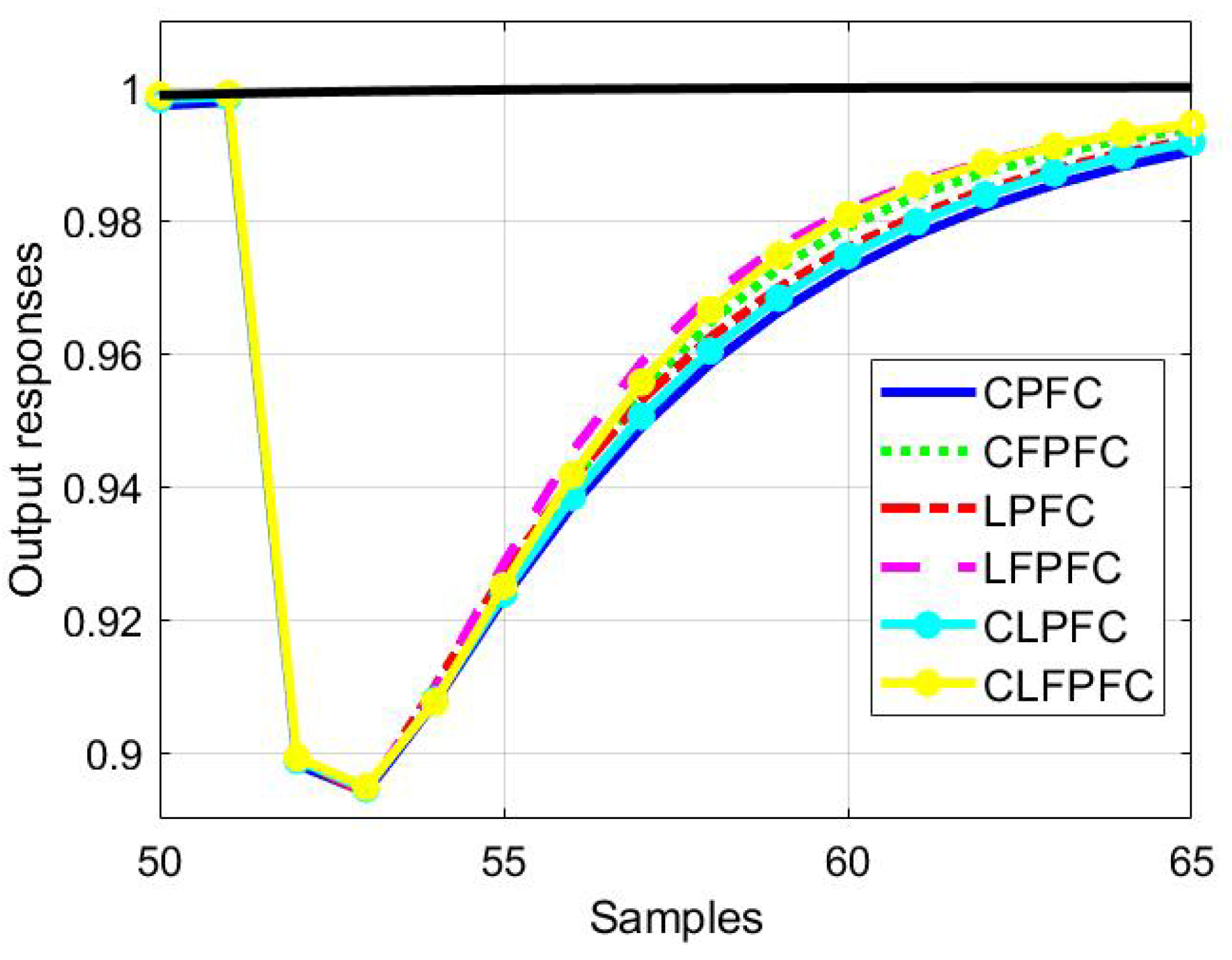
4.3. Disturbance Rejection and Links to $\lambda$

For examples $G_1$, $G_2$ and $G_3$, the responses to an output disturbance are presented in Figure 7, Figure 8 and Figure 9, respectively. For each case, a constant output disturbance with amplitude of −0.1 is inserted at a suitable time. The observations from these results match those in the previous subsection in terms of the ability of the algorithms to reject the disturbance and in particular, how fast they do this compared to the target pole of $\lambda$. This is because the direct link between disturbance and the target trajectory has been established in each control law, particularly in rejecting a constant output disturbance.

4.4. Pole Position Dependence on $\lambda$ and n

One seemingly important observation is to ask how well the system matches the target pole? As hinted at earlier, pole position alone is not the whole picture given the significant role of the feedforward component in the overall behaviour. Before we discuss these further, this section presents the pole positions achieved by each algorithm for each case study, and the given choice of coincidence horizon (we know that changing n can also have an impact, thus there are good and bad choices).

Table 1. Closed-loop poles for system $G_1$ with different PFC algorithms, $n=5$ and $\lambda =0.8$.

Algorithm	CPFC	CFPFC	LPFC	LFPFC	CLPFC	CLFPFC
Poles	$\begin{array}{c}0.812\\ 0.275\end{array}$	$\begin{array}{c}0.55+0.07j\\ 0.55-0.07j\end{array}$	$\begin{array}{c}0.8\\ 0.25\end{array}$	$\begin{array}{c}0.52+0.095j\\ 0.52-0.095j\end{array}$	$\begin{array}{c}0.8\\ 0.32\end{array}$	$\begin{array}{c}0.57+0.14j\\ 0.57-0.14j\end{array}$

,

Table 2. Closed-loop poles for system $G_2$ with different PFC algorithms, $n=10$ and $\lambda =0.88$.

Algorithm	CPFC	CFPFC	LPFC	LFPFC	CLPFC	CLFPFC
Poles	$\begin{array}{c}0.908\\ 0.87\\ 0.832\end{array}$	$\begin{array}{c}0.908\\ 0.85+0.087j\\ 0.85-0.087j\end{array}$	$\begin{array}{c}0.908\\ 0.88\\ 0.753\end{array}$	$\begin{array}{c}0.908\\ 0.813+0.085j\\ 0.813-0.085j\end{array}$	$\begin{array}{c}0.908\\ 0.855+0.043j\\ 0.855-0.043j\end{array}$	$\begin{array}{c}0.908\\ 0.852+0.101j\\ 0.852-0.101j\end{array}$

and

Table 3. Closed-loop poles for system $G_3$ with different PFC algorithms, $n=5$ and $\lambda =0.7$.

Algorithm	CPFC	CFPFC	LPFC	LFPFC	CLPFC	CLFPFC
Poles	$\begin{array}{c}0.76+0.066j\\ 0.76-0.066j\end{array}$	$\begin{array}{c}0.75+0.123j\\ 0.75-0.123j\end{array}$	$\begin{array}{c}0.70\\ 0.62\end{array}$	$\begin{array}{c}0.66+0.113j\\ 0.656-0.113j\end{array}$	$\begin{array}{c}0.77+0.127j\\ 0.77-0.127j\end{array}$	$\begin{array}{c}0.77+0.167j\\ 0.77-0.167j\end{array}$

show the results for system $G_1$, $G_2$ and $G_3$, respectively. Two interesting observations are transparent.

• For examples $G_1$ and $G_2$, despite not tracking the target as well, the algorithms using the control law definition of (3) such as CPFC, LPFC and CLPFC achieve poles close to the target pole. Although the algorithms with the new control law definition of (9) such as CFPFC, LFPFC and CLFPFC seem to be far from the desired pole, yet these algorithms have relatively very fast remaining poles which give convergence within a few samples.
• As for example $G_3$ with unstable dynamics, the algorithms without pre-stabilisation such as CPFC and CFPFC have slower real poles compared to the desired pole with small imaginary poles. As for LPFC and LFPFC, both have a faster poles than the desired pole. For CLPFC and CLFPFC, although the real poles are slower, these provide a suitable convergence speed to match the target pole as shown in Figure 6. This scenario in return will give a minimum overshoot on the response.

One might assume from the observation of example $G_1$ and $G_2$ that the orginal PFC law is doing a better job, although of course Figure 4, Figure 5, Figure 6, Figure 7 and Figure 8 contradict this. What is actually happening is that the dynamics for control law (9) are essentially being enforced through the feedforward component, and the remainder of the control or feedback part then has relatively fast poles.

In summary, given the closed-loop behaviour arises from a combination of feedforward and feedback, it seems that the actual position of the closed-loop poles is not as critical as one might have expected. More work is needed here to understand the consequences, if any, of the widely varying poles seen in Table 1, Table 2 and Table 3.

5. Conclusions

This paper makes an important contribution to the family of efficient MPC laws and in particular to predictive functional control algorithms. It has been shown how an earlier work on improving the definition of the coincident point used in a PFC control law can be applied to more recent variants such as Laguerre PFC and closed-loop PFC. Further benefits accrue, although these are less significant than those with the conventional PFC. Hence, a combination of re-parameterising the degrees of freedom alongside a more consistent definition of the coincidence point produces a PFC algorithm which gives much more consistent behaviour and thus delivers what the original proposers of PFC most wanted, that is, a closer and simpler link between a user specified behaviour and the one actually achieved. However, one interesting observation is that the resulting closed-loop poles appear much faster than the target behaviour, apparently because of the further influence of the proposed feedforward component on the improved Laguerre and closed-loop PFC variants.

In terms of future work the most obvious issue that needs investigation is sensitivity. The approach proposed in this paper provides simple and intuitive tuning for non-expert users, but this could potentially be at the cost of worse sensitivity to uncertainty. Certainly, the appearance of faster poles may indicate worse sensitivity, but the various interactions within the control law using independent models imply part of the feedforward component is, in effect, also acting within the feedback loop, which is indeed not clear cut.

References

- Qin, S.; Badgwell, T.A. A survey of industrial model predictive control technology. Control Eng. Pract. 2003, 11, 733–764. [Google Scholar] [CrossRef]
- Mayne, D.Q. Model predictive control: Recent developments and future promise. Automatica 2014, 50, 2967–2986. [Google Scholar] [CrossRef]
- Eduardo, F.; Camacho, C.B.A. Model Predictive Control; Springer: London, UK, 2007. [Google Scholar]
- Clarke, D.W.; Mohtadi, C.; Tuffs, P.S. Generalized predictive control—Part I. The basic algorithm. Automatica 1987, 23, 137–148. [Google Scholar] [CrossRef]
- Rawlings, J.B.; Mayne, D.Q. Model Predictive Control: Theory and Design; Nob Hill Publishing: Madison, WI, USA, 2009. [Google Scholar]
- Rossiter, J.A. A First Course in Predictive Control; CRC Press: Boca Raton, FL, USA, 2018. [Google Scholar]
- Schwenzer, M.; Ay, M.; Bergs, T.; Abel, D. Review on model predictive control: An engineering perspective. Int. J. Adv. Manuf. Technol. 2021, 117, 1327–1349. [Google Scholar] [CrossRef]
- Köhler, J.; Müller, M.A.; Allgöwer, F. Analysis and design of model predictive control frameworks for dynamic operation—An overview. Annu. Rev. Control 2024, 57, 100929. [Google Scholar] [CrossRef]
- Kouramas, K.; Faísca, N.; Panos, C.; Pistikopoulos, E. Explicit/multi-parametric model predictive control (MPC) of linear discrete-time systems by dynamic and multi-parametric programming. Automatica 2011, 47, 1638–1645. [Google Scholar] [CrossRef]
- Algower, F.; Zheng, A. Nonlinear Predictive Control; Birkhauseer: Basel, Switzerland, 2010. [Google Scholar]
- Kolmanovsky, I.; Garone, E.; Di Cairano, S. Reference and command governors: A tutorial on their theory and automotive applications. In Proceedings of the American Control Conference, Portland, OR, USA, 4–6 June 2014. [Google Scholar]
- Bemporad, A.; Morari, M.; Dua, V.; Pistikopoulos, E.N. The explicit linear quadratic regulator for constrained systems. Automatica 2002, 38, 3–20. [Google Scholar] [CrossRef]
- Richalet, J.; O’Donovan, D. Predictive Functional Control: Principles and Industrial Applications; Springer: Berlin/Heidelberg, Germany, 2009. [Google Scholar]
- Richalet, J.; Rault, A.; Testud, J.L.; Papon, J. Model predictive heuristic control: Applications to industrial processes. Automatica 1978, 5, 413–428. [Google Scholar] [CrossRef]
- Richalet, J.; Donovan, D.O. Elementary Predictive Functional Control: A tutorial. In Proceedings of the International Symposium on Advanced Control of Industrial Processes, Hangzhou, China, 23–26 May 2011; pp. 306–313. [Google Scholar]
- Khadir, M.; Ringwood, J. Extension of first order predictive functional controllers to handle higher order internal models. Int. J. Appl. Math. Comp. Sci. 2008, 18, 229–339. [Google Scholar] [CrossRef]
- Khadir, M.T. Enthalpy predictive functional control of a pasteurisation plant based on a plate heat exchanger. In Proceedings of the 2007 European Control Conference (ECC), Kos, Greece, 2–5 July 2007; IEEE: Piscataway, NJ, USA, 2007. [Google Scholar] [CrossRef]
- Richalet, J. Industrial applications of model based predictive control. Automatica 1993, 29, 1251–1274. [Google Scholar] [CrossRef]
- Jing, W.X.; Zhen, L.M.; Shuai, C.; Hao, L.; Wang, X. PID–PFC control of continuous rotary electro-hydraulic servo motor applied to flight simulator. J. Eng. 2019, 2019, 138–143. [Google Scholar] [CrossRef]
- Rossiter, J.A. A priori stability results for PFC. Int. J. Control 2016, 90, 305–313. [Google Scholar] [CrossRef]
- Rossiter, J.A.; Haber, R. The effect of coincidence horizon on predictive functional control. Processes 2015, 3, 25–45. [Google Scholar] [CrossRef]
- Rossiter, J.A.; Abdullah, M. Improving the use of feedforward in Predictive Functional Control to improve the impact of tuning. Int. J. Control. 2022, 95, 1206–1217. [Google Scholar] [CrossRef]
- Abdullah, M.; Rossiter, J.A.; Haber, R. Development of constrained predictive functional control using Laguerre function based prediction. IFAC-PapersOnLine 2017, 50, 10705–10710. [Google Scholar] [CrossRef]
- Rossiter, J.A. Input shaping for PFC: How and why? J. Control Decis. 2015, 3, 1–14. [Google Scholar] [CrossRef]
- Aftab, M.S.; Rossiter, J.A. Predictive functional control for challenging dynamic processes using a simple prestabilization strategy. Adv. Control Appl. 2022, 4, e102. [Google Scholar] [CrossRef]
- Zhang, Z.; Rossiter, J.A.; Xie, L.; Su, H. Predictive functional control for integral systems. In Proceedings of the International Symposium on Process System Engineering, San Diego, CA, USA, 1–5 July 2018. [Google Scholar]
- Rossiter, J.A.; Aftab, M.S. Recent Developments in Tuning Methods for Predictive Functional Control. Processes 2022, 10, 1398. [Google Scholar] [CrossRef]
- Maciejowski, J.M. Predictive Control with Constraints; Pearson Education: London, UK, 2002. [Google Scholar]
- Wang, L. Model Predictive Control System Design and Implementation Using MATLAB®; Springer: London, UK, 2009. [Google Scholar]
- Aftab, M.S.; Rossiter, J.A. Predictive Functional Control with Explicit Pre-conditioning for Oscillatory Dynamic Systems. In Proceedings of the 2021 European Control Conference, Virtual, 29 June–2 July 2021. [Google Scholar]
- Abdullah, M.; Rossiter, J.A. Alternative method for Predictive Functional Control to handle an integrating process. In Proceedings of the 2018 UKACC 12th International Conference on Control (CONTROL), Sheffield, UK, 5–7 September 2018; IEEE: Piscataway, NJ, USA, 2018; pp. 26–31. [Google Scholar]