Abstract
This study presents an aerostructural optimization process for wind turbine blades aimed at enhancing the turbine’s performance. The optimization framework integrates DAFoam as the computational fluid dynamics (CFD) solver, TACS as the finite element method (FEM) solver, Mphys for fluid–structure coupling, and SNOPT as the optimizer within the OpenMDAO framework. The objective is to simultaneously increase the torque generated by the wind turbine while decreasing the mass of the blade, thereby improving its efficiency. The design variables in this optimization process are the blade shape and panel thickness. The aerodynamic objective function is torque, a key performance indicator for wind turbine efficiency. The structural objective function is the blade mass, as reducing mass is essential to minimize material and manufacturing costs. The optimization process utilizes the integrated capabilities of DAFoam, TACS, Mphys, and SNOPT to iteratively evaluate and modify the blade shape and panel thickness. The OpenMDAO framework facilitates seamless communication between the solvers and the optimizer, ensuring a well-coordinated, efficient optimization process. The results of the optimization show a 6.78% increase in torque, which indicates a significant improvement in the wind turbine’s energy production capacity. Additionally, a 4.22% decrease in blade mass demonstrates a successful reduction in material usage without compromising structural integrity. These findings highlight the potential of the proposed aerostructural optimization process to enhance the performance and cost-effectiveness of wind turbine blades, contributing to the advancement of sustainable energy solutions. This work represents the first attempt to implement DAFoam for wind turbine aerostructural design optimization.
1. Introduction
The development of renewable energy sources has become a priority for emerging nations because of the volatile energy market, the depletion of fossil fuels, and deteriorating environmental conditions. The fundamental idea behind using renewable energy is that it comes from ongoing natural processes. As a result, emerging nations reject the use of fossil fuels and migrate to other sources of energy like wind and solar. The majority of these renewable energy sources significantly reduce CO2 emissions, as suggested by the Intergovernmental Panel on Climate Change (IPCC) [1].
Renewable energy is produced from natural resources that replenish themselves naturally and without human intervention. Wind energy is one of the renewable energy sources that is growing the quickest. As a result, harnessing wind energy to generate electricity is more economical than using coal or gas-fired power plants. Despite all of its advantages, wind energy’s main disadvantage is that power is intermittent. Consequently, another energy source that can be produced on demand must be combined with wind energy. Wind power should be considered an additional energy source rather than the main one.
Only land-based wind power can economically meet humanity’s energy demands, claim Zhou et al. [2]. However, only a tiny fraction of this enormous potential for wind energy is now being used [3]. Three thousand years of human history have seen the utilization of wind energy [4]. The use of wind energy peaked during both World Wars, then decreased afterward and again rose as a result of the demise of the petroleum sector in the 1970s [5]. Moreover, modern wind turbines had been built in Denmark by the end of the seventeenth century [6]. The technological complexity of wind turbines makes them difficult to run with a variety of workloads [7].
Expanding the usage of carbon-free technologies that rely on high-potential, renewable energy sources like wind power would require lowering the levelized cost of energy. Modern, highly flexible wind turbine rotors are defined by strongly coupled, multi-physics interactions, which must be captured using advanced computational approaches. As a consequence, computing methods may greatly improve the time-consuming process that occurs in wind turbine blades.
The remainder of this paper starts with a literature review on the aerostructural optimization of wind turbine blades in Section 2, followed by the methodology on the aerodynamic optimization, structural optimization, and fluid–structural coupling processes of the aerostructural optimization in Section 3, and the main findings are presented and discussed in Section 4. Finally in Section 5, the conclusion is made.
2. Literature Review
Energy is crucial for social and economic progress, and because of rising greenhouse gas emissions and fuel costs, renewable energy sources are gaining popularity. Renewable energy does have certain limitations, too, such intermittent generation and the need for sophisticated design, planning, and control optimization techniques.
Computational optimization techniques for renewable energy design, planning, and control difficulties were demonstrated by Baos et al. in 2011 [8]. The use of heuristic approaches, Pareto-based multi-objective optimization, and parallel processing are intriguing study areas in renewable and sustainable energy, according to one of the review’s fascinating results.
A bibliography on wind speed and wind power projections was eventually provided by Lei et al. [9]. The incorporation and application of artificial intelligence techniques as well as the blending of diverse statistical models for both long- and short-term forecasts were seen as possible prospects. The papers listed below [10,11,12,13] discuss forecasting techniques for wind energy.
Miller et al. [14] reviewed recent developments in numerical simulation techniques, technology, and applications to wind energy. They also looked at past numerical simulations.
The wind energy business heavily relies on computational fluid dynamics to research innovative turbine designs (CFD). New tools must be created in order to apply CFD early in the design phase, where lower-fidelity methods like blade element momentum (BEM) are more common. Algorithmic optimization tools are extremely helpful since they reduce the dependency on trial-and-error design.
Over the past ten years, a number of tools for designing wind turbines have been created. The entire turbine system, including aerostructural rotor and tower models, the power generator, and fixed-bottom foundations or floating platforms, is simulated using state-of-the-art software, such as Open-FAST [15], Cp-Max [16], HAWTopt2 [17], ATOM [18], SHARPy [19], Qblade [20], and MoWit [21].
Various traditional tools employ a mix of models of different accuracy levels to analyze different parts of a system. OpenFAST, a turbine analysis standard [15], integrates a modal and multibody dynamics framework that encompasses all major components. This system, utilizing BeamDyn and ElastoDyn modules, employs beam models to capture the turbine’s dynamic response. However, these modules have limitations in terms of degrees of freedom (ElastoDyn) and accuracy of local stress values (ElastoDyn and BeamDyn). OpenFAST’s aerodynamic forecasts through BEMT-based AeroDyn align well with traditional designs but face challenges with larger blades showing significant deflections and 3D effects.
Madsen et al. [22] and concurrent research employing a blade-resolved rotor model also overlooked the hub geometry. However, computational fluid dynamics (CFD) analyses effectively capture spanwise and tip flow phenomena, significantly impacting in-plane and off-plane loads. Horcas et al. [23] demonstrated that a tool based on OpenFAST’s physical models, HAWC2, tends to overpredict loads on a 10 MW turbine at wind speeds below the rated threshold and underestimates the advantages of curved wing tips, even with a steady power curve. Additionally, tools like OpenFAST lack accuracy in computing gradients, hindering their use in numerical optimization. They also rely on precomputed wing section drag polars, limiting the optimization of airfoil shapes.
Efforts have been made to combine high- and low-fidelity tools to strike a balance between accuracy and computational expense. Ramos-García et al. [24] coupled finite-element structural models with a hybrid lifting-line–vortex method, showing agreement with Heinz et al. [17]. While this approach overcomes some limitations of BEMT at a lower cost than blade-resolved solvers, its application remains primarily limited to analyses due to challenges in computing derivatives.
Other recent endeavors focused on a narrower but higher-fidelity approach to capture the intricate fluid–structure interaction of turbine blades [25]. Wainwright et al. [26] merged a commercial CFD software package and a finite element modal solver using GPU acceleration to study a rotor’s aerostructural behavior in the wake of an upstream turbine. Cheng et al. [27] validated a model coupling different solvers in OpenFOAM to study a floating wind turbine’s behavior. However, while high-fidelity codes offer accuracy, they suffer from computational cost and implementation complexity, restricting their use for optimization.
Research on applying numerical analysis tools to wind turbine optimization problems has been undertaken by Gray et al. [28], Ning and Petch [29], and Ingersoll and Ning [30]. Bortolotti et al. [31] developed a design space exploration strategy efficiently sizing the rotor at a conceptual design stage, though it could not exploit tradeoffs between aerodynamic and structural design. Bottasso et al. [32] proposed a bilevel design approach using a comprehensive turbine model, maximizing annual energy production over mass, but with limitations in accuracy and robustness.
Low-fidelity aerostructural optimization for wind turbine blades generally involves simplifications and approximations in representing the complexities of fluid–structure interactions and the aerodynamics of the blades. These limitations impact the accuracy and robustness of the optimization process compared to high-fidelity approaches.
For high-fidelity aerodynamic shape optimization, the adjoint technique is an effective method for calculating the derivatives of an interest function with respect to a large number of design factors.
In addition, proposed the theory and architecture of OpenMDAO in 2019 [16]. This open-source multidisciplinary design optimization (MDO) framework solves coupled systems utilizing Newton-type algorithms and takes use of problem structure via novel hierarchical methodologies. The main goal of MDO is to build interconnected numerical models of challenging engineering systems. There are a number of MDO software frameworks; however, none of them completely makes use of cutting-edge methods to solve connected models efficiently.
This study’s goal is to present an aerostructural optimization method for wind turbine blade design that aims to maximize torque while lowering mass because none of the earlier literature studies have attempted to incorporate the associated performance optimization of wind turbines. While structural optimization aims to minimize bulk while maintaining structural integrity, aerodynamic optimization concentrates on altering the shape of the blade. This approach is crucial for the widespread adoption of wind energy systems since it is both effective and affordable.
3. Materials and Methods
3.1. Baseline Wind Turbine Blades
The optimization is based on the NREL Phase VI geometry, which was created for applied CFD validation tests, with the two-bladed 10.058 m diameter NREL Phase VI Rotor based on the S809 airfoil [33]. Figure 1 illustrates the baseline geometry of the airfoil, which is replotted based on Hand et al. [33].
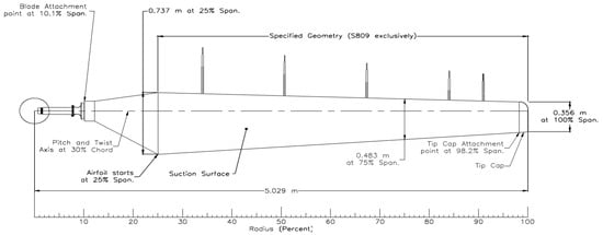
Figure 1.
Blade geometry [33].
The design process involved thorough evaluations of tradeoffs, considering nonlinear changes in taper and twist patterns, as well as the integration of extra airfoils. The result is a blade featuring a consistent taper and a twist distribution that varies in a nonlinear manner, using the S809 airfoil from the base to the tip. This initial design provides a good foundation for optimization and offers the possibility of achieving even better performance.
3.2. Aerostructural Optimization Framework
In spite of having a higher computational cost and implementation effort when compared to low-fidelity solvers, the use of high-fidelity solvers in aerostructural design optimization of wind turbine blades can provide improved accuracy and more complete model specification. To manage the high-dimensional and high-fidelity optimization formulations in a tractable numerical problem, gradient-based optimization techniques are required, such as the use of adjoint-based derivative computations. Multiple aerostructural, hydrostructural, aerothermal, aeropropulsive, and aeroelastic MDO issues have been incorporated in the OpenMDAO framework to handle interdisciplinary design optimization challenges in engineering systems [34]. The main functionality of the Python-based, open-source, high-performance computing platform known as OpenMDAO is gradient-based optimization using analytic derivatives. The implementation presented in this paper is based on a two-way fluid–structure interaction (FSI) in the OpenMDAO framework that couples the discrete adjoint with OpenFOAM for high-fidelity multidisciplinary design optimization (DAFoam) [35] and the Toolkit for the analysis of composite structures (TACS) [36] with Mphysics [37]. With competitive speed, scalability, and accuracy, DAFoam employs a discrete adjoint technique without Jacobians. It also offers a Python interface for linking interdisciplinary design optimization.
In this study, we optimize the aerostructural design of wind turbine blades to improve their aerodynamic performance and decrease their mass using the discrete CFD solver DAFoam in combination with the OpenMDO framework. The aerodynamic and structural systems work together; the aerodynamics group receives a mesh as input and creates aerodynamic loads as an output, while the structural group receives these loads as input and generates structural displacements as a result. This method has received a lot of previous research attention, with several studies examining its potential applications in the optimization of aircraft aerodynamics and aerostructural design [34,38,39].
According to the extended design structure matrix (XDSM) schematic [40] in Figure 2, the MACH [34] is a group of closely connected submodules that enable geometry parametrization and deformation, coupled aerostructural analysis, and effective derivatives assessment in an optimization context.
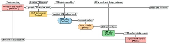
Figure 2.
MACH optimization framework’s XDSM diagram.
The OpenMDAO framework, which is based on Mach-aero, is used to carry out the optimization procedure [41]. The creation of the structural mesh in MSC Patran and the aerodynamic mesh in pyHyp are both part of the preprocessing stage. In terms of aerodynamic optimization, during the preprocessing stage, we create the CFD mesh for the baseline design surface geometry. To do this, we first create the surface mesh using ICEM CFD and then extrude it to create the volume mesh using pyHyp. Additionally, we use the ICEM CFD to create the freeform deformation (FFD) control points for geometry parameterization. The first geometric design variables (FFD points displacement) will then be passed to the geometry parameterization module pyGeo by the optimizer (SNOPT). An open-source FFD tool for parameterizing the geometry of the design surface is called PyGeo. A series of point clouds may be embedded using pyGeo into the designated FFD box, and the point cloud can then be deformed by rearranging the FFD coordinates. Both organized and unstructured meshes may be used with pyGeo. The CFD design surface and surface mesh will be entirely contained in the FFD box that is produced during the preprocessing stage. The updated design surface is subsequently sent to the IDWarp mesh deformation module. Using an inverse-distance weighting method, IDWarp is an open-source mesh deformation tool that may be used to reshape high-quality volume mesh according to the new design surface. As opposed to regenerating the volume mesh, we can eliminate numerical noise by using IDWarp, which is smooth while deforming the volume mesh. Updated volume mesh is passed to the CFD solver via IDWarp (OpenFOAM). After solving the flow, OpenFOAM provides the adjoint solver component with the converged CFD state variables. The aerodynamic objective and constraint functions are likewise computed using OpenFOAM (e.g., power, thrust). Ultimately, the adjoint solver returns the total derivatives of the constraint and goal functions to the optimizer after computing them. The function values and derivatives are used by the optimizer to update the design variables for the subsequent optimization iteration. The optimization process keeps going until it converges.
OpenMDAO/MPhys is used in the aerostructural optimization framework. The aerodynamic-only and aerostructural optimization frameworks are comparable, with the following exceptions: The whole FEM mesh and the CFD design surface are included in the FFD box. Therefore, in order to guarantee a constant fluid–structure interface, pyGeo deforms both the FEM mesh and the CFD surface mesh; the aerostructural analysis module includes an integrated mesh deformation module; the aerostructural optimization conducts coupled aerostructural analysis and adjoint, which is needed to solve the CFD and FEM systems utilizing block Gauss–Seidel techniques, as opposed to single-discipline analysis; aerodynamic and structural variables, such as power, thrust, aggregated von Mises stress, and structural mass, are included in the objective and constraint functions that are returned to the optimizer.
TACS and OpenFOAM solvers are used in the aerostructural study. The baseline CFD and FEM meshes, CFD and FEM design variables, and the most recent design surface geometry (blade geometry) in the optimization loop are the inputs (e.g., blade rotation speed). The converged aerostructural state variables, such as pressure, velocity, and structural displacement, as well as the objective and constraint functions, are the outputs (e.g., power and thrust). The primary driving force behind the aerostructural analysis process is the computation of the updated CFD surface mesh using the geometry of the design surface and the CFD surface mesh displacement derived from the displacement transfer component (in the first iteration, the displacement is zero). The updated CFD volume mesh is then computed by the mesh deformation component using the updated CFD surface mesh. The updated CFD volume mesh is then sent to the CFD solver component, which runs flow field simulations, extracts the CFD surface force, and sends it to the load transfer component. The FEM solver receives the force from the load transfer component, which interpolates the CFD surface force to the FEM surface force. The structural displacement is then calculated by the FEM solver component, which also extracts the FEM surface displacement and feeds it to the displacement transfer component. After interpolating the FEM surface displacement to the CFD surface displacement, the displacement transfer component delivers the data to the aerostructural analysis primary driver to initiate the subsequent iteration. Until the residuals for the FEM and CFD solvers are smaller than the recommended tolerances, the aforementioned procedure is repeated.
The “Scenario” generic aerostructural template from MPhys makes the aforementioned interaction between CFD and FEM solvers easier. To expand the aerostructural situation, a Python interface known as mphys dafoam is available that utilizes OpenFOAM and DAFoam as the CFD and adjoint solvers (the adjoint is elaborated on in the next section). An opensource inverse distance weighted mesh deformation algorithm called IDWarp is used by the mesh deformation component. The adjoint-based gradient evaluation tool FUNtoFEM and a general aeroelastic analysis tool named Meld are the sources of the load and displacement transfer components. As the FEM solver, TACS is employed. Using an Aitken relaxation technique, the nonlinear block Gauss–Seidel solver in OpenMDAO is used to do the CFD and FEM iteration. Figure 3 depicts the entire aerostructural optimization profile.
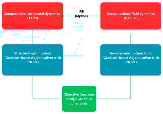
Figure 3.
Profile for multidisciplinary design optimization.
3.3. RANS-Based Turbulent Simulation
For the conservation of mass and momentum, the Navier–Stokes equations are used to describe a three-dimensional steady incompressible flow.
These equations are given as Equations (1) and (2), where denotes the fluid’s velocity, denotes its pressure, denotes its density, denotes its dynamic viscosity. The Spalart–Allmaras model [42] is employed as the turbulence model because it is reliable, effective, converges well, and is simple to use. In Table 1, the boundary conditions are displayed. The initial values for k, ε, νt, ω, ṽ are 0.8375 m2/s2, 0.2 m2/s3, 5 × 10⁻⁵ m2/s, 12.24 s−1, and 5 × 10⁻⁵ m2/s, respectively. The inlet velocity of the fluid is 7 m/s, and the blade has a rotational velocity of 72 rpm. The initial values for the boundary conditions are calculated based on the turbulence free-stream boundary conditions.

Table 1.
Boundary conditions.
In our study, the computational domain is a spherical shape with the blade located at the center of the spherical far-field domain, as shown in Figure 4, where the radius of the blade is 5.029 m while the radius of the spherical domain is 20 times the blade’s radius, and the entire spherical domain is defined as inlet–outlet.
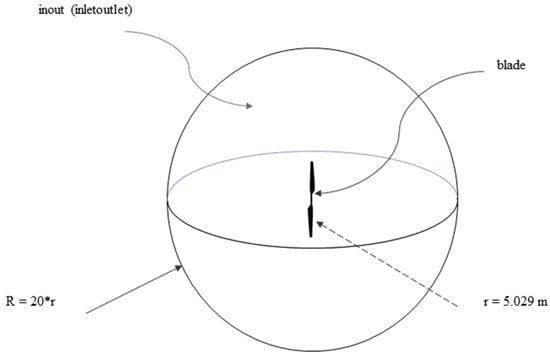
Figure 4.
Computational domain and boundary conditions.
As for the turbulence model, as mentioned above, a one-equation Spalart–Allmaras model is used because we have limited computational power. It encompasses the resolution of just a single transport equation, specifically the one for kinematic turbulent viscosity. As a result, the computational workload is reduced when compared to popular two-equation models such as k-epsilon. The S-A model has undergone thorough validation for external flows and demonstrates strong alignment with experimental findings in aerospace applications.
3.4. Structural Model
The influence of temperature is not included in the structural simulation employed in this model. As a result, the simulation is be set to isothermal for this chapter. The state equation for the momentum balance has the following structure:
where and are displacement vector and stress tensor, respectively, while and are the material properties. The stress tensor is specified using strain tensor and there is transpose operation:
Equations (4) and (5) when combined provide the following results:
The tweak to the solution technique improves the convergence of a simulation by rearranging terms in Equation (6). The first component of Equation (3) is implicitly solved using OpenFoam, whereas the second term is explicitly solved.
Therefore, by changing the order of phrases, the explicit and implicit components are more evenly distributed. Equation (3) in its modified form has the following form:
The traction force boundary condition has the following expression (where is a surface normal to the boundary):
Only elastic deformation is described by Equations (3)–(8). Every substance in nature experiences plastic deformation after it has been subjected to a certain amount of stress. The following is the format of the modified governing equation with plastic term:
where and are incremental displacement vector and incremental plastic strain tensor, respectively. Equation (10) undergoes similar modification:
3.5. Discrete Adjoint Derivative Computation
The torque in our example serves as the objective function , and is the vector of design variables. The adjoint method is utilized to quickly determine the total derivatives . In the discrete technique, it is expected that the primary solver can provide a discretized form of the governing equations and that the design variable vectors and satisfy the discrete residual equations = 0, where R is the residual vector.
Therefore, the relevant functions are functions of the state variable as well as the design variable: . Although there are several functions of relevance, is regarded as a scalar in the following derivations to retain generality. Each new function demands the solution of an additional adjoint system, as becomes evident later. The total derivative is derived using the chain rule:
when there are no implicit computations, making the estimation of the partial derivatives and very simple. On the other hand, because it is implicitly specified by the residual equations , the total derivative matrix is expensive.
We may obtain using the chain rule for R. We may then exploit this information to our advantage because the governing equations should always hold. Therefore, the derivatives must amount to zero:
In Equation (12), substituting from Equation (11) yields:
We may solve the adjoint equation by transposing the state Jacobian matrix and using, as the right-hand side.
The adjoint vector is the . When we enter the adjoint vector into Equation (13) after solving this equation, we obtain the total derivative, which is expressed as:
Since the design variable is not explicitly stated in Equation (14), we only need to solve the adjoint equations once for each function of interest. As a result, its computing cost is related to the number of interesting functions rather than being independent of the number of design variables. This strategy, known as the adjoint technique, provides benefits for many design issues in aeronautical engineering when just a small number of functions are of relevance but where several hundred design variables may be used.
The following four essential steps make up a discrete adjoint implementation, which involves computing the partial derivatives and resolving the adjoint equations:
- (1)
- Figuring out the partial derivatives and
- (2)
- The adjoint vector in the linear Equation (13) solution.
- (3)
- The method of computing the partial derivatives and .
- (4)
- Calculate the total derivative using Equation (15).
The four approaches outlined above do not need a specific residual function ; therefore, they may be used with any collection of discrete PDEs.
3.6. Aerostructural Coupling
The adjoint formulation indicated above assumes that the state variables of the finite element method (FEM) and computational fluid dynamics (CFD) are combined and solved concurrently, which results in a bigger Jacobian matrix and increased memory use. To get around this, we solve the aerostructural adjoint in a linked way using a different technique called block Gauss–Seidel, as shown below.
The abbreviations CFD and FEM, which stand for computational fluid dynamics and finite element method, respectively, refer to the residual and state variables for the solvers. We use DAFoam to solve the CFD adjoint equation:
According to Kenway et al.’s study [43], DAFoam uses a technique known as Jacobian-free adjoint, where automated differentiation is employed to compute partial derivatives and matrix–vector products. DAFoam employs the generalized minimum residual (GMRES) iterative linear equation solver from the PETSc package to solve the adjoint equation [44]. DAFoam employs a layered technique using the additive Schwartz method for global preconditioning, and an incomplete lower and upper (ILU) factorization method with one level of fill-in is utilized for local preconditioning.
The preconditioner matrix is produced to improve convergence by estimating the residuals and linearizing them [45]. Since constructing takes up around 30% of the adjoint runtime, this matrix is only created once and then utilized for the adjoint equation. This results in a considerable decrease in adjoint runtime. The adjoint equation for the FEM component is solved using TACS:
Without explicitly creating the matrix, automated differentiation is used to determine the nondiagonal portions of the matrix multiplied by a vector.
Using OpenMDAO and MPhys, the aerostructural system was created in a modular manner for adaptability. The components in Figure 1 needed to multiply the state Jacobian matrix by a particular vector and implement ways to compute output based on input. The adjoint total derivative computation was unified with OpenMADO using the MAUD algorithm [46]. In OpenMDAO, a linear block Gauss–Seidel solver with Aitken relaxation was employed to solve the coupled adjoint of CFD and FEM.
3.7. Baseline Geometry Configuration for Aerostructural Optimization
As in our earlier research [47], we used the NREL Phase VI, which has just two blades, as the baseline geometry in this investigation. Regarding the aerodynamic component, the surface mesh as shown in Figure 5c is constructed in ICEM CFD, and the spherical volume mesh as shown in Figure 5a is created by extruding the structured surface mesh using the opensource mesh generator pyHyp [48]. Figure 5b depicts the hyperbolic expansion layer that surrounds the wind turbine blade. Additionally, MSC Patran generates a structural finite element mesh that matches the shape of the outer mold line and incorporates an interior main shear web as seen in Figure 5d. The whole collection of structural elements is made up of thin CQUAD hexahedral shell elements. At the root, which is situated at a distance of about 0.66 from the rotating axis, two identical blades are fastened. In Figure 5e, the FFD points for the aerodynamic optimization are presented, and the aerodynamic form optimization is put into practice. In contrast, Figure 5f shows the structural design factors as a total of 60 panels with random colors.
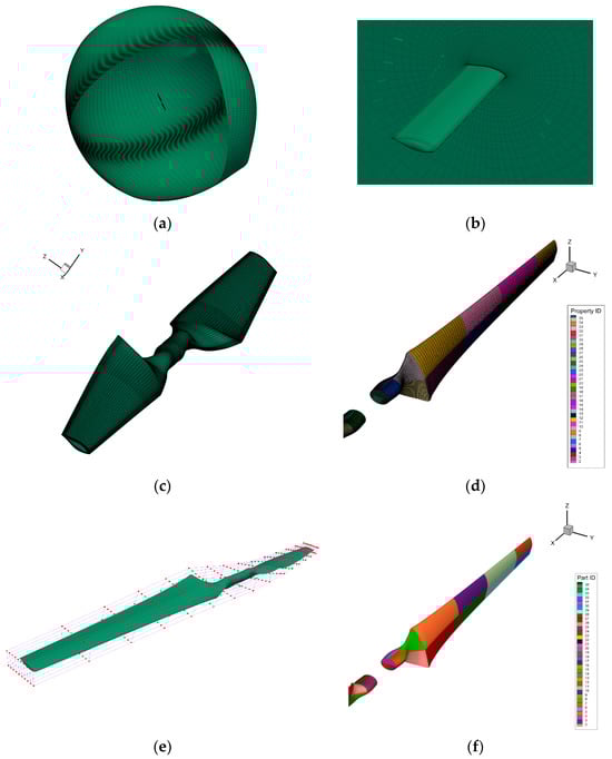
Figure 5.
(a) Spherical volume mesh; (b) hyperbolic expansion layer; (c) aerodynamic surface mesh; (d) structural mesh; (e) FFD points for aerodynamic optimization; (f) structural design variables (in terms of panels with random colors).
4. Mesh Convergence and Validation
Based on the multi-reference frame (MRF), a steady-state method used in computational fluid dynamics (CFD) to describe problems with rotating components, a mesh convergence study was conducted using three levels of mesh: L0, L1, and L2, as shown in Table 2. The wind speed is 7 m/s and the rotor’s rotating speed is 72 pm. In order to maintain a value of y+ close to 1, the growth ratio is set to 1.2 and the initial cell height away from the turbine surface is set to 0.00003 m. y+ is the nondimensional distance from the wall to the first mesh node, and the superscript cross denotes normalization with the axis that used to be the distance.
Table 2.
Mesh convergence by comparing the torque result from simulation against experimental value.
According to Table 2, the torque errors for the three L0-, L1-, and L2-based CFD mesh simulations are 5.35 percent, 10.19 percent, and 13.63 percent, respectively, when compared to the NREL experimental value. However, owing to the high cost of computing, L2 mesh is utilized in our optimization.
As shown in Figure 6, the estimated Cp distribution from the CFD simulation using the L2 mesh at the spans 30%, 47, 63, 80, and 95% is compared with the experimental data from NREL. The experimental result and the CFD findings agree.
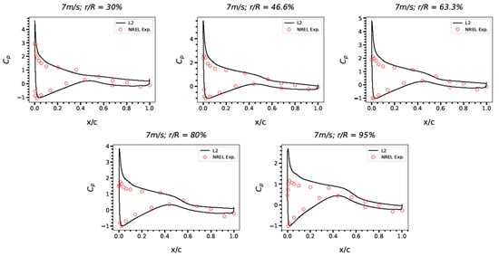
Figure 6.
Comparison of the pressure coefficients (Cp) from level 2 mesh and NREL experimental data.
In Table 3, the computer used is characterized and the computational time is listed.
Table 3.
Computer’s characteristics and computational time.
5. Results and Discussion
The configuration for aerostructural optimization is summarized in Table 4. While the structural optimization seeks to minimize mass, the aerodynamic optimization is more concerned with torque. Figure 5e shows a body-fitted FFD box for the blade. Only the top six layers of FFD points are permitted to shift, creating 240 form variables for the blade as a consequence. This prevents mesh quality issues. Several geometric and physical restrictions, such as a minimal blade volume restriction to prevent the blade volume from falling below three times its baseline volume and thickness restrictions to prevent the blade from becoming too thin, are used to assure practical design. With a maximum nonorthogonality and skewness of 78 degrees and 5.8, respectively, two mesh quality limits are placed on the volume mesh deformation to handle mesh deformation issues. The mesh quality values are calculated using the OpenFOAM checkMesh function, and the constraint derivatives are automatically differentiated using DAFoam. In order to prevent structural failure, an aggregated von Mises stress limitation is applied together with a panel thickness constraint. The stress constraint value, which is an approximate maximal stress value normalized by the material yield stress, is calculated using the Kreisselmeier–Steinhauser function.
Table 4.
Overview of the aerostructural optimization cases.
Figure 7 shows the pressure and stress on the aerodynamic and structural side respectively after the optimization.
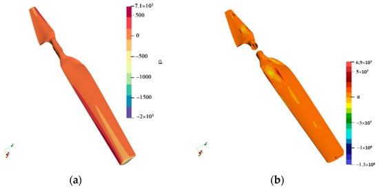
Figure 7.
(a) Pressure on the blade on the aerodynamic side (Pa); (b) stress on the structural side (Pa).
Figure 8a shows that following optimization, the pressure coefficient varies more significantly closer to the tip while being more stable farther away from the root. The cross-section profile of the blade in terms of the three separate sections along the blade is also shown in Figure 8b before and after the optimization. The leading edge and middle portion are improved to provide greater aerodynamic performance.
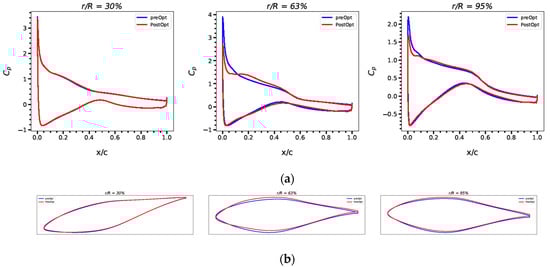
Figure 8.
(a) Cp comparisons before and after the optimization in terms of 30%, 63%, and 95% spanwise section; (b) shape changes in the cross-section profiles accordingly.
According to Figure 9 the torque was increased by around 6.78 percent as the main goal of the aerodynamic portion of the aerostructural optimization. The torque production of the wind turbine blade increased by around 6.78 percent as a result of this optimization procedure. The optimization of the blade’s form is responsible for the increase in torque. By improving this aspect, the airflow around the blade can be better managed, which improves the efficiency with which wind energy is transferred to the turbine blades.
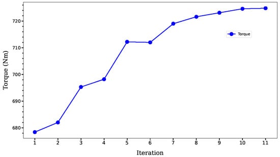
Figure 9.
Torque optimization during aerostructural optimization.
The wind turbine’s total efficiency and power production significantly increased thanks to the 6.78 percent rise in torque output. Since the turbine can produce more electricity with the same quantity of wind, this improved efficiency may result in lower energy prices. The optimization procedure may also result in lower maintenance costs due to decreased component wear and tear brought on by better efficiency.
The term “optimization” in the context of blade design refers to the process of changing different blade design parameters in order to accomplish a certain objective. In this instance, the objective is to reduce the blade’s bulk while preserving its structural integrity. In order to do this, Mphys is used to shift the aerodynamic load on the blade to its structural component. To distribute the weight properly and lessen stress concentrations, the blades’ panel thicknesses must be changed.
The mass of the blade is continuously measured and recorded throughout the optimization process. The findings are shown in Figure 10, which indicates that with each optimization step, the mass of the blade reduces. After the sixth iteration, the rate of decline slows down, indicating that future tweaks would not result in substantial mass reductions. The mass of the blade also decreased by 4.22 percent as a consequence of the optimization process, which has the potential to significantly increase the turbine’s performance and efficiency.
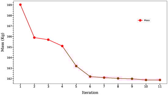
Figure 10.
Mass optimization during aerostructural optimization.
6. Conclusions
This research offered an analysis of a wind turbine blade’s aerostructural optimization. For the aerodynamic portion of the study, DAFoam software (v3.0.3) was used, while TACs was used for the structural portion. The OpenMDAO framework was used to implement the fluid–structure interaction between the CFD and FEM. Torque was the goal for the aerodynamic component, while mass reduction was the goal for the structural component.
The findings of the optimization revealed a 6.78 percent increase in torque and a 4.22 percent decrease in mass. These findings show that the aerostructural optimization strategy can significantly boost the efficiency of wind turbine blades. The weight of the turbine can be made lighter overall by lowering the mass of the blade, which lowers the cost of production and shipping. Additionally, a higher torque can boost the turbine’s energy production, increasing its effectiveness.
The OpenMDAO framework’s integration of DAFoam, TACs, and Mphys made it possible to analyze the wind turbine blade in its entirety. The combination of these software tools made it easier to combine the structural and aerodynamic properties of the blade, allowing for design optimization. The outcomes of the optimization show how crucial it is to take into account both the structural and aerodynamic properties of wind turbine blades when designing them.
In conclusion, this work shows how aerostructural optimization can enhance the performance of wind turbine blades. The optimization’s results show that by reducing the bulk of the blade, there is the possibility for considerable increases in energy output and cost savings. Future research might concentrate on improving the optimization method’s effectiveness and determining whether it can be used with different kinds of wind turbines.
Author Contributions
Y.Z. oversaw the project and provides the fund as well as the equipment; S.B. developed the geometry, CFD analysis, and optimization process and wrote the manuscript. A.B. (Aigerim Baidullayeva) assisted with the mesh generation and manuscript. A.B. (Akerke Baigarina), Y.S. and E.S. participated in the revision and review. Y.Z. and D.W. reviewed and edited the manuscript. All authors have read and agreed to the published version of the manuscript.
Funding
This study is funded by Nazarbayev University through a FDCR grant no. 20122022FD4126.
Data Availability Statement
Data are available upon request to the first author (shaheidula.batai@nu.edu.kz).
Acknowledgments
The authors would like to thank Nazarbayev University for the financial support for this work through a FDCR grant no. 20122022FD4126.
Conflicts of Interest
The authors declare no conflict of interest.
References
- García Maldonado, E. Análisis de las causas de la migración en el contexto del cambio climático según el grupo intergubernamental de expertos sobre el Cambio Climático. Rev. Col. San Luis 2022, 12, 1–32. [Google Scholar] [CrossRef]
- Zhou, Y.; Luckow, P.; Smith, S.J.; Clarke, L. Evaluation of global onshore wind energy potential and generation costs. Environ. Sci. Technol. 2012, 46, 7857–7864. [Google Scholar] [CrossRef] [PubMed]
- Jacobson, M.Z.; Delucchi, M.A. A path to sustainable energy by 2030. Sci. Am. 2009, 301, 58–65. [Google Scholar] [CrossRef] [PubMed]
- Şahin, A.D. Progress and recent trends in wind energy. Prog. Energy Combust. Sci. 2004, 30, 501–543. [Google Scholar] [CrossRef]
- Ackermann, T.; Söder, L. An overview of wind energy-status 2002. Renew. Sustain. Energy Rev. 2002, 6, 67–127. [Google Scholar] [CrossRef]
- Irena, I.-E. IRENA-Wind Power-Technology Brief. 2016. Available online: https://www.irena.org/publications/2016/Mar/Wind-Power (accessed on 10 December 2023).
- Muskulus, M.; Schafhirt, S. Design optimization of wind turbine support structures-a review. J. Ocean Wind Energy 2014, 1, 12–22. [Google Scholar]
- Banos, R.; Manzano-Agugliaro, F.; Montoya, F.; Gil, C.; Alcayde, A.; Gómez, J. Optimization methods applied to renewable and sustainable energy: A review. Renew. Sustain. Energy Rev. 2011, 15, 1753–1766. [Google Scholar] [CrossRef]
- Lei, M.; Shiyan, L.; Chuanwen, J.; Hongling, L.; Yan, Z. A review on the forecasting of wind speed and generated power. Renew. Sustain. Energy Rev. 2009, 13, 915–920. [Google Scholar] [CrossRef]
- Ramirez-Rosado, I.J.; Fernandez-Jimenez, L.A.; Monteiro, C.; Sousa, J.; Bessa, R. Comparison of two new short-term wind-power forecasting systems. Renew. Energy 2009, 34, 1848–1854. [Google Scholar] [CrossRef]
- Costa, A.; Crespo, A.; Navarro, J.; Lizcano, G.; Madsen, H.; Feitosa, E. A review on the young history of the wind power short-term prediction. Renew. Sustain. Energy Rev. 2008, 12, 1725–1744. [Google Scholar] [CrossRef]
- Sfetsos, A. A comparison of various forecasting techniques applied to mean hourly wind speed time series. Renew. Energy 2000, 21, 23–35. [Google Scholar] [CrossRef]
- Zhang, Y.; Wang, J.; Wang, X. Review on probabilistic forecasting of wind power generation. Renew. Sustain. Energy Rev. 2014, 32, 255–270. [Google Scholar] [CrossRef]
- Miller, A.; Chang, B.; Issa, R.; Chen, G. Review of computer-aided numerical simulation in wind energy. Renew. Sustain. Energy Rev. 2013, 25, 122–134. [Google Scholar] [CrossRef]
- Platt, A. Available online: https://github.com/OpenFAST/openfast (accessed on 10 December 2023).
- Bortolotti, P.; Bottasso, C.L.; Croce, A. Combined preliminary–detailed design of wind turbines. Wind Energy Sci. 2016, 1, 71–88. [Google Scholar] [CrossRef]
- Heinz, J.C.; Sørensen, N.N.; Zahle, F. Fluid–structure interaction computations for geometrically resolved rotor simulations using CFD. Wind Energy 2016, 19, 2205–2221. [Google Scholar] [CrossRef]
- Scott, S.; Macquart, T.; Rodriguez, C.; Greaves, P.; McKeever, P.; Weaver, P.; Pirrera, A. Preliminary validation of ATOM: An aero-servo-elastic design tool for next generation wind turbines. J. Phys. Conf. Ser. 2019, 1222, 012012. [Google Scholar] [CrossRef]
- Del Carre, A.; Muñoz-Simón, A.; Goizueta, N.; Palacios, R. SHARPy: A dynamic aeroelastic simulation toolbox for very flexible aircraft and wind turbines. J. Open Source Softw. 2019, 4, 1885. [Google Scholar] [CrossRef]
- Marten, D.; Wendler, J.; Pechlivanoglou, G.; Nayeri, C.N.; Paschereit, C.O. QBLADE: An open source tool for design and simulation of horizontal and vertical axis wind turbines. Int. J. Emerg. Technol. Adv. Eng. 2013, 3, 264–269. [Google Scholar]
- Leimeister, M.; Kolios, A.; Collu, M. Development of a framework for wind turbine design and optimization. Modelling 2021, 2, 105–128. [Google Scholar]
- Madsen, M.H.A.; Zahle, F.; Sørensen, N.N.; Martins, J.R. Multipoint high-fidelity CFD-based aerodynamic shape optimization of a 10 MW wind turbine. Wind Energy Sci. 2019, 4, 163–192. [Google Scholar] [CrossRef]
- Horcas, S.G.; Ramos-García, N.; Li, A.; Pirrung, G.; Barlas, T. Comparison of aerodynamic models for horizontal axis wind turbine blades accounting for curved tip shapes. Wind Energy 2023, 26, 5–22. [Google Scholar] [CrossRef]
- Ramos-García, N.; Sessarego, M.; Horcas, S.G. Aero-hydro-servo-elastic coupling of a multi-body finite-element solver and a multi-fidelity vortex method. Wind Energy 2021, 24, 481–501. [Google Scholar] [CrossRef]
- Lee, K.; Huque, Z.; Kommalapati, R.; Han, S.-E. Fluid-structure interaction analysis of NREL phase VI wind turbine: Aerodynamic force evaluation and structural analysis using FSI analysis. Renew. Energy 2017, 113, 512–531. [Google Scholar] [CrossRef]
- Wainwright, T.R.; Poole, D.J.; Allen, C.B.; Appa, J.; Darbyshire, O. High Fidelity Aero-Structural Simulation of Occluded Wind Turbine Blades. In Proceedings of the AIAA Scitech 2021 Forum, Online, 11–15 January 2021; p. 0950. [Google Scholar]
- Cheng, P.; Huang, Y.; Wan, D. A numerical model for fully coupled aero-hydrodynamic analysis of floating offshore wind turbine. Ocean Eng. 2019, 173, 183–196. [Google Scholar] [CrossRef]
- Gray, J.S.; Hearn, T.A.; Moore, K.T.; Hwang, J.; Martins, J.R.; Ning, A. Automatic evaluation of multidisciplinary derivatives using a graph-based problem formulation in OpenMDAO. In Proceedings of the 15th AIAA/ISSMO Multidisciplinary Analysis and Optimization Conference, Atlanta, GA, USA, 16–20 June 2014; p. 2042. [Google Scholar]
- Ning, A.; Petch, D. Integrated design of downwind land-based wind turbines using analytic gradients. Wind Energy 2016, 19, 2137–2152. [Google Scholar] [CrossRef]
- Ingersoll, B.; Ning, A. Efficient incorporation of fatigue damage constraints in wind turbine blade optimization. Wind Energy 2020, 23, 1063–1076. [Google Scholar] [CrossRef]
- Bortolotti, P.; Dixon, K.; Gaertner, E.; Rotondo, M.; Barter, G. An efficient approach to explore the solution space of a wind turbine rotor design process. J. Phys. Conf. Ser. 2020, 1618, 042016. [Google Scholar] [CrossRef]
- Bottasso, C.L.; Campagnolo, F.; Croce, A. Multi-disciplinary constrained optimization of wind turbines. Multibody Syst. Dyn. 2012, 27, 21–53. [Google Scholar] [CrossRef]
- Hand, M.M.; Simms, D.A.; Fingersh, L.J.; Jager, D.W.; Cotrell, J.R.; Schreck, S.; Larwood, S.M. Unsteady Aerodynamics Experiment Phase VI: Wind Tunnel Test Configurations and Available Data Campaigns; National Renewable Energy Lab.: Golden, CO, USA, 2001. [Google Scholar]
- Batay, S.; Baidullayeva, A.; Zhao, Y.; Wei, D. Aero-Structural Design Optimization of Wind Turbine Blades. Preprints 2023, 2023101072. [Google Scholar] [CrossRef]
- He, P.; Mader, C.A.; Martins, J.R.; Maki, K.J. Dafoam: An open-source adjoint framework for multidisciplinary design optimization with openfoam. AIAA J. 2020, 58, 1304–1319. [Google Scholar] [CrossRef]
- Boopathy, K.; Kennedy, G.J. Parallel finite element framework for rotorcraft multibody dynamics and discrete adjoint sensitivities. AIAA J. 2019, 57, 3159–3172. [Google Scholar] [CrossRef]
- Gray, J.S.; Hwang, J.T.; Martins, J.R.; Moore, K.T.; Naylor, B.A. OpenMDAO: An open-source framework for multidisciplinary design, analysis, and optimization. Struct. Multidiscip. Optim. 2019, 59, 1075–1104. [Google Scholar] [CrossRef]
- Bons, N.P.; Martins, J.R.; Odaguil, F.I.; Cuco, A.P.C. Aerostructural wing optimization of a regional jet considering mission fuel burn. ASME Open J. Eng. 2022, 1, 011046. [Google Scholar] [CrossRef]
- Sgueglia, A.; Schmollgruber, P.; Bartoli, N.; Benard, E.; Morlier, J.; Jasa, J.; Martins, J.R.; Hwang, J.T.; Gray, J.S. Multidisciplinary design optimization framework with coupled derivative computation for hybrid aircraft. J. Aircr. 2020, 57, 715–729. [Google Scholar] [CrossRef]
- Lafage, R.; Defoort, S.; Lefebvre, T. WhatsOpt: A web application for multidisciplinary design analysis and optimization. In Proceedings of the AIAA Aviation 2019 Forum, Dallas, TX, USA, 17–21 June 2019; p. 2990. [Google Scholar]
- Martins, J.R. Aerodynamic design optimization: Challenges; perspectives. Comput. Fluids 2022, 239, 105391. [Google Scholar] [CrossRef]
- Spalart, P.; Allmaras, S. A one-equation turbulence model for aerodynamic flows. In Proceedings of the 30th Aerospace Sciences Meeting and Exhibit, Reno, NV, USA, 6–9 January 1992; p. 439. [Google Scholar]
- Kenway, G.K.; Mader, C.A.; He, P.; Martins, J.R. Effective adjoint approaches for computational fluid dynamics. Prog. Aerosp. Sci. 2019, 110, 100542. [Google Scholar] [CrossRef]
- Balay, S.; Abhyankar, S.; Adams, M.; Brown, J.; Brune, P.; Buschelman, K.; Dalcin, L.; Dener, A.; Eijkhout, V.; Gropp, W.; et al. PETSc Users Manual: Revision 3.10; Office of Scientific and Technical Information (OSTI): Alexandra, VA, USA, 2018. [Google Scholar]
- He, P.; Mader, C.A.; Martins, J.R.; Maki, K.J. An aerodynamic design optimization framework using a discrete adjoint approach with OpenFOAM. Comput. Fluids 2018, 168, 285–303. [Google Scholar] [CrossRef]
- Martins, J.R.; Hwang, J.T. Review and unification of methods for computing derivatives of multidisciplinary computational models. AIAA J. 2013, 51, 2582–2599. [Google Scholar] [CrossRef]
- Batay, S.; Kamalov, B.; Zhangaskanov, D.; Zhao, Y.; Wei, D.; Zhou, T.; Su, X. Adjoint-Based High Fidelity Concurrent Aerodynamic Design Optimization of Wind Turbine. Wind Energy Sci. Discuss. 2022, 8, 85. [Google Scholar] [CrossRef]
- Secco, N.R.; Kenway, G.K.; He, P.; Mader, C.; Martins, J.R. Efficient mesh generation and deformation for aerodynamic shape optimization. AIAA J. 2021, 59, 1151–1168. [Google Scholar] [CrossRef]
Disclaimer/Publisher’s Note: The statements, opinions and data contained in all publications are solely those of the individual author(s) and contributor(s) and not of MDPI and/or the editor(s). MDPI and/or the editor(s) disclaim responsibility for any injury to people or property resulting from any ideas, methods, instructions or products referred to in the content. |
© 2023 by the authors. Licensee MDPI, Basel, Switzerland. This article is an open access article distributed under the terms and conditions of the Creative Commons Attribution (CC BY) license (https://creativecommons.org/licenses/by/4.0/).